A Markov Switching Model of the Merit Order to
Compare British and German Price Formation
∗
Georg Zachmann
†15.03.2006
Preliminary Version. Please do not quote.
Abstract
The objective of this paper is to develop a model to determine the ef-ficient functioning of wholesale electricity markets. For that purpose, we model wholesale electricity prices depending on the prices of fuels (e.g., coal and natural gas) and of CO2 emission allowances using a Markov
Switching Regression. We apply the model to wholesale electricity prices in the UK and in Germany. While British electricity prices are quite well explained by short-run cost factors, we find a decoupling between elec-tricity prices and fuel costs in Germany. This may be evidence that the German electricity generation sector does not work competitively.
Keywords: Electricity Prices, Markov Switching Models
JEL classification: L94, C22, D43
∗The author would like to thank Derek Bunn, Christian von Hirschhausen and Franziska
Holz for their many helpful comments and discussions regarding this work. All remaining errors are the author’s sole responsibility.
1
Introduction
Electricity markets differ from other commodity markets in various respects. Demand for electricity is inelastic in the short term, storing it is impossible, parts of the value chain exhibit characteristics of natural monopolies and reli-able electricity supply has high macroeconomic importance. In the potentially competitive wholesale sector, remaining vertical and horizontal integration as well as the widespread existence of national incumbents are often providing significant market power. Whether this market power is actually exercised in one market or the other is an open issue. To drive prices in the desired di-rection, players could basically apply three strategies: withholding capacity, over-bidding their marginal cost or under-bidding their marginal cost. Whereas capacity withholding and over-bidding will raise the wholesale price and thus potentially increase profits for the generators, under-bidding might be ”appro-priate” to create excess revenues for the vertically integrated electricity supply companies [e.g., K¨uhn Machado (2004)]. To detect such strategic behavior it would be desirable to compare the cost curves for each market participant to its actual bids. But the true cost functions are private information. In addition, individual or even aggregated bid curves are unavailable for scientific inquiries in many markets (e.g., the EEX in Germany publishes neither individual nor aggregated bid curves).
Nevertheless to enquire whether wholesale electricity markets determine jus-tifiable prices, various indirect approaches have been proposed. Analyzing bid-ding data of electricity auctions, Hortacsu and Puller (2004), Wolfram (1998) and Sweeting (2004) are able to provide evidence for strategic bidding. Sweeting (2004) finds that bidding behavior became consistent with tacit collusion after 1995-96 in the English and Welch wholesale market. Studying the bidding be-havior of National Power and PowerGen in the English and Welch market, Wol-fram (1998) provides evidence for strategic bidding. And Hortacsu and Puller (2005) compares firm-level marginal cost and bids in the Texas electricity spot market, finding that smaller firms especially were bidding strategically. Wolfram (1999) and M¨usgens (2004) also estimate marginal cost, but compare those to the actual prices (not the bids). Wolfram (1999) estimates the price-cost mar-gin in the British market, finding that the strictly positive marmar-gins were lower than implied by theoretical models, which she explained by regulation, threat of entry and supplier-customer relations. Finally, M¨usgens (2004) simulates the marginal cost of the German electricity system and compares those to the ac-tual prices. He finds that prices decoupled from short-run marginal cost in the years 2000 to 2003. His simulation of electricity generation cost is based on an extensive model of the German market using a large-scale power plant database. Essentially, the model optimizes the German system with respect to the actual demand.1 The marginal costs of the last required generator set the marginal
cost of the entire system. The accurate representation of the market allows prices to be forecasted, to simulate the effects of institutional and other changes
1M¨usgens (2004) model set-up is quite sophisticated, taking into account, for example, cross-border electricity trade and the dynamic optimization decision of hydro power plants.
and to analyze deviations from forecasts. On the other hand the calibration of such large models encompasses a number of uncertainties and validating the results turns out to be difficult.
In this paper we propose a different approach. Instead of calculating the absolute deviation of the electricity price from the respective generation cost, our goal is to obtain a relative indicator for the cost-reflectiveness of national electricity prices. Therefore, we first set up a stylized model of the marginal electricity generation cost. In asecond step, the model is estimated over time assuming that prices equal marginal cost. Finally, the coefficients and the resid-uals of the estimation are compared across countries to assess where and when prices are best explained by their fundamentals. Thus, the model should also be able to identify deviations from competitive price setting.
The paper is structured in the following way: the next section presents the model. Section 3 introduces some stylized facts on the countries to which we apply the model: the UK and Germany. Section 4 presents the results and an interpretation. Finally, the policy implications are outlined in the conclusion.
2
Model
The cost of a power plant is mainly composed of capital, labor and fuel cost.2 In the short run (less than six month), the fuel component is the most important factor for two reasons: First, in this time horizon a thermal power plant can only adjust its cost by reducing or increasing the fuel input. And second, fuel prices change much more frequently and more strongly than capital or labor cost. Thus, in the absence of structural changes that alter the long- and medium-term cost of power plants, the cost of a power plant is correlated dominantly with the price of the fuel that it burns and the related emission certificates. If bid prices were set according to cost, the electricity price should be correlated with the price of the fuel and the cost of emissions of the marginal power plant at any point in time. To deduce analytically which of the generators is the marginal unit, sizeable models have been applied in the past. By accurately reproducing the entire energy sector, they are able to identify the last required unit at every point in time. This requires detailed information of the cost structure of every single power plant as well as on the demand. These heavy information requirements make these models impractical for international comparison, since consistent databases do not exist so far.
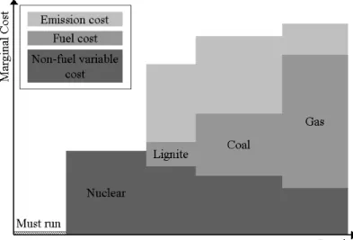
Hence we will present a new approach of representing the electricity price formation mechanism, using a stylized model of electricity markets. In contrast to other markets, electricity markets are characterized by a set of different pro-duction technologies with very different marginal cost. The non-storability of electricity allows that large nuclear power plants with low variable costs, coal-fired generators with medium variable costs, and small gas turbines with high variable costs can coexist. Because the differences of marginal costs of power plants of the same technology are small compared to the cost difference between
Figure 1: Stylized example of the stepwise marginal cost function
dissimilar technologies, the marginal cost curve of the entire electricity system can be approximated by a stepwise function (see Figure 1).3
Based on this assumption, one can model the electricity price at timetas the marginal cost of the last required technology to meet the demand. As outlined above, in the short run the cost of a power plant should be highly correlated with its fuel and emission cost. Since the fuel efficiency of technologies changes rather slowly, fuel and emission costs are predominantly determined by the respective prices. Thus, a time series model that endogenously infers the cost structures of each class of power plants and that deduces which class is marginal at each point in time can be set up using fuel, emission and electricity prices as only input. Generally the model consists of two procedures: a routine that decides which class of power plants sets the price (i.e., is marginal) and a mechanism that reproduces the electricity price formation for each class.
For each technology (S = 1, ..., m) we assume the marginal costs at time t
to be the sum of a weighted linear combination of thek explanatory variables (βSt×Xt) and a stochastic component (t,St). The set of explanatory variables
stored in the columns of the matrixX might contain for example a constant, a time trend, different dummy variables as well as gas, oil, coal and emission certificate prices.
3Typical non-dispatchable must-run generation are wind, run-of-river hydro and combined heat and power plants (in winter).
Thus, depending on the chosen explanatory variables and the technologies the model can be written as:
pel,t= β1×Xt+t,1 ifSt= 1 β2×Xt+t,2 ifSt= 2 .. . βm×Xt+t,m ifSt=m (1)
When the process that determines the marginal technology at time tis as-sumed to be Markovian4, (1) can be estimated using a Markov Switching
Re-gression. To do this, the model has to be converted into state space form with the states (or regimes) of the model representing the different technolo-gies. To make the model computable, the Markovian Process is specified as
P(St=i|St=j) =pi,j i.e. with time invariant exogenous switching probabili-ties.5 Thus the model is fully described by
pel,t=βSt×Xt+t,St, ∀St= 1..m (2)
P=P(St=i|St−1=j) =pi,j, ∀i, j≤m (3)
where Xt is the (k×t) matrix of explanatory variables, βSt is the state
de-pendent (1×n) row vector (βSt,1, βSt,2, . . . , βSt,n), andP is a (m×m) matrix
containing the probability to switch from state i to state j. Note that in a stylized world where only three types of power plants (i.e. gas, coal, oil) exist, for each technology only the constant, the coefficient for the price of the used fuel and the coefficient for the price of emission certificates should be nonzero.
The interpretation of these coefficients would then be straightforward. The constant would represent the fixed cost of this type of power plants. The fuel coefficient for the used fuel would be the heat rate of this type of power plants (when electricity price and fuel price are both measured in the same unit i.e. Euro/MWh). And the coefficient for the emission certificate prices represents the amount of emissions per unit of electricity.6 An issue which we do not
adress in this context is the endogeneity problem. That is, we ignore that gas and emission allowance prices also depend on electricity prices. This has been kept in mind for the interpretation of the results.
In our non-linear model it is difficult to deduce theoretically the distribution of the parameters conditioned on the data. This challenge can be circumvented by using the Gibbs sampling technique.7 The idea is to repeatedly draw each parameter conditioning on the data and all other parameters. This procedure
4A Markovian process is characterized by the fact, that each observation only depends on the last period.
5It would be useful to include demand and weather conditions into the switching proba-bilities, but this has not been possible in this paper.
6The units match accordingly:
Eur/MWhel=Eur/MWhel+MWhel/MWhth×Eur/MWhth+tCO2/MWhel×Eur/tCO2 7See Krolzig (1997).
is iterated a large number of times, always conditioning on the latest draws of the other parameters.
To estimate (2) and (3) via Gibbs sampling, the density function of the model can be separated as:
g(ST, βSt,ΣSt, P|yt, Xt) =g(βSt,ΣSt|yt, Xt, St)g(P|ST)g(ST|yT, XT) (4)
Therefore one proceeds in four steps:
1. Generate g(ST|yt, Xt, βSt,ΣSt, P) using the Hamilton filter that deduces
g(St|St+1, yt, Xt) from theg(St|yt, Xt).
2. Draw the beta-distributed switching probabilitiesP givenSt. 3. Draw theβSt givenyt,Xt,Stand ΣtSt.
4. Draw the ΣSt givenβSt,yt,Xt andSt.
A detailed description of the four steps can be found in Schweri (2004) who also provides the corresponding Matlab code. Since valuable prior knowledge on the distribution of various parameters was available, the model was estimated in the Bayesian framework that allows this information to be included. In each of the steps the posterior distribution p(θ|y) is thus given by the likelihood functionL(θ|y) times the prior distributiong(θ):
p(θ|y) =g(θ)×L(θ|y) (5) Thus, to implement the estimation, the informal prior knowledge on the characteristics of the parameters has to be transformed into formalized prior distributions. The explained and explanatory variables have to be selected, and starting values to initialize the described algorithm have to be chosen. After briefly introducing the electricity sectors in the UK and Germany, two different models and the associated results will be presented in Section 4.
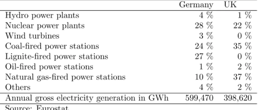
Table 1: Gross electricity generation (2003) Germany UK
Hydro power plants 4 % 1 %
Nuclear power plants 28 % 22 %
Wind turbines 3 % 0 %
Coal-fired power stations 24 % 35 % Lignite-fired power stations 27 % 0 % Oil-fired power stations 1 % 2 % Natural gas-fired power stations 10 % 37 %
Others 4 % 2 %
Annual gross electricity generation in GWh 599,470 398,620 Source: Eurostat
3
Data
We want to apply the model to assess the functioning of two national wholesale electricity markets, the UK and Germany. The UK market is generally consid-ered to be competitive, whereas substantive concerns have been raised against the proper functioning of the Germany market. Both wholesale markets are particularly suited to be analyzed using the model described above. First, nei-ther of these markets is endowed with significant hydro power capacity This is an advantage since the model is unable to reproduce the dynamic opportunity cost assessment required for analyzing the marginal cost of a hydro power plant.
Second, both countries feature liquid wholesale markets that provide reference prices. Andthird, it is widely agreed upon that liberalization in the electricity sector is more advanced in the UK than it is in Germany.8 Thus we can compare the model results to this prior knowledge.
In terms of size, the German and the British system are approximately com-parable (see Table 1). Conventional thermal power plants account for more than 60% of the fuel mix in both countries (62% in Germany and 74% in the UK). One obvious difference between both systems is that the UK does not use lignite for which it compensates by an increased share of natural gas. Market structure and design in both countries differ markedly. Whereas the UK has two decades of experience with market opening and regulation, Germany has adressed sec-tor reforms only in the first part of this decade, and a regulasec-tor was set up in mid-2005. The four privately owned transmission system operators in Germany have significant stakes in generation (together 80% of total capacity) and distribution. The integration of the two major German players E.on and RWE -with their natural gas affiliates further increases their dominating position. In the UK the situation is more balanced. The transmission system operator is state owned and regulation is effective. The nine biggest generation companies together own only 68% of the capacities. Although these are integrated with electricity and gas suppliers, none of them has a position comparable to the ”big
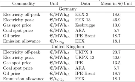
Table 2: Summary of the data sample
Commodity Unit Data Mean ine/Unit Germany
Electricity off-peak e/MWhel EEX 3 18.6 Electricity peak e/MWhel EEX 13 46.9 Gas spot price e/MWhth Zeebrugge 13.0 Coal spot price e/MWhth ARA 5.7 Oil price e/MWhth IPE Brent 18.7 Emission allowance e/tCO2 EEX 18.1
United Kingdom
Electricity off-peak e/MWhel UKPX 3 23.7 Electricity peak e/MWhel UKPX 13 40.0 Gas spot price e/MWhth IPE 13.5 Coal spot price e/MWhth ARA 5.7 Oil price e/MWhth IPE Brent 18.7 Emmission allowance e/tCO2 EEX 18.1
four” in Germany.
To compare the relation of cost and prices in both markets, data on the rele-vant national electricity, fuel and emission prices are required. Since the model (described in the next section) is only meaningful in the short and medium run, daily price notations are used for all commodities. Because no daily German gas, oil and coal prices are available for the entire sample, the respective values of the relevant markets in Belgium (Zeebrugge)9, the UK (IPE Brent) and the Netherlands (ARA) were selected.10 Despite the Zeebrugge gas prices, all data
were converted to Euro by and obtained from Datastream. The sample contains data from January 2002 to December 2005. Because gas and coal prices are only available for working days, week-ends and holidays are omitted from the sam-ple.11 The fuel prices are converted intoe/MWh
th to ease the interpretation. The respective data sources for the four commodities for Germany and the UK are summarized in Table 2.
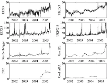
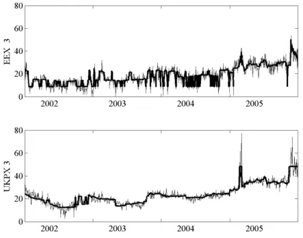
Figure 2 depicts the series of spot prices. Peak and off-peak electricity prices approximately doubled between 2002 and 2005. Gas prices also doubled, whereas coal prices reached their initial level at the end of 2005 .12 Emission
allowance prices increased from around 10 ein early 2005 to around 20 eat the end of this year.
Electricity, fuel and emission allowance prices are mutually interdependent
9Bunde(D) and TTF(NL) do not provide data for the entire sample period
10EEX3 and EEX13 address the third and thirteens hour EEX price whereas UKPX3 and UKPX13 address the seventh (3am-3.30am) and the twenty-seventh (1pm-1.30pm) half hourly UKPX price.
11This has the positive side effect of reducing seasonalities significantly.
12Datastream derives the daily coal price notations by converting the monthly coal prices in dollar into euro using the daily exchange rate. Thus, the increasing dollar-euro exchange rate limited the effect of rising coal prices for European coal consumers.
Figure 2: Development of the spot price series 2002-2005
Table 3: Results of an OLS for the electricity spot prices 2002-2005 Const Trend Gas Coal CO2 R2 ˆσ2
EEX3 6.11** 0.005** 0.37** 0.64** 0.37** 0.61 28.5 EEX13 43.8** 0.026** 1.12** -4.58** 0.34 * 0.36 343.3 UKPX3 5.63** -0.008** 0.53** 2.07** 0.66** 0.79 17.6 UKPX13 19.73** 0.013 * 1.09** -0.84 0.79** 0.40 396.0
via substitution and production relations and they are partly influenced by similar external factors (e.g., weather). The common upward trend, as well as shared spikes, indicates that these relations translate into statistical links. An ordinary least square (OLS) estimation suggests that electricity prices are influenced by gas, coal and emission allowance prices to a different degree.13 The
results depicted in Table 3 indicate that electricity prices in off-peak depend more significantly on the coal price whereas those in peak are more strongly influenced by the gas price. Due to the higher volatility in the peak prices, the ˆσ2
is significantly higher in peak than in off-peak periods. Thus the ordinary least square model reveals that the relation between electricity prices and fuel as well as emission prices is not stable throughout the day. This leads to questioning the assumption of a stable relationship in the single hour series as it is implied by the presented OLS. We therefore have to cope with the instable links between fuel and emission prices, which is done by implementing the model in the next section.
13The OLS is used here to show that the prices interact significantly and that interaction varies with the daytime. The endogeneity problem is ignored in this context.
4
Results
4.1
Estimation Results
For setting up the test we proceeded in three steps. First, we choose the gen-eral model, i.e., the number of states, the sample period, and the explanatory variables. Second, we decide on the distribution of the initial values and the pri-ors. This has been a rather delicate task since in some models no less than 132 parameters had to be feed in.14 Andthird, the estimation parameters: number of runs, number of initial runs discarded, identification restrictions applied and share of saved runs have to be set.
We estimate (2) and (3) for the off-peak and peak period for the German (EEX) and the British (UKPX) market. For each market, we select one hour of off-peak (3h in the morning) and one hour of peak (13h). All four cases (EEX3, EEX13, UKPX3 and UKPX13) are processed twice: once using a purely data-driven approach (noninformative priors), and once including prior information (informative priors). For the data-driven approach a three-state model15 in
which spot electricity prices are explained by spot gas prices, spot coal prices and the respective emission allowance price is applied. Oil prices and a trend are omitted after initial estimations suggested that they are not significant for any state. Variance and allβcoefficients are selected to be state dependent.16
Start-ing values and prior distribution are chosen as to impose almost no restrictions on the estimations. The prior means for allβ coefficients is adjusted to unity and high prior variance is set.17 Solely with respect to the switching matrix some persistency was predefined to capture the effect that switching from one marginal technology to another only occurs when demand or supply conditions change significantly.18 The results of the three state model with non-informative priors are summarized in Table 4.19
The results confirm the expected superiority of this approach compared to
14In a three state model with three explanatory variables plus a constant we have to prede-fine 24 parameters setting the prior distribution of the coefficients, 18 parameters setting the prior distribution of the switching probabilities and 24 parameters setting the prior distribu-tion of the covariance matrix. In addidistribu-tion to these 66 prior parameters, another 66 starting values have to be selected.
15Numerous estimations suggested that the peak as well as the off-peak data are best cap-tured by three-state models. Two-state models did not reproduce the data equally well and four-state models mainly contained redundant regimes, i.e., the distributions of the parameters of two states were highly interfering.
16Note, that state dependent variance is straightforward since high electricity price regimes are characterized by higher variance.
17Generally, we adjusted the starting values to the value of the respective prior. Solely the
βcoefficients for the constant have been chosen to be different from one, because identification required each state to have different initial values. The identification restriction applied in all models wasβ0
const,St=1< β 0
const,St=2< β 0
const,St=3. The variance of the coefficients has
been set to 100 and the model variance was set to 6.7.
18The probability to remain in the current state was set to 0.67 whereas the probability to switch to each other state was adjusted to 0.16. Giving the prior a modest variance of approximately 0.1, this implies that the beta-distribution of thepij - values is set tou1= 2 andu2= 1 on the main diagonal andu1= 1 andu2= 6 beyond the main diagonal.
Table 4: Results of the Switching Regression with noninformative priors State βˆconst βˆcoal βˆgas βˆCO2 Mean ˆσ
2 Freq 1 2.13 0.99 0.34 0.56 15.8 22.2 443 EEX3 2 6.97 1.15 0.25 1.40 17.1 7.2 297 R2=0.81 3 13.39 0.23 0.57 0.30 24.6 11.0 270 1 -7.16 15.63 0.71 -0.18 75.8 1550.1 129 EEX13 2 13.09 1.67 0.95 0.71 38.3 28.3 514 R2=0.58 3 24.26 1.04 1.19 0.72 48.6 38.6 367 1 -1.62 2.97 0.49 0.42 25.5 10.4 451 UKPX3 2 13.82 0.45 0.28 1.97 20.2 3.9 283 R2=0.92 3 21.81 -0.30 0.30 4.33 24.2 4.8 276 1 12.46 2.36 0.19 0.79 29.5 9.9 619 UKPX13 2 25.22 0.60 0.77 0.73 45.7 54.0 319 R2=0.73 3 55.31 5.32 1.07 -0.43 104.6 2224.7 72
standard OLS.First, the goodness of fit of the switching regression is signifi-cantly better. Second, regimes are substantial and feature quite stable coeffi-cients. This can be seen by fact that the model was able to clearly distinguish between the three regimes.20 Andthird, mostβ values can be interpreted in a meaningful way. In the off-peak scenarios the coefficients in EEX3-1 as well as UKPX3-2 and UKPX3-3 can be interpreted as a situation where baseload pro-ducers with low marginal cost (i.e. lignite, nuclear or wind) were the marginal units, leading to low electricity prices and a low impact of coal and natural gas prices.21 In the EEX3-2 and the UKPX3-1 the off-peak prices are mainly
explained by coal and emission allowance prices which indicate that coal power plants are the marginal producers. This situation occurs less often than the baseload producer state. For Germany, a state with high prices, a significant impact of gas prices occurs (EEX3-3) which can be interpreted as the peri-ods when gas-fired power plants were marginal. Coal is not significant and allowances are less significant in this state. Note that the described states only considered the third hour of the day.
In peak periods, electricity prices behave very differently: prices and variance are higher, price spikes occur and the merit order is known to switch more frequently. Consequently the goodness of fit of the model decreases significantly, even though the three-state model allows us to capture some main features of the peak period price formation mechanism. Essentially a ”coal”, a ”gas” and a ”spike” state can be identified for both countries. In the ”coal” state (EEX13-2 and UKPX13-1) prices are lowest and the coefficients for coal are bigger than those for gas, and emission prices are significant. These states occur for more than half of the time. The ”gas” state (EEX13-3 and
UKPX13-20Note that also the error bands of the coefficients (not reported here) were quite tight. 21Note that it is more likely that the remaining impact of fuel prices on the first regime is due to non-marginal cost-based pricing and stochastic factors than to the feedback effects of balancing markets.
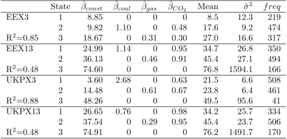
Table 5: Results of the Switching Regression with informative priors State βˆconst βˆcoal βˆgas βˆCO2 Mean ˆσ
2 f req EEX3 1 8.85 0 0 0 8.5 12.3 219 2 9.82 1.10 0 0.48 17.6 9.2 474 R2=0.85 3 18.67 0 0.31 0.30 27.0 16.6 317 EEX13 1 24.99 1.14 0 0.95 34.7 26.8 350 2 36.13 0 0.46 0.91 45.4 27.1 494 R2=0.48 3 74.60 0 0 0 76.8 1594.1 166 UKPX3 1 3.60 2.68 0 0.63 21.5 6.6 508 2 14.48 0 0.61 0.67 23.8 6.4 461 R2=0.88 3 48.26 0 0 0 49.5 95.6 41 UKPX13 1 26.65 0.76 0 0.98 34.2 25.7 334 2 37.54 0 0.29 0.95 45.4 23.7 506 R2=0.48 3 74.91 0 0 0 76.2 1491.7 170
2) features higher prices than the ”coal” state, and its coefficients for gas are higher than those for coal. Finally the ”spike” state (EEX13-1 and UKPX13-3) is characterized by very high prices, extreme volatility, meaningless coefficients and limited occurrence.
Table 5 presents the results of the estimation using informative priors. In each state one or more coefficient have been restricted to zero.22 In the first state (”the coal state”), the gas price coefficient has been set to zero. In the second state (”gas state”) the coal coefficient has been set to zero. And in the no-fuel state (either ”baseload” or ”spike” state) all coefficients apart of the constant have been set to zero.23 This set-up allows one to inquire whether
a pure fuel model, i.e., the perfect case with only these two fuels, is working reasonably well. As expected, the goodness of fit in the restricted version is below that in the unrestricted model. However, the model produces meaningful results. The ”coal state” features usually the highest impact of CO2 prices and
has the lowest electricity prices. The ”gas state” turns out to be influenced by CO2 prices, too. And the third state is in all cases a high price regime (”spike
state”) with a limited number of occurrences.
In Figure 3 the marginal state for every point in time (as estimated in the model with informative priors) is depicted. Some interesting patterns are to be noted: First, the occurrence of the ”baseload” state in the German off-peak series diminished over time whereas the ”gas state” gained importance. This
22Forcing coefficients to be zero was done by setting the mean of its prior distribution to zero and giving this prior a very low variance (here 0.01).
23Due to the identification restriction (see FN 11) the sorting of the no-fuel state has been crucial. Setting it as the first state implied it to have the lowest constant of all states and thus resulted in a ”baseload state”, whereas defining it to be the third state implied that it is a no-fuel-based high-price state. To let the data speak, we estimated both possibilities for all four data sets. It turned out that only the EEX3 is best represented using a ”baseload” state. Given the higher share of wind, nuclear and lignite in Germany, this low price state has a straightforward interpretation.
Figure 3: Development of the marginal state in the model with informative priors
can be either explained by a reduction of cheap production capacities or an increased demand, shifting the equilibrium point towards the higher price fuel.
Second, English off-peak electricity prices tend to be closer related to coal prices in summer and gas prices in winter. However the highest prices at the end of 2005 are only explained by the non-fuel price based ”spike state”. Third, for the German peak series, the influence of coal diminished and gas prices became the driving factor for longer-lasting periods. These were interrupted by randomly occurring price spikes. Andfourth, the English peak series is characterized by frequent switches between coal and gas dependent states. Whereas coal had been prevalent until 2003, thereafter the gas state became more widespread. Again, price spikes occurred at a random frequency.
4.2
Analysis of the Residuals
After having provided evidence that the estimation results are in line with the presented assumptions on the electricity price formation mechanism, we can now make use of this model. We will test two hypotheses: First, it is tested whether the pricing in the UK is more fuel price driven than in Germany. And the second hypothesis to be considered is that short-run marginal cost decoupled from German electricity prices over time. To carry out the tests we use the model with informative priors because the implied restrictions assure more robust results and the model has the desired fundamental interpretation.
The first test is carried out by comparing the error terms of the models using a Kruskal-Wallis test for the hypothesis that the series of the absolute values
Figure 4: Boxplot of the residuals for the 3rd (off-peak) and 13th (peak) hour
of the error terms have the same mean for the German and the British market. For both the peak and the off-peak series, the null hypothesis had to be rejected on any confidence interval.24 It turned out that the mean of the absolute errors
was significantly higher for the model of the German market. This evidence is graphically represented by the boxplots in Figure 4. The better performance of the proposed model for the UK might be explained by three features: First, electricity generation in the UK relies more on the two modelled fuels (34% of gas and coal in the German electricity production vs. 72% in the UK).Second, the feedback effects of the British electricity price on the British gas price are stronger than the respective effects of the EEX prices on the Zeebrugge prices. And third, the British market is more competitive leading to more short-run cost dependent electricity prices.25
To analyze how the ability of the model to explain wholesale electricity prices developed over time, again the respective residuals are analyzed. As depicted in Figure 5 the residuals of the German peak series show a clear upward trend.26
This indicates that the electricity price formation mechanism is distancing from
24For the off-peak residuals the Chi-sq has been 25.0 which leads to a prob value of 5.8e−7. For the peak residual the Chi-sq has been 36.0 leading to a prob value of 2.0e−9. Thus the hypothesis of a common mean has to be rejected on the 99.99% significance level
25Note that the higher pricing efficiency might be due to the closer gate closure in the UK (1h ahead) compared to Germany (12am of the day before).
26A more precise statement is not possible to date, since the depicted t-probabilities are just indicative values because usual t-tests do not apply since the series are not normally distributed. For instance, bootstraping was too computationally extensive, since single runs of the regime-switching model (with 10,000 Gibbs draws) alone took around 30 minutes.
Figure 5: Actual minus estimated electricity price series and trend
fuel-cost foundation. This extends similar findings of M¨usgens (2004)27 to the
period from 2002 to 2005. This development can be attributed to two develop-ments: First, it has been argued that in the sample period electricity pricing switched from over-capacity driven short-run marginal cost (SRMC) pricing af-ter the liberalization to a less fuel cost dependent long-run marginal cost pricing. This switching has been attributed to the reduction of excess capacities in the process of liberalization. A second explanation might be that increasing con-centration in the wholesale sector eased the exercise of market power to raise prices.
27M¨usgens (2004) model indicated that prices before September 2001 were significantly closer to cost than prices from September 2001 to June 2003.
5
Conclusion
The paper compares the wholesale price formation mechanism in the UK and Germany. Applying a Markov switching regression we provide evidence that the electricity wholesale prices in the UK are more closely related to the prices of coal, gas and emission allowances than their German counterparts. These differences in the German and British price formation mechanism shed light on the insufficient integration of these markets. In addition it is shown that the frequency at which high-price fuels became marginal increased in both countries. Given that demand did not increase significantly in the sample period, this can be interpreted as a leftward shift of the supply function, indicating a reduction of available cheap production capacities. Furthermore we provide evidence, that German peak prices increasingly decoupled from their fuel cost fundamentals in the years 2002 to 2005. These findings are in line with conjectures that the exercise of market power became more important for explaining German electricity wholesale prices.
References
[1] Arciniegas, I., Barrett, C., Marathe, A., 2003. Assessing the efficiency of US electricity markets. Utilities Policy 11(2), 75-86.
[2] Borenstein, S., Bushnell, J.B., Wolak., F.A., 2002. Measuring Market Inefficiencies in California’s Restructured Wholesale Electricity Market. American Economic Review 92(5), 1376-405.
[3] Bunn, D.W. (Ed.), 2004. Modelling Prices in Competitive Electricity Markets. John Wiley & Sons, Chichester.
[4] EC, 2005. Report from the Commission on the Implementation of the Gas and Electricity Internal Market (4th Benchmarking Report). Commission Staff Working Document, Brussels.
[5] Fama, E.F., 1970. Efficient Capital Markets: A Review of Theory and Empirical Work. Journal of Finance 25, 383-417.
[6] Hortacsu, A., Puller, S. L., 2005. Testing Models of Strategic Bidding in Auctions: A Case Study of the Texas Electricity Spot Market. NBER Working Paper 11123.
[7] Huisman, R., Mahieu, R., 2003. Regime jumps in electricity prices. Energy Economics 25, 425-434.
[8] Knittel, C.R., Roberts, M.R., 2004. An Empirical Examination of Restruc-tured Electricity Prices. Duke University, University of California.
[9] Krolzig, H.-M., 1997. Markov-Switching Vector Autoregressions. Modelling, Statistical Inference and Application to Business Cycle Analysis. Lecture Notes in Economics and Mathamatical Systems, Vol. 454. Springer, Berlin.
[10] K¨uhn, K.-U., Machado, M., 2004. Bilateral Market Power and Vertical Integration in the Spanish Electricity Spot Market. CEPR Discussion Papers 4590.
[11] Lucia, J.J., Schwartz, E.S., 2001. Electricity Prices and Power Derivatives: Evidence for the Nordic Power Exchange. Review of Derivates Research
5(1), 5-50.
[12] M¨usgens, F., 2004. Market Power in the German Wholesale Electricity Market. EWI Working Paper 04/03.
[13] OXERA, 2003. Energy Market Competition in the EU and G7: The Relative Extent of Energy Market Competition in the EU and G7. Report on Behalf of the UK Department of Trade and Industry, London, Oxford.
[14] Schweri, U., 2004. Regimewechsel und Zustandsraummodelle. Diploma Thesis at Chair of Prof. H. Garbers (University Zurich).
[15] Stoft, S., 2002, Power System Economics: Designing Markets for Electric-ity. John Wiley & Sons, New York.
[16] Sweeting, A. 2004. Market Power in the England and Wales Wholesale Electricity Market: 1995-2000. Working Paper, Northwestern University.
[17] Vehvil¨ainen I., Pyykk¨onen, T., 2005. Stochastic factor model for electricity spot price - the case of the Nordic market. Energy Economics 27, 351- 367.
[18] Wolfram, C. D., 1998. Strategic Bidding in a Multiunit Auction: An Empirical Analysis of Bids to Supply Electricity in England and Wales. RAND Journal of Economics 29(4), 703-725.
[19] Wolfram, C. D., 1999. Measuring Duopoly Power in the British Electricity Spot Market. American Economic Review 89(4), 805-826.