Original Citation:
Optimal transport over a linear dynamical system
Institute of Electrical and Electronics Engineers Inc.
Publisher:
Published version:
DOI:
Terms of use:
Open Access
(Article begins on next page)
This article is made available under terms and conditions applicable to Open Access Guidelines, as described at
http://www.unipd.it/download/file/fid/55401 (Italian only)
Availability:
This version is available at: 11577/3256169 since: 2018-02-12T20:31:28Z
10.1109/TAC.2016.2602103
Università degli Studi di Padova
Optimal transport over a linear dynamical system
Yongxin Chen, Tryphon T. Georgiou and Michele Pavon
Abstract—We consider the problem of steering an initial probability density for the state vector of a linear system to a final one, in finite time, using minimum energy control. In the case where the dynamics correspond to an integrator (x˙(t) = u(t)) this amounts to a Monge-Kantorovich Optimal Mass Transport (OMT) problem. In general, we show that the problem can again be reduced to solving an OMT problem and that it has a unique solution. In parallel, we study the optimal steering of the state-density of a linear stochastic system with white noise disturbance; this is known to correspond to aSchr¨odinger bridge. As the white noise intensity tends to zero, the flow of densities converges to that of the deterministic dynamics and can serve as a way to compute the solution of its deterministic counterpart. The solution can be expressed in closed-form for Gaussian initial and final state densities in both cases.
Keywords: Optimal mass transport, Schr¨odinger bridges, stochastic linear systems, optimal control.
I. INTRODUCTION
We are interested in stochastic control problems to steer the probability density of the state vector of a linear system between an initial and a final distribution for two cases, i) with and ii) without stochastic disturbance. That is, we consider the linear dynamics
dx(t) =A(t)x(t)dt+B(t)u(t)dt+√B(t)dw(t) (1) where w is a Wiener process, u is a control input, x is the state process, and A, Bis a controllable pair of continuous matrices, for the two cases where i) > 0 and ii) = 0. In either case, the state is a random vector with an initial distribution µ0. Our task is to determine a minimum energy input that drives the system to a final state distribution µ1 over the time interval [0,1], that is, the minimum of
E{
Z 1
0
ku(t)k2dt} (2) subject toµ1being the probability distribution of the state vector at the terminal timet= 1.
When the state distribution represents density of particles whose position obeys x˙(t) = u(t) (i.e., A(t) ≡ 0, B(t) ≡ I, and
= 0) the problem reduces to the classical Optimal Mass Transport (OMT) problem with quadratic cost [1], [2]. Historically, the modern formulation of OMT is due to Leonid Kantorovich [3] and has been the focus of dramatic developments because of its relevance in many diverse fields including economics, physics, engineering, and probability [4], [5], [6], [7], [2], [1], [8], [9], [10], [11]. Thus, the above problem, for= 0, represents a generalization of OMT to deal with particles obeying known “prior”non-trivialdynamics while being steered between two end-point distributions – we refer to this as
Y. Chen is with the Department of Mechanical Engineering, University of Minnesota, Minneapolis, Minnesota MN 55455, USA; [email protected]
T.T. Georgiou is with the Department of Electrical and Computer Engi-neering, University of Minnesota, Minneapolis, Minnesota MN 55455, USA; [email protected]
M. Pavon is with the Dipartimento di Matematica, Universit`a di Padova, via Trieste 63, 35121 Padova, Italy; [email protected]
Supported by the NSF under Grant ECCS-1509387, the AFOSR under Grants FA9550-12-1-0319 and FA9550-15-1-0045, the Vincentine Hermes-Luh Chair, and by the University of Padova Research Project CPDA 140897.
the problem ofOMT with prior dynamics(OMT-wpd). The problem of OMT-wpd was first introduced in our previous work [12] for the case whereB(t)≡I. The difference of course to the classical OMT is that, here, the linear dynamics are arbitrary and may facilitate or hinder transport. Applications are envisioned in the steering of particle beams through time-varying potential, the steering of swarms (UAV’s, large collection of microsatelites, ensemble control, etc.), as well as in the modeling of the flow and collective motion of particles, clouds, platoons, flocking of insects, birds, fish, etc. be-tween end-point distributions [13] and the interpolation/morphing of distributions [14]. From a controls perspective, “important limitations standing in the way of the wider use of optimal control can be circumvented by explicitly acknowledging that in most situations the apparatus implementing the control policy will be judged on its ability to cope with a distribution of initial states, rather than a single state” as pointed out by R. Brockett in [15, page 23].
In the case where >0and a stochastic disturbance is present, the flow of “particles” is dictated by dynamics as well as by Brownian diffusion. The corresponding stochastic control problem to steer the state density function between the end-point distributions has been shown to be equivalent to the so-calledSchr¨odinger bridge problem
[16]. The Schr¨odinger bridge problem, in its original formulation [17], [18], [19], seeks a probability law on path space with given two end-point marginals which is close to a Markovianpriorin the sense of relative entropy. Important contributions were due to Fortet, Beurling, Jamison and F¨ollmer [20], [21], [22], [23]. Schr¨odinger’s original vision was to provide a formulation of Quantum Mechanics based on diffusion processes which was accomplished in various versions of Stochastic Mechanics [24], [25]. More recent attempts to directly connect the Schr¨odinger bridge problem to Quantum Mechanics can be found in [26], [27], [28]. Another closely related area of research has been that ofreciprocal processes,with important engineering applications in, e.g., image processing and other fields [29], [22], [30], [31], [32], [33], [34].
Renewed interest in Schr¨odinger bridges was sparked after a close relationship to stochastic control was recognized [16], [35], [36]. Recently, the present authors [37], [38], [39] have provided an attractive, implementable solution to the Schr¨odinger bridge problem for the Gauss-Markov case as well as extended the earlier theory in several directions. In particular, these include the cases of degenerate noise, differing noise and control channels, infinite horizon, and anisotropic diffusing particles with losses. Certain physics applica-tions have also been developed in [40]. The Schr¨odinger bridge problem can be seen as a stochastic version of OMT due to the presence of the diffusive term in the dynamics. As a result, its solution is more well behaved due to the smoothing property of the Laplacian. On the other hand, it follows from [41], [42], [43], [44] that for the special caseA(t)≡0andB(t)≡I, the solution to the Schr¨odinger bridge problem tends to that of the OMT when “slowing down” the diffusion by taking→0. These two facts suggest the Schr¨odinger bridge problem as a means to construct approximate solutions to OMT for both, the standard one as well as the problem of OMT with prior dynamics.
connection between the bridge and OMT problems. In particular, we provide the first solution to the problem of optimally steering between two given probability densities for the state-vector of a linear noise-free dynamical model. As noted, the importance of such problems has been advocated by R. Brockett in [15], [45], who solved the controllability problem for the Gauss-Markov case and provided necessary conditions for a certain type of optimality. The optimal transport problem with prior linear dynamics was also considered in [46]. In our setting, we show that the controllability result for the steering between (possibly non-Gaussian) densities can be obtained as a direct byproduct of the existence of optimal mass transport maps. The present work begins with an expository prologue on OMT (Section II). We then develop the theory of OMT-wpd (Section III) and establish that OMT-wpd always has a unique solution. Next we discuss in parallel the theory of the Sch¨odinger bridge problem for linear dynamics and arbitrary end-point marginals (Section IV). We focus on the connection between the two problems and in Theorem 3 we establish that the solution to the OMT-wpd is indeed the limit, in a suitable sense, of the corresponding solution to the Schr¨odinger bridge problem. In Section V we specialize to the case of linear dynamics with Gaussian marginals, where closed-form solutions are available for both problems. The form of solution underscores the connection between the two and that the OMT-wpd is the limit of the Schr¨odinger bridge problem when the diffusion term vanishes. In Section VI we work out two academic examples to highlight the relation between the two problems (OMT and Schr¨odinger bridge).
II. OPTIMAL MASS TRANSPORT
Consider two nonnegative measuresµ0, µ1onRnhaving equal
total mass. These may represent probability distributions, distribution of resources, etc. Without loss of generality, we take µ0 and µ1 to be probability distributions in this paper. In the original formulation of OMT, due to Gaspard Monge, a transport (measurable) map
T : Rn→Rn : x7→T(x)
is sought that specifies where massµ0(dx)atxmust be transported so as to match the final distribution in the sense thatT]µ0=µ1, i.e.
µ1 is the “push-forward” ofµ0 underT meaning
µ1(B) =µ0(T−1(B))
for every Borel set inRn. Moreover, the map must incur minimum
cost of transportation
Z
c(x, T(x))µ0(dx).
Here, c(x, y) represents the transportation cost per unit mass from pointxto point y and in this section it will be taken asc(x, y) =
1 2kx−yk
2
.
The dependence of the transportation cost on T is highly nonlinear and a minimum may not exist. This fact complicated early analyses to the problem due to Abel and others [1]. A new chapter opened in 1942 when Leonid Kantorovich presented a relaxed formulation. In this, instead of seeking a transport map, we seek a joint distribution Π(µ0, µ1)on the product space Rn×Rn so that
the marginals along the two coordinate directions coincide withµ0
andµ1respectively. The joint distributionΠ(µ0, µ1)is refered to as “coupling” ofµ0 andµ11. Thus, in the Kantorovich formulation we
1Throughout the paper it will be tacitly assumed thatµ
0andµ1possess a finite second moment.
seek inf π∈Π(µ0,µ1) Z Rn×Rn 1 2kx−yk 2 π(dxdy). (3) When the optimal Monge-mapT exists, the support of the coupling is precisely the graph ofT, see [1].
Formulation (3) represents a “static” end-point formulation, i.e., focusing on “what goes where”. Ingenious insights due to Benamou and Brenier [2] and [47] led to a fluid dynamic formulation of OMT. An elementary derivation of the above was presented in [12] which we now follow. OMT is first cast as a stochastic control problem with atypical boundary constraints:
inf v∈VE Z 1 0 1 2kv(t, x v (t))k2 dt , (4a) ˙ xv(t) =v(t, xv(t)), (4b) xv(0)∼µ0, xv(1)∼µ1. (4c) HereVrepresents the family of admissible Markov feedback control laws. We call a control law v(t, x) admissible if the corresponding controlled system (4b) has a unique solution for almost every deter-ministic initial condition att= 0. Requiringv(t,·)to be uniformly Lipschitz continuous on[0,1]is a sufficient condition, but it is not necessary.
From this point on we assume thatµ0 and µ1 are absolutely continuous, i.e., µ0(dx) = ρ0(x)dx, µ1(dy) = ρ1(y)dy with
ρ0, ρ1corresponding density functions. Ifxv(t)also has a absolutely continuous distribution, namely,xv(t)∼ρ(t, x)dx, thenρsatisfies
weakly2 the continuity equation
∂ρ
∂t +∇ ·(vρ) = 0 (5)
expressing the conservation of probability mass, where ∇·denotes the divergence of a vector field, and
E Z 1 0 1 2kv(t, x v (t))k2 dt = Z Rn Z 1 0 1 2kv(t, x)k 2 ρ(t, x)dtdx.
As a consequence, (4) is recast as a “fluid-dynamics” problem [2]:
inf (ρ,v) Z Rn Z 1 0 1 2kv(t, x)k 2 ρ(t, x)dtdx, (6a) ∂ρ ∂t +∇ ·(vρ) = 0, (6b) ρ(0, x) =ρ0(x), ρ(1, y) =ρ1(y). (6c) The minimum is taken over all the pairsρ, vsatisfying (6b)-(6c) and other technical assumptions, see [1, Theorem 8.1], [8, Chapter 8].
A. Solutions to OMT
For the case whereµ0, µ1are absolutely continuous (µ0(dx) =
ρ0(x)dxand µ1(dy) =ρ1(y)dy) it is a standard result that OMT has a unique solution [48], [1], [9] and that an optimal transportT
map exists and is the gradient of a convex functionφ, i.e.,
y=T(x) =∇φ(x). (7) By virtue of the fact that the push-forward ofµ0under∇φisµ1, this function satisfies a particular case of the Monge-Amp`ere equation [1, p.126], [2, p.377], namely,det(Hφ(x))ρ1(∇φ(x)) =ρ0(x), where
2In the sense thatR
[0,1]×Rn[(∂f /∂t+v· ∇f)ρ]dtdx= 0for smooth functionsfwith compact support.
Hφ is the Hessian matrix ofφ, which is a fully nonlinear second-order elliptic equation. The computation ofφhas received attention only recently [2], [14], [49] where numerical schemes have been developed.
Having the optimal mass transport mapT, as in (7), the optimal coupling is
π= (Id×T)]µ0,
where Idstands for the identity map, and the displacement of the mass along the path from t= 0 tot= 1is
µt= (Tt)]µ0, Tt(x) = (1−t)x+tT(x) (8a)
while µt is absolutely continuous with Radon-Nikodym derivative
with respect to the Lebesgue measure
ρ(t, x) = dµt
dx(x). (8b)
Accordingly, the optimal control strategy of (4) is given by
v(t, x) =T◦Tt−1(x)−T
−1
t (x), (9)
and the pairρ, vsolves (6). Here◦denotes the composition of maps. By (8a) Tt is the gradient of a uniformly convex function for0≤
t <0, soTt is injective and therefore (9) is well-defined onTt(Rn).
The valuesv(t, x)outsideTt(Rn)do not play any role.
An alternative expression for the optimal control (9) can be established using standard optimal control theory, and this is sum-marized in the following proposition [1, Theorem 5.51].
Proposition 1: Given marginal distributions µ0(dx) =
ρ0(x)dx, µ1(dx) = ρ1(x)dx, let ψ(t, x) be defined by the Hopf-Lax representation ψ(t, x) = inf y ψ(0, y) +kx−yk 2 2t , t∈(0,1] with ψ(0, x) =φ(x)−1 2kxk 2
and φas in (7). Then v(t, x) :=∇ψ(t, x)exists almost everywhere and it solves (4).
III. OPTIMAL MASS TRANSPORT WITH PRIOR DYNAMICS The OMT problem
inf
T:µ1=T]µ0
Z
Rn
c(x, T(x))µ0(dx), (10) and the relaxed version, namely, the Monge-Kantorovich problem
inf
π∈Π(µ0,µ1)
Z
Rn×Rn
c(x, y)π(dxdy) (11) have also been studied for general costc(x, y)that derives from an action functional c(x, y) = inf x(·)∈Xxy Z1 0 L(t, x(t),x˙(t))dt, (12) where the LagrangianL(t, x, p)is strictly convex and superlinear in the velocity variablep, see [9, Chapter 7], [50, Chapter 1], [51] and
Xxy is the family of absolutely continuous paths withx(0) =xand
x(1) =y. Existence and uniqueness of an optimal transport mapT
has been established3 for general cost functionals as in (12). It is 3OMT has also been studied and similar results established for
Rnreplaced by a Riemannian manifold.
easy to see that the choicec(x, y) = 12kx−yk2
is the special case whereL(t, x, p) = 1
2kpk 2
. Another interesting special case is when
L(t, x, p) = 1
2kp−v(t, x)k
2
. (13)
This has been motivated by a transport problem “with prior” associ-ated to the velocity fieldv(t, x)[12, Section VII]. There the prior was thought to reflect a solution to a “nearby” problem that needs to be adjusted so as to be consistent with updated estimates for marginals. An alternative motivation for (13) is to address transport in an ambient flow fieldv(t, x). In this case, assuming the control has the ability to steer particles in all directions, transport will be effected according to dynamicsx˙(t) =v(t, x) +u(t) whereu(t)represents control effort and
Z 1 0 1 2ku(t)k 2 dt= Z1 0 1 2kx˙(t)−v(t, x)k 2 dt
represents corresponding quadratic cost (energy). Thus, it is of interest to consider more general dynamics where the control does not affect directly all state directions. One such example is the problem to steer inertial particles in phase space through force input (see [37] and [38] where similar problems have been considered for dynamical systems with stochastic excitation).
Therefore, herein, we consider a natural generalization of OMT where the transport paths are required to satisfy dynamical con-straints. We focus our attention on linear dynamics and, consequently, cost of the form
c(x, y) = inf u∈U Z 1 0 ˜ L(t, x(t), u(t))dt, where (14a) ˙ x(t) =A(t)x(t) +B(t)u(t), (14b) x(0) =x, x(1) =y, (14c) and U is a suitable class of controls4. This formulation extends the transportation problem in a similar manner as optimal control generalizes the classical calculus of variations [52] (albeit herein only for linear dynamics). It is easy to see that (13) corresponds to A(t) = 0 and B(t) the identity matrix in (14). When B(t) is invertible, (14) reduces to (12) by a change of variables, taking
L(t, x, p) = ˜L(t, x, B(t)−1(p−A(t)x)).
However, whenB(t)is not invertible, an analogous change of vari-ables leads to a LagrangianL(t, x, p)that fails to satisfy the classical conditions (strict convexity and superlinearity inp). Therefore, in this case, the existence and uniqueness of an optimal transport map T
has to be established independently. We do this for the case where
˜
L(t, x, u) =kuk2
/2corresponding to power. A similar problem has been studied in [46].
We now formulate the corresponding stochastic control prob-lem. The system dynamics
˙
x(t) =A(t)x(t) +B(t)u(t), (15) are assumed to be controllable and the initial statex(0)is a random vector with probability density ρ0. Here, A and B are continuous maps taking values inRn×nandRn×m, repectively. In the stochastic
control formulation, we seek a minimum energy feedback control law
u(t, x)that steers the system to a final statex(1)having distribution 4Note that we use a common convention to denote byxa point in the state space and byx(t)a state trajectory.
ρ1(x)dx. That is, we address the following: inf u∈UE Z 1 0 1 2ku(t, x u )k2 dt , (16a) ˙ xu(t) =A(t)xu(t) +B(t)u(t, xu(t)), (16b) xu(0)∼ρ0(x)dx, xu(1)∼ρ1(y)dy, (16c) where U is the family of admissible Markov feedback control laws. Recall that we call a control law u(t, x) admissible if the corresponding controlled system (16b) has a unique solution for almost every deterministic initial condition att= 0.
We next show that (16) is indeed a reformulation of (11) with generalized cost (14) when L˜(t, x, u) =kuk2/2
. First we note the cost is equal to c(x, y) = min x(·)∈Xxy Z1 0 ˆ L(t, x(t),x˙(t))dt, (17) where ˆ L(t, x, v) = 1 2(v−A(t)x) 0 (B(t)B(t)0)†(v−A(t)x), ifv−A(t)x∈ R(B(t)), ∞otherwise
with † denoting pseudo-inverse and R(·) “the range of”. If the minimizer of (17) exists, which will be denoted as x∗(·), then any probabilistic average of the action relative to absolutely continuous trajectories starting at x at time 0 and ending in y at time 1
cannot give a lower value. Thus, the probability measure on Xxy
concentrated on the pathx∗(·)solves the following problem
inf Pxy∈D(δx,δy) EPxy Z 1 0 ˆ L(t, x(t),x˙(t))dt , (18)
whereD(δx, δy)are the probability measures onC[0,1]paths whose
initial and final one-time marginals are Dirac’s deltas concentrated at
xandy, respectively.
Let ube a feasible control strategy in (16), andxu(·)
be the corresponding controlled process. This process induces a probability measurePinD(µ0, µ1), namely a measure on the path spaceC[0,1]
whose one-time marginals at0and1areµ0andµ1, respectively. The measureP can be disintgrated as [42], [8]
P =
Z
Rn×Rn
Pxyπ(dxdy), (19)
wherePxy∈D(δx, δy)andπ∈Π(µ0, µ1). Then the control energy
in (16) is greater than or equal to
EP Z 1 0 ˆ L(t, x(t),x˙(t))dt = Z Rn×Rn EPxy Z 1 0 ˆ L(t, x(t),x˙(t))dt π(dxdy) ≥ Z Rn×Rn c(x, y)π(dxdy), (20)
which shows that the minimum of (16) is bounded below by the minimum of (11) with cost in (14) or equivalently (17). In the next subsection we will construct a control strategy such that the joint measureπ in (19) solves (11) andPxy is concentrated on the path
x∗(·)forπ-almost every pair of intial positionxand terminal position
y. Therefore, the stochastic optimal control problem (16) is indeed a reformulation of the OMT (11) with the general cost in (14), and we refer to both of them as OMT-wpd.
Once again, formally, the stochastic control formulation (16) suggests the “fluid-dynamics” version:
inf (ρ,u) Z Rn Z 1 0 1 2ku(t, x)k 2 ρ(t, x)dtdx, (21a) ∂ρ ∂t +∇ ·((A(t)x+B(t)u)ρ) = 0, (21b) ρ(0, x) =ρ0(x), ρ(1, y) =ρ1(y). (21c) Establishing rigorously the equivalence between (21) and OMT-wpd (16) is a delicate issue. We expect the equivalence can be shown along the lines of [1, Theorem 8.1], [8, Chapter 8], but this is not our focus in the present paper.
Naturally, for the trivial prior dynamicsA(t)≡0andB(t)≡I, the OMT-wpd reduces to the classical OMT and the solution{ρ(t,·)|
0≤t≤1}is thedisplacement interpolationof the two marginals [47]. In the next subsection, we show directly that Problem (16) has a unique solution.
A. Solutions to OMT-wpd
LetΦ(t, s) be the state transition matrix of (15) froms to t, and
M(t, s) =
Z t s
Φ(t, τ)B(τ)B(τ)0Φ(t, τ)0dτ (22) be the controllability Gramian of the system which, by the control-lability assumption, is positive definite for all 0≤s < t ≤1; we denoteΦ10:= Φ(1,0) andM10:=M(1,0). Recall [53], [54] that
for linear dynamics (15) and given boundary conditionsx(0) =x,
x(1) = y, the least energy c(x, y) and the corresponding optimal control input can be given in closed-form, namely
c(x, y) = Z 1 0 1 2ku ∗ (t)k2 dt= 1 2(y−Φ10x) 0 M10−1(y−Φ10x) (23) where u∗(t) =B(t)0Φ(1, t)0M10−1(y−Φ10x). (24)
The corresponding optimal trajectory is
x∗(t) = Φ(t,1)M(1, t)M10−1Φ10x+M(t,0)Φ(1, t)
0
M10−1y. (25)
The OMT-wpd problem with this cost is
inf π Z Rn×Rn 1 2(y−Φ10x) 0 M10−1(y−Φ10x)π(dxdy), (26a) π(dx×Rn) =ρ0(x)dx, π(Rn×dy) =ρ1(y)dy, (26b) whereπis a measure onRn×Rn.
Problem (26) can be converted to the standard Kantorovich formulation (3) of the OMT by a transformation of coordinates. Indeed, consider the linear map
C: x y −→ ˆ x ˆ y = " M10−1/2Φ10x M10−1/2y # (27) and setˆπ=C]π.Clearly, (26a-26b) become
inf ˆ π Z Rn×Rn 1 2kyˆ−xˆk 2 ˆ π(dxdˆ yˆ), (28a) ˆ π(dxˆ×Rn) = ˆρ0(ˆx)dx,ˆ πˆ(Rn×dyˆ) = ˆρ1(ˆy)dy,ˆ (28b) where ˆ ρ0(ˆx) = |M10|1/2|Φ10| −1 ρ0(Φ−101M 1/2 10 xˆ), ˆ ρ1(ˆy) = |M10|1/2ρ1(M101/2yˆ).
Problem (28) is now a standard OMT with quadratic cost function and we know that the optimal transport mapTˆfor this problem exists [1]. It is the gradient of a convex functionφ, i.e.,
ˆ
T =∇φ, (29) and the optimalπˆis concentrated on the graph ofTˆ[48]. The solution to the original problem (26) can now be determined usingTˆ, and it is π= (Id×T)]µ0 with y=T(x) =M101/2Tˆ(M −1/2 10 Φ10x). (30)
From the above argument we can see that, with cost function (14) and L˜(t, x, u) = kuk2
/2, the OMT problem (10) and its relaxed version (11) are equivalent.
The mapT, together with the optimal trajectories in (25) for fixed end-points, leads to the one-time marginals
µt = (Tt)]µ0, (31a) where Tt(x)=Φ(t,1)M(1, t)M −1 10Φ10x+M(t,0)Φ(1, t) 0 M10−1T(x), (31b) and ρ(t, x) = dµt dx(x). (31c)
Note that (31b) generalizes (8a) to the present setting. In this case, we refer to the parametric family of one-time marginals asdisplacement interpolation with prior dynamics. Combining the optimal map T
with (24), we obtain the optimal control strategy
u(t, x) =B(t)0Φ(1, t)0M10−1[T◦T
−1
t (x)−T
−1
t (x)]. (32)
AgainTt is injective for0≤t <1, so the above control strategy is
well-defined onTt(Rn).T0= Idis of course injective. To seeTtis
an injection for0< t <1, assume that there are two different points
x6=ysuch thatTt(x) =Tt(y). Then
0 = (x−y)0Φ(t,0)0M(t,0)−1(Tt(x)−Tt(y)) 0 = (x−y)0Φ(t,0)0M(t,0)−1Φ(t,1)M(1, t)M10−1Φ10(x−y)+ (x−y)0Φ010M10−1/2(∇φ(M −1/2 10 Φ10x)−∇φ(M −1/2 10 Φ10y)).
The second term is nonnegative due to the convexity ofφ. The first term is equal to (x−y)0 Φ(t,0)0M(t,0)−1Φ(t,0)−Φ010M −1 10Φ10 (x−y),
which is positive since
Φ(t,0)0M(t,0)−1Φ(t,0)−Φ010M10−1Φ10 = Z t 0 Φ(0, τ)B(τ)B(τ)0Φ(0, τ)0dτ −1 − Z 1 0 Φ(0, τ)B(τ)B(τ)0Φ(0, τ)0dτ −1
is positive definite for all 0 < t < 1. Since the control (32) is consistent with both the optimal coupling π and the optimal trajectories (25), it achieves the minimum of (11), which is of course is the minimum of (16) based on (20).
An alternative expression for the optimal control (32) can be derived as follows using standard optimal control theory. Consider the following deterministic optimal control problem
inf u∈U Z 1 0 1 2ku(t, x u )k2dt−ψ1(xu(1)), (33a) ˙ xu(t) =A(t)xu(t) +B(t)u(t) (33b)
for some terminal cost −ψ1. The dynamic programming principle [55] gives the value function (cost-to-go function)−ψ(t, x)as
−ψ(t, x) = inf u:x(t)=x Z 1 t 1 2ku(t, x u )k2 dt−ψ1(xu(1)). (34) The associated dynamic programming equation is
inf u∈Rm 1 2kuk 2 −∂ψ ∂t − ∇ψ·(A(t)x+B(t)u) = 0. (35) Point-wise minimization yields the Hamilton-Jacobi-Bellman equa-tion ∂ψ ∂t +x 0 A(t)0∇ψ+1 2∇ψ 0 B(t)B(t)0∇ψ= 0 (36a) with boundary condition
ψ(1, y) =ψ1(y), (36b) and the corresponding optimal control is
u(t, x) =B(t)0∇ψ(t, x). (37) When the value function−ψ(t, x)is smooth, it solves the Hamilton-Jacobi-Bellman equation (36). In this case, if the optimal control (37) drives the controlled process from initial distributionµ0 to terminal distribution µ1, then this u in fact solves the OMT-wpd (16). In general, one cannot expect (36) to have a classical solution and has to be content with viscosity solutions [56], [55]. Typically, one can prove existence by including a vanishingly small regularization term with a Laplacian [57, Section 10.1]. Here, however, it is possible to give an explicit expression for the value function based only on the dynamic programming principle (34). This is summarized in the following proposition.
Proposition 2: Given marginal distributions µ0(dx) =
ρ0(x)dx, µ1(dx) =ρ1(x)dx, letψ(t, x)be defined by the formula
ψ(t, x) = inf y ψ(0, y) + 1 2(x−Φ(t,0)y) 0 M(t,0)−1(x−Φ(t,0)y) (38) with ψ(0, x) =φ(M10−1/2Φ10x)− 1 2x 0 Φ010M10−1Φ10x
and φ as in (29). Then u(t, x) := B(t)0∇ψ(t, x) exists almost everywhere and it solves (16).
Proof:The proof is given in Appendix A.
IV. SCHRODINGER BRIDGES AND THEIR ZERO¨ -NOISE LIMIT In 1931/32, Schr¨odinger [17], [18] treated the following prob-lem: A large number N of i.i.d. Brownian particles inRnis observed
to have at timet= 0an empirical distribution approximately equal to ρ0(x)dx, and at some later timet= 1an empirical distribution approximately equal to ρ1(x)dx. Suppose that ρ1(x) considerably differs from what it should be according to the law of large numbers, namely Z qB(0, x,1, y)ρ0(x)dx, where qB(s, x, t, y) = (2π)−n/2(t−s)−n/2exp −kx−yk 2 2(t−s)
denotes the Brownian transition probability density. It is apparent that the particles have been transported in an unlikely way. But of
the many unlikely ways in which this could have happened, which one is the most likely? In view of Sanov’s theorem, see F¨ollmer [23], Schr¨odinger’s question reduces to determining a probability law
P(·)onC[0,1], the continuous paths over the specified interval, that minimizes the relative entropy
S(P,Q) := Z C[0,1] log dP dQ dP.
HereQ(·)is the probability law induced by the prior Markovian evo-lution andP(·)is chosen among probability laws that are absolutely continuous with respect toQ(·)and have the prescribed marginals5. Evidently, this is an abstract problem on an infinite-dimensional space. The solution to this optimization problem is referred to as theSchr¨odinger bridge. Existence of the minimizer has been proven in various degrees of generality by Fortet [20], Beurling [21], Jamison [22], F¨ollmer [23]. Jamison’s result is stated below.
Theorem 1: Given two probability measures µ0(dx) =
ρ0(x)dx and µ1(dy) = ρ1(y)dy on Rn and the continuous,
ev-erywhere positive Markov kernel q(s, x, t, y), there exists a unique pair of σ-finite measure( ˆϕ0(x)dx, ϕ1(x)dx) on Rn such that the
measureP01onRn×Rndefined by
P01(E) = Z
E
q(0, x,1, y) ˆϕ0(x)ϕ1(y)dxdy (39) has marginalsµ0andµ1. Furthermore, the Schr¨odinger bridge from
µ0 toµ1 induces the distribution flow
Pt(dx) =ϕ(t, x) ˆϕ(t, x)dx (40a) with ϕ(t, x) = Z q(t, x,1, y)ϕ1(y)dy (40b) ˆ ϕ(t, x) = Z q(0, y, t, x) ˆϕ0(y)dy. (40c)
The flow (40) is referred to as the entropic interpolation with priorqbetweenµ0andµ1, or simply entropic interpolation, when it is clear what the Markov kernelqis. An efficient numerical algorithm to obtain the pair( ˆϕ0, ϕ1)and thereby solve the Schr¨odinger bridge problem is given in [58].
For the case of non-degenerate Markov processes, a connection between the Schr¨odinger problem and stochastic control was drawn in [16], see also [35] and [59]. In particular, for the case of a Brownian kernel, it was shown there that the one-time marginals ρ(t, x) for Schr¨odinger’s problem are the densities of the optimal state vector in the stochastic control problem
inf v∈VE Z 1 0 1 2kv(t, x v )k2 dt , (41a) dxv(t) =v(t, xv(t))dt+dw(t), (41b) xv(0)∼ρ0(x)dx, xv(1)∼ρ1(y)dy. (41c) Here V is the class of finite energy Markov controls. Using a localization argument [60, p. 98] one can prove that for every
v ∈ V the controlled process has a weak solution in [0,1] [61]. This reformulation of the Schr¨odinger problem builds on the fact that the relative entropy betweenxv and x0 (zero control) in (41b) is bounded above by the control energy, namely,
S(Pxv,Px0)≤E Z 1 0 1 2kv(t, x v (t))k2 dt , 5In the above, dP
dQ denotes the Radon-Nikodym derivative.
wherePxv,Px0 denote the measures induced byxvandx0, respec-tively. The proof is based on Girsanov theorem, see [16], [61]. The optimal control to (41) is given by
v(t, x) =∇logϕ(t, x)
withϕ in (40b), see [16]. The stochastic control problem (41) has the following equivalent formulation [39], [62]:
inf (ρ,v) Z Rn Z 1 0 1 2kv(t, x)k 2 ρ(t, x)dtdx, (42a) ∂ρ ∂t +∇ ·(vρ)− 1 2∆ρ= 0, (42b) ρ(0, x) =ρ0(x), ρ(1, y) =ρ1(y). (42c) Here, the infimum is over smooth fields v and ρ solves weakly of the corresponding Fokker-Planck equation (42b). The entropic interpolation isPt(dx) =ρ(t, x)dx.
An alternative equivalent reformulation given in [12] is
inf (ρ,v) Z Rn Z 1 0 1 2kv(t, x)k 2 +1 8k∇logρ(t, x)k 2 ρ(t, x)dtdx, (43a) ∂ρ ∂t +∇ ·(vρ) = 0, (43b) ρ(0, x) =ρ0(x), ρ(1, y) =ρ1(y), (43c) where the Laplacian in the dynamical constraint is traded for a “Fisher information” regularization term in the cost functional. It answers at once a question posed by E. Carlen in 2006 investigating the connections between optimal transport and Nelson’s stochastic mechanics [63]. Although the form in (43) is quite appealing, for the purposes of this paper we will use only (42).
Formulation (42) is quite similar to OMT (6) except for the presence of the Laplacian in (42b). It has been shown [43], [44], [41], [42] that the OMT problem is, in a suitable sense, indeed the limit of the Schr¨odinger problem when the diffusion coefficient of the reference Brownian motion goes to zero. In particular, the minimizers of the Schr¨odinger problems converge to the unique solution of OMT, see below.
Theorem 2: Given two probability measures µ0(dx) =
ρ0(x)dx, µ1(dy) =ρ1(y)dyon Rn with finite second moment, let
P01B,be the solution of the Schr¨odinger problem with Markov kernel
qB,(s, x, t, y) = (2π)−n/2((t−s))−n/2exp −kx−yk 2 2(t−s) (44) and marginals µ0, µ1, and let PB,
t be the corresponding entropic
interpolation. Similarly, let π be the solution to the OMT problem (3) with the same marginal distributions, andµt the corresponding
displacement interpolation. Then,P01B, converges weakly 6
toπand
PB,
t converges weakly toµt, asgoes to0.
To build some intuition on the relation between OMT and Schr¨odinger bridges, consider dx(t) = √dw(t) with w(t) being the standard Wiener process; the Markov kernel of x(t) isqB, in (44). The corresponding Schr¨odinger bridge problem with the law of
6A sequence{P
n}of probability measures on a metric spaceSconverges
weakly to a measurePifR
Sf dPn→
R
Sf dPfor every bounded, continuous
x(t)as prior, is equivalent to inf (ρ,v) Z Rn Z 1 0 1 2kv(t, x)k 2 ρ(t, x)dtdx, (45a) ∂ρ ∂t +∇ ·(vρ)− 2∆ρ= 0, (45b) ρ(0, x) =ρ0(x), ρ(1, y) =ρ1(y). (45c) Note that the solution exists for alland coincides with the solution of the problem to minimize the cost functional
Z Rn Z 1 0 1 2kv(t, x)k 2 ρ(t, x)dtdx
instead, i.e., “rescaling” (45a) by removing the factor 1/. Now observe that the only difference between (45) after removing the scaling 1/in the cost functional and the OMT formulation (6) is the regularization term 2∆ρin (45b). Thus, formally, the constraint (45b) becomes (6b) asgoes to 0.
Below we discuss a general result that includes the case when the zero-noise limit of Schr¨odinger bridges corresponds to OMT-wpd. This problem has been studied in [41] in a more abstract setting based on Large Deviation Theory [64]. Here we consider the special case that is connected to our OMT-wpd formulation. To this end, we begin with the Markov kernel corresponding to the process
dx(t) =A(t)x(t)dt+√B(t)dw(t). (46) Notice that the corresponding transition kernel (see (62) in Appendix B) is everywhere positive because of the controllability assumption. Moreover,ϕ(t, x)for0≤t <1satisfying (40b) is also everywhere positive and smooth.
Motivated by the previous case, we consider the following stochastic control problem,
inf u∈UE Z 1 0 1 2ku(t, x u )k2 dt , (47a) dxu(t) =A(t)xu(t)dt+B(t)u(t, xu)dt+√B(t)dw(t), (47b) xu(0)∼ρ0(x)dx, xu(1)∼ρ1(y)dy. (47c) Here, Uis the set of admissible Markov controls such that for each
u∈ Uthe controlled process admits a weak solution in[0,1]and the control has finite energy. By a general version of Girsanov theorem [65, Chapter IV.4] and the contraction property of relative entropy [66], we have S(Pxu,Px0)≤E Z 1 0 1 2ku(t, x u (t))k2dt ,
where Pxu,Px0 denote the measures induced by xu and x0 (zero control) in (47b), respectively.
Letϕ,ϕˆbe as in (40b) with the Markov kernel corresponding to (46) (and given in (62) in Appendix B). We claim that, under the technical assumptions that i) R
Rnϕ(0, x)µ0(dx) < ∞ and ii)
S(µ1,ϕˆ(1,·))<∞, the optimal solution to (47) is
u(t, x) =B(t)0∇logϕ(t, x). (48) The assumption i) guarantees that the local martingale ϕ(t, x(t)), wherexis the uncontrolled evolution (46), is actually a martingale. The assumption ii) implies that the control (48) has finite energy. For both statements see [16, Theorem 3.2], whose proof carries verbatim. While these conditions i) and ii) are difficult to verify in general, they are satisfied when both µ0 and µ1 have compact support (c.f. [16, Proposition 3.1]).
Then, by the argument in [16, Theorem 2.1] and in view of the equivalence between existence of weak solutions to stochastic differential equations (SDEs) and solutions to the martingale problem (see [67, Theorem 4.2], [61, p. 314]), it follows that withu(t, x)as in (48) the SDE (47b) has a weak solution. By substituting (48) in the Fokker-Planck equation it can be seen that the corresponding controlled process satisfies the marginals (47c). In fact, the density flow ρ coincides with the one-time marginals of the Schr¨odinger bridge (40a).
Finally, to see that (48) is optimal, we use a completion of squares argument. To this end, consider the equivalent problem of minimizing the cost functional
J(u) =E Z 1 0 1 2ku(t)k 2 dt−logϕ(1, x(1)) + log(ϕ(0, x(0))
in (47a) (the boundary terms are constant over the admissible path-space probability distributions, cf. (47c)). Using Ito’s rule, and the fact thatuin (48) has finite energy, a standard calculation [68] shows
J(u) = E Z 1 0 1 2ku(t)k 2 dt−dlogϕ(t, x(t)) = E Z 1 0 1 2ku(t)−B(t) 0 ∇logϕ(t, x(t))k2dt ,
from which we readily conclude that (48) is the optimal control law. The entropic interpolation Pt(dx) = ρ(t, x)dx can now be
obtained by solving inf (ρ,u) Z Rn Z 1 0 1 2ku(t, x)k 2 ρ(t, x)dtdx, (49a) ∂ρ ∂t +∇ ·((A(t)x+B(t)u)ρ)− 2 n X i,j=1 ∂2(a(t) ijρ) ∂xi∂xj = 0, (49b) ρ(0, x) =ρ0(x), ρ(1, y) =ρ1(y), (49c) wherea(t) =B(t)B(t)0, see [39], [40]. Comparing (49) with (21) we see that the only difference is the extra term
2 n X i,j=1 ∂2(a(t)ijρ) ∂xi∂xj in (49b) as compared to (21b).
Formally, (49b) converges to (21b) asgoes to 0. This suggests that the minimizer of the OMT-wpd might be obtained as the limit of the joint initial-final time distribution of solutions to the Schr¨odinger bridge problems as the diffusivity goes to zero. This result is stated next and can be proved based on the result in [41] together with the Freidlin-Wentzell Theory [64, Section 5.6] (a large deviation principle on sample path space). As kindly noted by a referee, it can also be derived by showing tightness of solution laws of the family of martingale problems by applying, e.g., [69, Theorem 9.4, p. 145], and appealing to the fact that martingale property w.r.t. natural filtration is preserved under weak convergence, along with well-posedness of the limiting martingale problem. For completeness we include in Appendix B an alternative detailed proof.
Theorem 3: Given two probability measures µ0(dx) =
ρ0(x)dx, µ1(dy) = ρ1(y)dy on Rn with finite second moment,
let P
01 be the solution of the Schr¨odinger problem with reference
Markov evolution (46) and marginals µ0, µ1, and let P t be the
corresponding entropic interpolation. Similarly, letπbe the solution to (26) with the same marginal distributions, andµtthe corresponding
displacement interpolation. Then,P
01converges weakly toπandPt
converges weakly toµtasgoes to0.
An important consequence of this theorem is that one can now develop numerical algorithms for the general problem of OMT with prior dynamics, and in particular for the standard OMT, by solving the Schr¨odinger problem for a vanishing . This approach appears particular promising in view of recent work [70] that provides an effective computational scheme to solve the Schr¨odinger problem by computing the pair ( ˆϕ0, ϕ1) in Theorem 1 as the fixed point of an iteration. This is now being developed for diffusion processes in [58]. See also [71], [72] for similar works in discrete space setting, which has a wide range of applications. This approach to obtain approximate solutions to general OMT problems, via solutions to Schr¨odinger problems with vanishing noise, is illustrated in the examples of Section VI. It should also be noted that OMT problems are known to be computationally challenging in high dimensions, and specialized algorithms have been developed [2], [14]. The present approach suggests a totally new computational scheme.
V. GAUSSIAN MARGINALS
We now consider the correspondence between Schr¨odinger bridges and OMT-wpd for the special case where the marginals are Gaussian distributions. That the OMT-wpd solution corresponds to the zero-noise limit of the Schr¨odinger bridges is of course a consequence of Theorem 3, but in this case, we can obtain explicit expressions in closed-form and this is the point of this section.
Consider the reference evolution
dx(t) =A(t)x(t)dt+√B(t)dw(t) (50) and the two marginals
ρ0(x) = p 1 (2π)n|Σ 0| exp −1 2(x−m0) 0 Σ−01(x−m0) , (51a) ρ1(x) = p 1 (2π)n|Σ 1| exp −1 2(x−m1) 0 Σ−11(x−m1) , (51b)
where, as usual, the system with matrices (A(t), B(t)) is control-lable. In our previous work [37], [38], we derived a “closed-form” expression for the Schr¨odinger bridge, namely,
dx(t) = (A(t)−B(t)B(t)0Π(t))x(t)dt
+B(t)B(t)0m(t)dt+√B(t)dw(t) (52) withΠ(t)satisfying the matrix Riccati equation
˙ Π(t) +A(t) 0 Π(t) + Π(t)A(t)−Π(t)B(t)B(t) 0 Π(t) = 0, (53) Π(0) = Σ −1/2 0 [ 2I+ Σ 1/2 0 Φ 0 10M10−1Φ10Σ10/2 −( 2 4I+ Σ 1/2 0 Φ 0 10M −1 10 Σ1M −1 10 Φ10Σ 1/2 0 ) 1/2 ]Σ−01/2, (54) and m(t) = ˆΦ(1, t)0Mˆ(1,0)−1(m1−Φ(1ˆ ,0)m0), (55) whereΦ(ˆ t, s),Mˆ(t, s)satisfy ∂Φ(ˆ t, s) ∂t = (A(t)−B(t)B(t) 0 Π(t)) ˆΦ(t, s), Φ(ˆ t, t) =I and ˆ M(t, s) = Z t s ˆ Φ(t, τ)B(τ)B(τ)0Φ(ˆ t, τ)0dτ.
The probability law P
(·) induced on path space by the stochastic process in (52) is indeed the solution of the Schr¨odinger bridge problem with prior corresponding to the law induced by the stochastic process in (50) and marginals (51).
Next we consider the zero-noise limit by lettinggo to0. In the case where A(t) ≡0, B(t) ≡I, the Schr¨odinger bridges converge to the solution of the OMT. In general, whenA(t)6≡0, B(t)6≡I, by taking= 0in (54) we obtain Π0(0) = Σ −1/2 0 [Σ 1/2 0 Φ 0 10M −1 10Φ10Σ 1/2 0 −(Σ10/2Φ 0 10M10−1Σ1M −1 10Φ10Σ10/2) 1/2 ]Σ−01/2, (56)
and the corresponding limiting process
dx(t) = (A(t)−B(t)B(t)0Π0(t))x(t)dt+B(t)B(t)0m(t)dt, x(0)∼(m0,Σ0) (57)
withΠ0(t), m(t)satisfying (53), (55) and (56). In factΠ0(t)has the
explicit expression Π0(t) =−M(t,0) −1 −M(t,0)−1Φ(t,0) ×hΦ010M10−1Φ10−Σ−01/2(Σ 1/2 0 Φ 0 10M10−1Σ1M10−1Φ10Σ10/2) 1/2 Σ−01/2 −Φ(t,0)0M(t,0)−1Φ(t,0)−1 Φ(t,0)0M(t,0)−1. (58)
As indicated earlier, Theorem 3 already implies that (57) yields an optimal solution to (21). Here we give an alternative proof by “completion of squares”, a technique used in optimal control theory.
Proposition 3: Given Gaussian marginal distributions as in (51), the linear control
u(t, x) =−B(t)0Π0(t)x+B(t)0m(t), (59)
withΠ0 in (53) andmin (55) solves (16).
Proof: We show first that u in (59) is a feasible control by proving that the corresponding probability density functionρsatisfies the boundary condition (51), and second, that this control u is the optimal one.
The controlled process (57) is linear with gaussian initial condition, hencex(t)is a gaussian process. We claim that density of
x(t)is ρ(t, x) = p 1 (2π)n|Σ(t)|exp −1 2(x−n(t)) 0 Σ(t)−1(x−n(t)) where n(t) = ˆΦ(t,0)m0+ Z t 0 ˆ Φ(t, τ)B(τ)B(τ)0m(τ)dτ and Σ(t) =M(t,0)Φ(0, t)0Σ−01/2 ×h−Σ10/2Φ 0 10M10−1Φ10Σ10/2+ (Σ 1/2 0 Φ 0 10M10−1Σ1M −1 10Φ10Σ10/2) 1/2 + Σ10/2Φ(t,0) 0 M(t,0)−1Φ(t,0)Σ10/2 i2 Σ−01/2Φ(0, t)M(t,0) (60) for t ∈ (0,1]. It is obvious that E{x(t)} = n(t) and it is also
immediate that
lim
Straightforward but lengthy computations show thatΣ(t)satisfies the Lyapunov differential equation
˙
Σ(t) = (A(t)−B(t)B(t)0Π0(t))Σ(t)
+ Σ(t)(A(t)−B(t)B(t)0Π0(t))
0
.
Hence,Σ(t)is the covariance ofx(t). Now, observing that
n(1) = ˆΦ(1,0)m0+ Z 1 0 ˆ Φ(1, τ)B(τ)B(τ)0m(τ)dτ = ˆΦ(1,0)m0+ Z 1 0 ˆ Φ(1, τ)B(τ)B(τ)0Φ(1ˆ , τ)0dτ ×Mˆ(1,0)−1 (m1−Φ(1ˆ ,0)m0) =m1 and Σ(1) =M(1,0)Φ(0,1)0Σ−01/2 ×h(Σ10/2Φ010M −1 10 Σ1M −1 10Φ10Σ 1/2 0 ) 1/2i2 Σ−01/2Φ(0,1)M(1,0) = Σ1,
allows us to conclude thatρsatisfiesρ(1, x) =ρ1(x).
For the second part, consider the OMT-wpd (16) with aug-mented cost function
J(u) = E{ Z 1 0 1 2ku(t)k 2 dt+1 2x(1) 0 Π0(1)x(1) −1 2x(0) 0 Π0(0)x(0)−m(1) 0 x(1) +m(0)0x(0)}.
This doesn’t change the minimizer because the extra terms are constant under the fixed boundary distributions. Observing
J(u) = E{ Z 1 0 1 2ku(t)k 2 dt+1 2d(x(t) 0 Π0(t)x(t)) −d(m(t)0x(t))} = E{ Z 1 0 1 2ku(t) +B(t) 0 Π0(t)x(t)−B(t)0m(t)k2dt} + Z 1 0 1 2m(t) 0 B(t)B(t)0m(t)dt,
it is easy to see thatuin (59) achieves the minimum ofJ(u). This completes the proof.
VI. NUMERICAL EXAMPLES
We present two examples. The first one is on steering a collection ofinertialparticles in a2-dimensional phase space between Gaussian marginal distributions at the two end-points of a time interval. We use the closed-form control presented in Section V. The second example is on steering distributions in a one-dimensional state-space with specified prior dynamics and more general marginal distributions. In both examples, we observe that the entropic inter-polations converge to the displacement interpolation as the diffusion coefficient goes to zero.
A. Gaussian marginals
Consider a large collection of inertial particles moving in a 1 -dimension configuration space (i.e., for each particle, the position
x(t)∈ R). The position xand velocity vof particles are assumed
Fig. 1: Interpolation based on Schr¨odinger bridge with= 9
to be jointly normally distributed in the2-dimensional phase space ((x, v)∈R2) with mean and variance
m0= −5 −5 , andΣ0= 1 0 0 1
at t = 0. We seek to steer the particles to a new joint Gaussian distribution with mean and variance
m1= 5 5 , andΣ1= 1 0 0 1
att= 1. The problem to steer the particles provides also a natural way to interpolate these two end-point marginals by providing a flow of one-time marginals at intermediary pointst∈[0,1].
When the particles experience stochastic forcing, their trajecto-ries correspond to a Schr¨odinger bridge with reference evolution
d x(t) v(t) = 0 1 0 0 x(t) v(t) dt+ 0 1 √ dw(t).
In particular, we are interested in the behavior of trajectories when the random forcing is negligible compared to the “deterministic” drift.
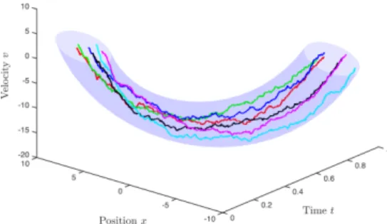
Figure 1 depicts the flow of the one-time marginals of the Schr¨odinger bridge with = 9. The transparent tube represents the
3σregion (ξ(t)0−m0t)Σ −1 t (ξ(t)−mt)≤9, ξ(t) = x(t) v(t)
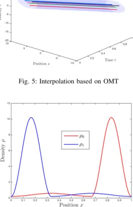
and the curves with different color stand for typical sample paths of the Schr¨odinger bridge. Similarly, Figures 2 and 3 depict the corresponding flows for = 4 and = 0.01, respectively. The interpolating flow in the absence of stochastic disturbance, i.e., for the optimal transport with prior, is depicted in Figure 4; the sample paths are now smooth as compared to the corresponding sample paths with stochastic disturbance. As&0, the paths converge to those corresponding to optimal transport and = 0. For comparison, we also provide in Figure 5 the interpolation corresponding to optimal transport without prior, i.e., for the trivial dynamicsA(t) ≡0and
B(t)≡I, which is precisely a constant speed translation.
B. General marginals
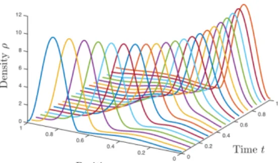
Consider now a large collection of particles obeying
Fig. 2: Interpolation based on Schr¨odinger bridge with= 4
Fig. 3: Interpolation based on Schr¨odinger bridge with= 0.01
in 1-dimensional state space with marginal distributions
ρ0(x) = ( 0.2−0.2 cos(3πx) + 0.2 if0≤x <2/3 5−5 cos(6πx−4π) + 0.2 if2/3≤x≤1, and ρ1(x) =ρ0(1−x).
These are shown in Figure 6 and, obviously, are not Gaussian. Once again, our goal is to steer the state of the system (equivalently, the particles) from the initial distribution ρ0 to the final ρ1 using minimum energy control. That is, we need to solve the problem of OMT-wpd. In this1-dimensional case, just like in the classical OMT
Fig. 4: Interpolation based on OMT-wpd
Fig. 5: Interpolation based on OMT
Fig. 6: Marginal distributions
problem, the optimal transport mapy=T(x)between the two end-points can be determined from7
Z x −∞ ρ0(y)dy= Z T(x) −∞ ρ1(y)dy.
The interpolation flowρt, 0 ≤ t≤ 1 can then be obtained using
(31). Figure 7 depicts the solution of OMT-wpd. For comparison, we also show the solution of the classical OMT in figure 8 where the particles move on straight lines.
Finally, we assume a stochastic disturbance,
dx(t) =−2x(t)dt+u(t)dt+√dw(t),
with >0. Figure 9–12 depict minimum energy flows for diffusion coefficients√= 0.5, 0.15, 0.05, 0.01, respectively. As→0, it is seen that the solution to the Schr¨odinger problem converges to the solution of the problem of OMT-wpd as expected.
VII. RECAP
The problem to steer the random state of a dynamical system between given probability distributions can be equally well be seen as the control problem to simultaneously herd a collection of particles obeying the given dynamics, or as the problem to identify a potential that effects such a transition. The former is seen to have applications 7In this 1-dimensional case, (30) is a simple rescaling and, therefore,T(·) inherits the monotonicity ofTˆ(·).
Fig. 7: Interpolation based on OMT-wpd
Fig. 8: Interpolation based on OMT
in the control of uncertain systems, system of particles, etc. The latter is seen as either a modeling or a system identification problem, where e.g., the collective response of particles is observed and the prior dynamics need to be adjusted by postulating a suitable potential so as to be consistent with observed marginals. When the dynamics are trivial (the state matrix is zero and the input matrix is the identity), the problem reduces to the classical OMT problem. Herein we presented a generalization to nontrivial linear dynamics. A version of both viewpoints where an added stochastic disturbance is present relates to the problem of constructing the so-called Schr¨odinger bridge between two end-point marginals. In fact, Schr¨odinger’s bridge problem was
Fig. 9: Interpolation based on Schr¨odinger bridge with√= 0.5
Fig. 10: Interpolation based on Schr¨odinger bridge with√= 0.15
Fig. 11: Interpolation based on Schr¨odinger bridge with√= 0.05
conceived as a modeling problem to identify a probability law on path space that is closest to a prior and is consistent with the marginals. Its stochastic control reformulation in the 90’s has led to a rapidly developing subject. The present work relates OMT as a limit to Schr¨odinger bridges, when the stochastic disturbance goes to zero, and discusses the generalization of both to the setting where the prior linear dynamics are quite general. It opens the way to employ the efficient iterative techniques recently developed for Schr¨odinger bridges [70] to the computationally challenging OMT (with or without prior dynamics). This is the topic of [58].
APPENDIX
A. Proof of Proposition 2
The velocity field associated withu(t, x) =B(t)0∇ψ(t, x)is
v(t, x) =A(t)x+B(t)B(t)0∇ψ(t, x),
which is well-defined almost everywhere (as it will be shown below thatψis indeed differentiable almost everywhere). Since we already know from previous discussion thatTt in (31b) gives the trajectories
associated with the optimal transportation plan, it suffices to show
v(t,·)◦Tt=dTt/dt,
that is, v(t, x) is the velocity field associated with the trajectories
(Tt)0≤t≤1. We next provev(t,·)◦Tt=dTt/dt.
For 0< t <1, formula (38) can be rewritten as
g(x) = sup y x0M(t,0)−1Φ(t,0)y−f(y) , with g(x) = 1 2x 0 M(t,0)−1x−ψ(t, x) f(y) = 1 2y 0 Φ(t,0)0M(t,0)−1Φ(t,0)y+ψ(0, y). The function f(y) = 1 2y 0 Φ(t,0)0M(t,0)−1Φ(t,0)y+ψ(0, y) = 1 2y 0 Φ(t,0)0M(t,0)−1Φ(t,0)−Φ010M10−1Φ10 y +φ(M10−1/2Φ10y)
is uniformly convex since φis convex and the matrix
Φ(t,0)0M(t,0)−1Φ(t,0)−Φ010M10−1Φ10 = Z t 0 Φ(0, τ)B(τ)B(τ)0Φ(0, τ)0dτ −1 − Z 1 0 Φ(0, τ)B(τ)B(τ)0Φ(0, τ)0dτ −1
is positive definite. Hence, f, g, ψ are differentiable almost ev-erywhere, and from a similar argument to the case of Legendre transform, we obtain
∇g◦(M(t,0)Φ(0, t)0∇f(x)) =M(t,0)−1Φ(t,0)x,
for allx∈Rn. It follows
(M(t,0)−1− ∇ψ(t,·))◦ M(t,0)Φ(0, t)0 × Φ(t,0)0M(t,0)−1Φ(t,0)x+∇ψ(0, x) =M(t,0)−1Φ(t,0)x.
After some cancellations it yields
∇ψ(t,·)◦Φ(t,0)x+∇ψ(t,·)◦M(t,0)Φ(0, t)0∇ψ(0, x)
−Φ(0, t)0∇ψ(0, x) = 0. (61) On the other hand, since
T(x) =M10−1/2∇φ(M10−1/2Φ10x) =M10Φ001∇ψ(0, x) + Φ10x, we have Tt(x) = Φ(t,1)M(1, t)M −1 10 Φ10x+M(t,0)Φ(1, t) 0 M10−1T(x) = (Φ(t,1)M(1, t) +M(t,0)Φ(0, t)0)M10−1Φ10x +M(t,0)Φ(0, t)0∇ψ(0, x) = Φ(t,0)x+M(t,0)Φ(0, t)0∇ψ(0, x).
The fact that(Φ(t,1)M(1, t) +M(t,0)Φ(0, t)0)M10−1Φ10= Φ(t,0)
follows by substituting expressions for the Grammians from (22). It now follows that
dTt(x) dt =A(t)Φ(t,0)x+A(t)M(t,0)Φ(0, t) 0 ∇ψ(0, x) +B(t)B(t)0Φ(0, t)0∇ψ(0, x). Therefore, v(t,·)◦Tt(x)− dTt(x) dt = A(t) +B(t)B(t)0∇ψ(t,·) ◦[Φ(t,0)x +M(t,0)Φ(0, t)0∇ψ(0, x) − A(t)Φ(t,0)x+A(t)M(t,0)Φ(0, t)0∇ψ(0, x) +B(t)B(t)0Φ(0, t)0∇ψ(0, x) =B(t)B(t)0{∇ψ(t,·)◦Φ(t,0)x +∇ψ(t,·)◦M(t,0)Φ(0, t)0∇ψ(0, x) −Φ(0, t)0∇ψ(0, x) = 0,
by (61), which completes the proof.
B. Proof of Theorem 3
The Markov kernel of (46) is
q(s, x, t, y) = (2π)−n/2|M(t, s)|−1/2 (62) ×exp −1 2(y−Φ(t, s)x) 0 M(t, s)−1(y−Φ(t, s)x) .
Comparing this and the Brownian kernelqB,we obtain
q(s, x, t, y) = (t−s)n/2|M(t, s)|−1/2
×qB,(s, M(t, s)−1/2Φ(t, s)x, t, M(t, s)−1/2y).
Now define two new marginal distributionsρ0ˆ and ρ1ˆ through the coordinates transformationCin (27), ˆ ρ0(x) = |M10|1/2| Φ10| −1 ρ0(Φ−101M 1/2 10 x), ˆ ρ1(x) = |M10|1/2 ρ1(M101/2x).
Let ( ˆϕ0, ϕ1) be a pair that solves the Schr¨odinger bridge problem with kernelq and marginalsρ0, ρ1, and define( ˆϕB0, ϕB1)as
ˆ ϕ0(x) = |Φ10|ϕˆB0(M −1/2 10 Φ10x), (63a) ϕ1(x) = |M10|−1/2ϕB1(M −1/2 10 x), (63b)
then the pair( ˆϕB
0, ϕB1) solves the Schr¨odinger bridge problem with
kernel qB, and marginals ρ0,ˆ ρ1ˆ. To verify this, we need only to show that the joint distribution
PB, 01 (E) = Z E qB,(0, x,1, y) ˆϕB0(x)ϕ B 1(y)dxdy
matches the marginalsρ0,ˆ ρ1ˆ. This follows from Z Rn qB,(0, x,1, y) ˆϕB0(x)ϕ B 1(y)dy = Z Rn qB,(0, x,1, M10−1/2y) ˆϕ B 0(x)ϕ B 1(M −1/2 10 y)d(M −1/2 10 y) =|M10|1/2|Φ10| −1Z Rn q(0,Φ−101M 1/2 10 x,1, y) ×ϕ0ˆ (Φ−101M 1/2 10 x)ϕ1(y)dy =|M10|1/2| Φ10| −1 ρ0(Φ−101M 1/2 10 x) = ˆρ0(x), and Z Rn qB,(0, x,1, y) ˆϕB0(x)ϕ B 1(y)dx = Z Rn qB,(0, M10−1/2Φ10x,1, y) ˆϕB0(M −1/2 10 Φ10x) ×ϕB1(y)d(M −1/2 10 Φ10x) =|M10|1/2 Z Rn q(0, x,1, M101/2y) ˆϕ0(x)ϕ1(M101/2y)dx =|M10|1/2ρ1(M101/2y) = ˆρ1(y). CompareP01B,withP
01it is not difficult to find out thatP
B,
01 is a
push-forward ofP
01, that is,
P01B,=C]P01.
On the other hand, letπB
be the solution to classical OMT (3) with marginalsρ0,ˆ ρ1ˆ, then πB =C]π. Now since PB, 01 weakly converge to π B from Theorem 2, we conclude that P
01 weakly converge toπasgoes to 0.
We next showP
t weakly converges toµtasgoes to 0 for all
t. The corresponding path space measureµcan be expressed as
µ(·) =
Z
Rn×Rn
δγxy(·)π(dxdy), whereγxy
is the minimum energy path (25) connectingx, y, andδγxy is the Dirac measure concentrated onγxy. Similarly, the Schr¨odinger bridge P can be decomposed [42] as P(·) = Z Rn×Rn Qxy(·)P 01(dxdy), whereQ
xy is the pinned bridge [73] (a generalization of Brownian
bridge) associated with (46) conditioned onx(0) =xand x(1) =
y, and it has the stochastic differential equation representation
dx(t) = (A(t)−B(t)B(t)0Φ(1, t)0M(1, t)−1Φ(1, t))x(t)dt
+B(t)B(t)0Φ(1, t)0M(1, t)−1ydt+√B(t)dw(t) (64) with initial value x(0) = x. As goes to zero, Q
xy tends to
concentrate on the solution of
dx0(t) = (A(t)−B(t)B(t)0Φ(1, t)0M(1, t)−1Φ(1, t))x0(t)dt
+B(t)B(t)0Φ(1, t)0M(1, t)−1ydt, x0(0) =x,
which isγxy. The linear stochastic differential equation (64) repre-sents a Gaussian process. It has the following explicit expression
x(t) =γxy(t) +√ Zt
0
˜
Φ(t, τ)B(τ)dw(τ), 0≤t <1, (65)
where Φ˜ is the transition matrix of the dynamics (64), and x(t)
converges to yalmost surely as tgoes to 1, see [73]. From (65) it is easy to see that the autocovariance of x(·)
depends linearly on
and therefore goes to0as→0. Combining this and the factx(·)
is a Gaussian process we conclude that the set of processes x(·)
is tight [74, Theorem 7.3] and their finite dimensional distributions converge weakly to those ofx0(·)
. Hence,Q
xyconverges weakly to
δγxy [74, Theorem 7.1] as goes to0. We finally claim thatP
t weakly converges toµt asgoes to
0for eacht. To see this, choose a bounded, uniformly continuous8 functionhand define
g(x, y) :=hQxy,t, hi,
g(x, y) :=hδγxy,t, hi
=h(γxy(t)),
where h·,·i denotes the integration of the function against the measure. From (25) it is immediate thatgis a bounded continuous functions ofx, y. Since Q
xy,t is a Gaussian distribution with mean
γxy(t)and covariance which is independent ofx, yand tends to zero as→0based on (65),g→guniformly as→0. It follows
hPt, hi − hµt, hi=hP01 , g i − hπ, gi = (hP 01, gi − hπ, gi) +hP 01, g − gi.
Both summands tend to zero as→0, the first due to weak conver-gence ofP
01 to πand the second due to the uniform convergence
ofgtog. This completes the proof.
ACKNOWLEDMENT
The authors are grateful to an anonymous referee for pointing out reference [15]. A second referee provided several constructive suggestions that have led to improvements in the exposition. They are also grateful to Markus Fischer for his input.
REFERENCES
[1] C. Villani,Topics in Optimal Transportation. American Mathematical Soc., 2003, no. 58.
[2] J.-D. Benamou and Y. Brenier, “A computational fluid mechanics so-lution to the Monge-Kantorovich mass transfer problem,”Numerische Mathematik, vol. 84, no. 3, pp. 375–393, 2000.
[3] L. V. Kantorovich, “On the transfer of masses,” inDokl. Akad. Nauk. SSSR, vol. 37, no. 7-8, 1942, pp. 227–229.
[4] W. Gangbo and R. J. McCann, “The geometry of optimal transportation,” Acta Mathematica, vol. 177, no. 2, pp. 113–161, 1996.
[5] R. Jordan, D. Kinderlehrer, and F. Otto, “The variational formulation of the Fokker–Planck equation,”SIAM journal on mathematical analysis, vol. 29, no. 1, pp. 1–17, 1998.
[6] S. T. Rachev and L. R¨uschendorf, Mass Transportation Problems: Volume I: Theory. Springer, 1998, vol. 1.
[7] L. C. Evans and W. Gangbo, Differential equations methods for the Monge-Kantorovich mass transfer problem. American Mathematical Soc., 1999, vol. 653.
[8] L. Ambrosio, N. Gigli, and G. Savar´e,Gradient flows: in metric spaces and in the space of probability measures. Springer, 2006.
8To guarantee weak convergence, it suffices to have bounded, uniform continuous test functions by Portmanteau Theorem [74].
[9] C. Villani,Optimal Transport: Old and New. Springer, 2008, vol. 338. [10] R. J. McCann and N. Guillen, “Five lectures on optimal transportation: geometry, regularity and applications,”Analysis and geometry of metric measure spaces: lecture notes of the s´eminaire de Math´ematiques Sup´erieure (SMS) Montr´eal, pp. 145–180, 2011.
[11] L. Ning, T. T. Georgiou, and A. Tannenbaum, “Matrix-valued Monge-Kantorovich optimal mass transport,” inDecision and Control (CDC), 2013 IEEE 52nd Annual Conference on. IEEE, 2013, pp. 3906–3911. [12] Y. Chen, T. T. Georgiou, and M. Pavon, “On the relation between optimal transport and schr¨odinger bridges: A stochastic control viewpoint,” Journal of Optimization Theory and Applications, pp. 1–21, 2014. [13] N. E. Leonard and E. Fiorelli, “Virtual leaders, artificial potentials
and coordinated control of groups,” in Decision and Control, 2001. Proceedings of the 40th IEEE Conference on, vol. 3. IEEE, 2001, pp. 2968–2973.
[14] S. Angenent, S. Haker, and A. Tannenbaum, “Minimizing flows for the Monge–Kantorovich problem,”SIAM journal on mathematical analysis, vol. 35, no. 1, pp. 61–97, 2003.
[15] R. W. Brockett, “Optimal control of the Liouville equation,”AMS IP Studies in Advanced Mathematics, vol. 39, p. 23, 2007.
[16] P. Dai Pra, “A stochastic control approach to reciprocal diffusion processes,”Applied mathematics and Optimization, vol. 23, no. 1, pp. 313–329, 1991.
[17] E. Schr¨odinger, “ ¨Uber die Umkehrung der Naturgesetze,” Sitzungs-berichte der Preuss Akad. Wissen. Phys. Math. Klasse, Sonderausgabe, vol. IX, pp. 144–153, 1931.
[18] E. Schr¨odinger, “Sur la th´eorie relativiste de l’´electron et l’interpr´etation de la m´ecanique quantique,” in Annales de l’institut Henri Poincar´e, vol. 2, no. 4. Presses universitaires de France, 1932, pp. 269–310. [19] A. Wakolbinger, “Schr¨odinger bridges from 1931 to 1991,” in Proc.
of the 4th Latin American Congress in Probability and Mathematical Statistics, Mexico City, 1990, pp. 61–79.
[20] R. Fortet, “R´esolution d’un syst`eme d’´equations de M. Schr¨odinger,”J. Math. Pures Appl., vol. 83, no. 9, 1940.
[21] A. Beurling, “An automorphism of product measures,”The Annals of Mathematics, vol. 72, no. 1, pp. 189–200, 1960.
[22] B. Jamison, “Reciprocal processes,”Z. Wahrscheinlichkeitstheorie verw. Gebiete, vol. 30, pp. 65–86, 1974.
[23] H. F¨ollmer, “Random fields and diffusion processes,” inEcole d’ ´´ Et´e de Probabilit´es de Saint-Flour XV–XVII, 1985–87. Springer, 1988, pp. 101–203.
[24] E. Nelson,Dynamical theories of Brownian motion. Princeton university press Princeton, 1967, vol. 17.
[25] E. Nelson,Quantum fluctuations. Princeton University Press Princeton, 1985.
[26] J. Zambrini, “Stochastic mechanics according to E. Schr¨odinger,” Phys-ical Review A, vol. 33, no. 3, p. 1532, 1986.
[27] B. C. Levy and A. J. Krener, “Stochastic mechanics of reciprocal diffusions,”Journal of Mathematical Physics, vol. 37, no. 2, pp. 769– 802, 1996.
[28] M. Pavon, “Quantum Schr¨odinger bridges,” inDirections in Mathemat-ical Systems Theory and Optimization. Springer, 2003, pp. 227–238. [29] S. Bernstein, “Sur les liaisons entre les grandeurs al´eatoires,” Verh.
Internat. Math.-Kongr., Zurich, pp. 288–309, 1932.
[30] A. J. Krener, “Reciprocal diffusions and stochastic differential equations of second order?”Stochastics: An International Journal of Probability and Stochastic Processes, vol. 24, no. 4, pp. 393–422, 1988.
[31] B. C. Levy, R. Frezza, and A. J. Krener, “Modeling and estimation of discrete-time gaussian reciprocal processes,”Automatic Control, IEEE Transactions on, vol. 35, no. 9, pp. 1013–1023, 1990.
[32] A. J. Krener, R. Frezza, and B. C. Levy, “Gaussian reciprocal pro-cesses and self-adjoint stochastic differential equations of second order,” Stochastics and stochastic reports, vol. 34, no. 1-2, pp. 29–56, 1991. [33] B. Levy and A. Krener, “Kinematics and dynamics of reciprocal
diffu-sions,”J. Math. Phys, vol. 34, no. 1846, p. 1875, 1993.
[34] F. P. Carli, A. Ferrante, M. Pavon, and G. Picci, “A maximum entropy solution of the covariance extension problem for reciprocal processes,” Automatic Control, IEEE Transactions on, vol. 56, no. 9, pp. 1999–2012, 2011.
[35] P. Dai Pra and M. Pavon, “On the Markov processes of Schr¨odinger, the Feynman–Kac formula and stochastic control,” inRealization and Modelling in System Theory. Springer, 1990, pp. 497–504.
[36] M. Pavon and A. Wakolbinger, “On free energy, stochastic control, and Schr¨odinger processes,” inModeling, Estimation and Control of Systems with Uncertainty. Springer, 1991, pp. 334–348.
[37] Y. Chen, T. T. Georgiou, and M. Pavon, “Optimal steering of a linear stochastic system to a final probability distribution, Part I,” arXiv:1408.2222,IEEE Trans. on Automatic Control, to appear, 2016. [38] Y. Chen, T. T. Georgiou, and M. Pavon, “Optimal steering of a linear stochastic system to a final probability distribution, Part II,” arXiv:1410.3447,IEEE Trans. on Automatic Control, to appear, 2016. [39] Y. Chen, T. T. Georgiou, and M. Pavon, “Optimal steering of inertial par-ticles diffusing anisotropically with losses,” inProc. American Control Conf. (arXiv:1410.1605v1), 2015, pp. 1252–1257.
[40] Y. Chen, T. T. Georgiou, and M. Pavon, “Fast cooling for a system of stochastic oscillators,”Journal of Mathematical Physics, vol. 56, no. 11, p. 113302, 2015.
[41] C. L´eonard, “From the Schr¨odinger problem to the Monge–Kantorovich problem,”Journal of Functional Analysis, vol. 262, no. 4, pp. 1879– 1920, 2012.
[42] C. L´eonard, “A survey of the Schr¨odinger problem and some of its connections with optimal transport,” Dicrete Contin. Dyn. Syst. A, vol. 34, no. 4, pp. 1533–1574, 2014.
[43] T. Mikami, “Monge’s problem with a quadratic cost by the zero-noise limit of h-path processes,”Probability theory and related fields, vol. 129, no. 2, pp. 245–260, 2004.
[44] T. Mikami and M. Thieullen, “Optimal transportation problem by stochastic optimal control,”SIAM Journal on Control and Optimization, vol. 47, no. 3, pp. 1127–1139, 2008.
[45] R. Brockett, “Notes on the control of the liouville equation,” inControl of Partial Differential Equations. Springer, 2012, pp. 101–129. [46] A. Hindawi, J.-B. Pomet, and L. Rifford, “Mass transportation with LQ
cost functions,”Acta applicandae mathematicae, vol. 113, no. 2, pp. 215–229, 2011.
[47] R. J. McCann, “A convexity principle for interacting gases,”Advances in mathematics, vol. 128, no. 1, pp. 153–179, 1997.
[48] Y. Brenier, “Polar factorization and monotone rearrangement of vector-valued functions,”Communications on pure and applied mathematics, vol. 44, no. 4, pp. 375–417, 1991.
[49] J.-D. Benamou, B. D. Froese, and A. M. Oberman, “Numerical solution of the optimal transportation problem using the Monge-Ampere equa-tion,”Journal of Computational Physics, vol. 260, pp. 107–126, 2014. [50] A. Figalli, Optimal transportation and action-minimizing measures.
Publications of the Scuola Normale Superiore, Pisa, Italy, 2008. [51] P. Bernard and B. Buffoni, “Optimal mass transportation and Mather
theory,”J. Eur. Math. Soc., vol. 9, pp. 85–121, 2007.
[52] W. Fleming and R. Rishel,Deterministic and Stochastic Optimal Con-trol. Springer, 1975.
[53] E. B. Lee and L. Markus,Foundations of optimal control theory. Wiley, 1967.
[54] M. Athans and P. Falb,Optimal Control: An Introduction to the Theory and Its Applications. McGraw-Hill, 1966.
[55] W. H. Fleming and H. M. Soner, Controlled Markov processes and viscosity solutions. Springer Science & Business Media, 2006, vol. 25. [56] M. G. Crandall, H. Ishii, and P.-L. Lions, “User’s guide to viscosity solutions of second order partial differential equations,”Bulletin of the American Mathematical Society, vol. 27, no. 1, pp. 1–67, 1992. [57] L. C. Evans, Partial differential equations. American Mathematical
Soc., 1998, vol. 19.
[58] Y. Chen, T. T. Georgiou, and M. Pavon, “Entropic and displace-ment interpolation: a computational approach using the hilbert metric,” arXiv:1506.04255v1, 2015.
[59] A. Blaqui`ere, “Controllability of a Fokker-Planck equation, the Schr¨odinger system, and a related stochastic optimal control (revised version),”Dynamics and Control, vol. 2, no. 3, pp. 235–253, 1992. [60] R. Van Handel, “Stochastic calculus, filtering, and stochastic control,”
Course notes., URL http://www. princeton. edu/˜ rvan/acm217/ACM217. pdf, 2007.
[61] I. Karatzas and S. Shreve,Brownian Motion and Stochastic Calculus. Springer, 1988.
[62] I. Gentil, C. L´eonard, and L. Ripani, “About the analogy between optimal transport and minimal entropy,”arXiv:1510.08230, 2015.
[63] E. Carlen, “Stochastic mechanics: a look back and a look ahead,” in Diffusion, Quantum Theory and Radically Elementary Mathematics, W. G. Faris, Ed. Princeton University Press, 2006, vol. 47, pp. 117–139. [64] A. Dembo and O. Zeitouni,Large deviations techniques and
applica-tions. Springer Science & Business Media, 2009, vol. 38.
[65] N. Ikeda and S. Watanabe,Stochastic differential equations and diffusion processes. Elsevier, 2014.
[66] S. Kullback and R. A. Leibler, “On information and sufficiency,”The annals of mathematical statistics, vol. 22, no. 1, pp. 79–86, 1951. [67] M. Fischer, “Markov processes and martingale problems,”
http://www.math.unipd.it/˜fischer/Didattica/MarkovMP.pdf, 2012, notes for a graduate course in mathematics, University of Padua.
[68] A. Wakolbinger, “A simplified variational characterization of Schr¨odinger processes,” Journal of mathematical physics, vol. 30, no. 12, pp. 2943–2946, 1989.
[69] S. N. Ethier and T. G. Kurtz,Markov processes: characterization and convergence. John Wiley & Sons, 2009, vol. 282.
[70] T. T. Georgiou and M. Pavon, “Positive contraction mappings for classical and quantum Schr¨odinger systems,” J. Math. Phys. (arXiv:1405.6650v2), vol. 56, p. 033301, 2015.
[71] M. Cuturi, “Sinkhorn distances: Lightspeed computation of optimal transport,” inAdvances in Neural Information Processing Systems, 2013, pp. 2292–2300.
[72] J.-D. Benamou, G. Carlier, M. Cuturi, L. Nenna, and G. Peyr´e, “Iterative bregman projections for regularized transportation problems,” SIAM Journal on Scientific Computing, vol. 37, no. 2, pp. A1111–A1138, 2015. [73] Y. Chen and T. T. Georgiou, “Stochastic bridges of linear systems,” arXiv:1407.3421,IEEE Trans. on Automatic Control,to appear, 2016.
[74] P. Billingsley,Convergence of probability measures. John Wiley & Sons, 1999.
Yongxin Chen received his BSc in Mechanical Engineering from Shanghai Jiao Tong university, China, in 2011. He obtained his Ph.D. in Mechanical Engineering from University of Minnesota in 2016 under the supervision of Tryphon Georgiou, with a Ph.D. minor in Mathematics. He is now a postdoc fellow in the Department of Electrical and Computer Engineering in University of Minnesota. He is interested in the application of mathematics in engineering and theoretical physics. His current research focuses on linear dynamical systems, stochastic processes and optimal mass transport theory. Tryphon T. Georgiou received the Diploma in Mechanical and Electrical Engineering from the National Technical University of Athens, Greece, in 1979 and the Ph.D. degree from the University of Florida, Gainesville, in 1983. He is a faculty in the Department of Electrical and Computer Engineering at the University of Minnesota and the Vincentine Hermes-Luh Chair. He is a recipient of the George S. Axelby Outstanding Paper award of the IEEE Control Systems Society for the years 1992, 1999, and 2003, a Fellow of the Institute of Electrical and Electronic Engineers (IEEE), and a Foreign Member of the Royal Swedish Academy of Engineering Sciences (IVA). Michele Pavonwas born in Venice, Italy, on October 12, 1950. He received the Laurea degree from the University of Padova, Padova, Italy, in 1974, and the Ph.D. degree from the University of Kentucky, Lexington, in 1979, both in mathematics. After service in the Italian Army, he was on the research staff of LADSEB-CNR, Padua, Italy, for six years.Since July 1986, he has been a Professor at the School of Engineering, the University of Padova. He has visited several institutions in Europe, Northern America and Asia. His present research interests include maximum entropy and optimal transport problems.