A quantile-copula approach to conditional density estimation

Contents lists available atScienceDirect

Journal of Multivariate Analysis

journal homepage:www.elsevier.com/locate/jmva

A quantile-copula approach to conditional density estimation

Olivier P. Faugeras

L.S.T.A., Université Paris 6, 175, rue du Chevaleret, 75013 Paris, France

a r t i c l e i n f o

Article history: Received 4 January 2008 Available online 26 March 2009 AMS 1991 subject classifications: 62G007 62M20 62M10 Keywords: Copula Conditional density Kernel estimation Nonparametric regression Quantile transform

a b s t r a c t

A new kernel-type estimator of the conditional density is proposed. It is based on an efficient quantile transformation of the data. The proposed estimator, which is based on the copula representation, turns out to have a remarkable product form. Its large-sample properties are considered and comparisons in terms of bias and variance are made with competitors based on nonparametric regression. A comparative simulation study is also provided.

©2009 Elsevier Inc. All rights reserved.

1. Introduction 1.1. Motivation

Let

(

X1

,

Y1

), . . . , (

Xn

,

Yn

)

be mutually independent copies of a pair

(

X

,

Y

)

of random variables. In many applications, it is of interest to estimate the conditional densityf

(

y

|

x

)

, not just its mean. Knowledge concerning the general shape off

(

y

|

x

)

is especially important for prediction purposes when the conditional distribution is multimodal or skewed, as often arises in non-linear or non-Gaussian phenomena. In those circumstances, the conditional expectation might be nowhere near a mode. Needless to say, the estimated conditional density is also useful for the construction of confidence intervals. 1.2. Estimation by kernel smoothing

A natural starting point for the estimation off

(

y

|

x

)

is the identity f

(

y

|

x

)

=

fXY

(

x

,

y

)

fX

(

x

)

,

(1)

in whichfXY andfXdenote the joint density of

(

X

,

Y

)

andX, respectively. Parzen–Rosenblatt kernel estimators of the latter are given by

ˆ

fn,XY

(

x

,

y

)

=

1 n n

X

i=1 K_h00

(

Xi

−

x

)

Kh

(

Yi

−

y

),

ˆ

fn,X

(

x

)

=

1 n n

X

i=1 K_h00

(

Xi

−

x

),

E-mail address:[email protected].

0047-259X/$ – see front matter©2009 Elsevier Inc. All rights reserved.

respectively. Here,Kh

(

·

)

=

1

/

hK

(

·

/

h

)

andKh00

(

·

)

=

1

/

h0K0

(

·

/

h0

)

are (rescaled) kernels whose associated sequencesh

=

hn andh0

₌

_h0

nof bandwidth vanish asn

→ ∞

. Accordingly, an estimator off

(

y

|

x

)

is given by

ˆ

f_nR

(

y

|

x

)

=

ˆ

fn,XY

(

x

,

y

)

ˆ

fn,X

(

x

)

.

This estimator was originally introduced by Rosenblatt [1]; see Hyndman et al. [2] for a recent improvement. 1.3. Estimation by regression techniques

As pointed out by numerous authors (see, e.g., Chapter 6 of Fan and Yao [3]), the kernel-smoothing approach to estimation off

(

y

|

x

)

can be expressed equivalently in a regression framework. To see this, observe that ifF

(

y

|

x

)

is the cumulative distribution function (c.d.f.) ofYgivenX

=

x, then ash

→

0,

E 1|Y−y|≤h

|

X

=

x

=

F

(

y

+

h

|

x

)

−

F

(

y

−

h

|

x

)

≈

2hf

(

y

|

x

).

Thus if the expectation in the above expression is replaced by its empirical counterpart, one can apply the usual local averaging methods and perform a regression estimation on the synthetic data1|Y1−y|≤h

/(

2h

), . . . ,

1|Yn−y|≤h

/(

2h

)

. A

Bochner-type theorem can also be invoked to justify the use of smoothed transformed data, viz. Y_i0

=

Kh

(

Yi

−

y

)

=

1 hK

Yi

−

y h

.

In particular, the popular Nadaraya–Watson regression estimator

ˆ

f_nNW

(

y

|

x

)

=

n

P

i=1 Y0 iK 0 h0

(

Xi

−

x

)

n

P

i=1 K0 h0

(

Xi

−

x

)

reduces to the same estimator as above, viz.

ˆ

f_nNW

(

y

|

x

)

=

n

P

i=1 Kh

(

Yi

−

y

)

K_h00

(

Xi

−

x

)

n

P

i=1 K0 h0

(

Xi

−

x

)

= ˆ

f_nR

(

y

|

x

).

Taking advantage of this regression formulation, Fan et al. [4] generalized the kernel-based estimate of the conditional density using local polynomial techniques. This makes it possible to tackle the bias issues associated with kernel smoothing. However, this is at the cost of an estimator that may take negative values and that does not always integrate to 1 with respect toy. This led Hyndman and Yao [5] to propose alternative solutions built on local polynomial techniques: one is based on a local fit of a log-linear model; the other involves constrained local polynomial modeling. An overview can be found in Chapters 6 and 10 of Fan and Yao [3]. More recently, Györfi and Kohler [6] considered a partitioning-type estimate and Lacour [7] proposed a projection-type estimate for Markov chains. Minimax rates of convergence were also obtained by Efromovich [8].

1.4. A product-shaped estimator

The kernel-based approach described above suffers from several drawbacks. From a practical point of view, the Nadaraya–Watson estimator (and its local polynomial counterpart) may be numerically unstable when the denominator is close to zero. The large-sample behavior of the estimators is also difficult to track down, due to the quotient form. This problem is usually addressed by linearizing the inverse after centering the numerator and the denominator individually; see, e.g., [3] or [9] for details. At a conceptual level, one could also argue that implementing regression estimation techniques in this setting is somewhat artificial: estimating a density, albeit a conditional one, should resort to density estimation techniques only.

To remedy these problems, we propose an estimator which builds on the idea of using pseudo-observations, i.e., a transformation of the original data. To be specific, a quantile transform of the data will be seen to lead, through a copula representation, to a product-form estimator

ˆ

fn

(

y

|

x

)

= ˆ

fY

(

y

)

c

ˆ

n

{

Fn

(

x

),

Gn

(

y

)

}

wheref

ˆ

Y,

ˆ

cn,Fn

(

x

)

,Gn

(

y

)

are estimators of the densityfYofY, the copula densityc, the c.d.f.FofXandGofY, respectively. As will be shown, the properties of

ˆ

fn

(

y

|

x

)

are easily deduced from existing results in nonparametric density estimation.

The rest of the paper is organized as follows. The quantile transform and the copula representation leading to the proposed estimator are introduced in Section2. The asymptotic properties of the estimator are studied in Section3and compared in Section4to those of various competitors. Technical arguments are deferred toAppendix.

2. Presentation of the estimator 2.1. The quantile transform

Data transformations are common. They are often used to improve the range of applicability and performance of classical estimation techniques to deal with skewed data, heavy tails, or restrictions on the support, among others; see, e.g., Chapter 14 of Devroye and Lugosi [10]. In order to make inference onY fromX, an appropriate choice of transformation must be made. We will see below that, in our context, a natural candidate is the quantile transform, i.e., the mappingX

7→

U

=

F

(

X

)

which turns a continuous random variableXwith c.d.f.Finto a uniform random variableUon the interval

[

0

,

1

]

.

2.2. The copula representation

A copula is a cumulative distribution function whose margins are uniform on the interval

[

0

,

1

]

. Sklar [11] proved the following fundamental result:

Theorem 2.1. For any bivariate c.d.f. FX,YonR2, with marginal c.d.f. F of X and G of Y , there exists some function C

: [

0

,

1

]

2

→

[

0

,

1

]

, called the dependence or copula function, such as

FX,Y

(

x

,

y

)

=

C

{

F

(

x

),

G

(

y

)

}

,

−∞ ≤

x

,

y

≤ +∞

.

(2)

If F and G are continuous, this representation is unique. The copula C is itself a c.d.f. on

[

0

,

1

]

2_{with uniform margins.}

This theorem gives a representation of the bivariate c.d.f. as a function of each univariate c.d.f. In other words, the copula captures the dependence structure in the pair

(

X

,

Y

)

, irrespectively of the marginal distributionFandG. Simply put, it allows one to deal with the randomness of the dependence structure and the randomness of the margins separately.

Copulas are naturally linked with the quantile transform as formula(2)entails thatC

(

u

, v)

=

FX,Y

{

F−1

(

u

),

G−1

(v)

}

. For more details regarding copulas and their properties, see, e.g., the book of Joe [12]. As described, e.g., by Genest et al. [13], copulas have gained popularity in statistics, especially in finance, since the pioneering work of Rüschendorf [14], who studied the properties of the empirical copula process; see also Deheuvels [15], van der Vaart and Wellner [16], Fermanian et al. [17] and Tsukahara [18]. For the estimation of the copula density, refer, e.g., to Gijbels and Mielniczuk [19], Fermanian [20], Fermanian and Scaillet [21] or Genest et al. [22].

From now on, we assume that the copula functionC

(

u

, v)

has a density c

(

u

, v)

=

∂

2

∂

u

∂v

C

(

u

, v)

with respect to the Lebesgue measure on

[

0

,

1

]

2_{and thatFandGare strictly increasing and differentiable with densitiesfand}

g.C

(

u

, v)

andc

(

u

, v)

are then the c.d.f. and density of the transformed variables

(

U

,

V

)

=

(

F

(

X

),

G

(

Y

))

. Upon differentiating both sides of(2), we get the joint density, viz.

fXY

(

x

,

y

)

=

∂

2

∂

x

∂

yFXY

(

x

,

y

)

=

f

(

x

)

g

(

y

)

c

{

F

(

x

),

G

(

y

)

}

.

This leads to the following explicit formula of the conditional density: fY|X

(

x

,

y

)

=

fXY

(

x

,

y

)

f

(

x

)

=

g

(

y

)

c

{

F

(

x

),

G

(

y

)

}

.

(3)

2.3. Construction of the estimator

Starting from the previously stated product-type formula(3), a natural plug-in approach to build an estimator of the conditional density is using:

•

a Parzen–Rosenblatt kernel-type nonparametric estimator of the densitygofY, viz.

ˆ

gn

(

y

)

=

1 nhn n

X

i=1 K0

y

−

Yi hn

;

•

the empirical counterparts ofFandG, viz. Fn

(

x

)

=

1 n n

X

j=1 1Xj≤x and Gn

(

y

)

=

1 n n

X

j=1 1Yj≤y

.

Given thatc

(

u

, v)

is the joint density of the transformed variables

(

U

,

V

)

=

(

F

(

X

),

G

(

Y

))

, it could be estimated in principle by the bivariate Parzen–Rosenblatt kernel-type nonparametric density (pseudo) estimator,

cn

(

u

, v)

=

1 nanbn n

X

i=1 K

u

−

Ui an

,

v

−

Vi bn

,

(4)

whereKis a bivariate kernel andan,bnits associated bandwidths. For simplicity, we restrict ourselves to product kernels, i.e.,K

(

u

, v)

=

K1

(

u

)

K2

(v)

with the same bandwidthan

=

bn.

BecauseFandGare unknown, however, the random variables

(

U1

,

V1

)

,

. . .

,

(

Un

,

Vn

)

are not observable, i.e.,cnis not a feasible solution. Therefore, we approximate

(

Ui

,

Vi

)

by its empirical counterpart

(

Fn

(

Xi

),

Gn

(

Yi

))

,i

=

1

, . . . ,

n. Thus we obtain a rank-based estimator ofc

(

u

, v)

, viz.

ˆ

cn

(

u

, v)

=

1 na2 n n

X

i=1 K1

u

−

Fn

(

Xi

)

an

K2

v

₋

Gn

(

Yi

)

an

.

(5)

Accordingly, the conditional density estimator is written as

ˆ

fn

(

y

|

x

)

=

(

1 nhn n

X

i=1 K0

y

−

Yi hn

) (

1 na2 n n

X

i=1 K1

Fn

(

x

)

−

Fn

(

Xi

)

an

K2

Fn

(

y

)

−

Gn

(

Yi

)

an

)

or more compactly in the form

ˆ

fn

(

y

|

x

)

= ˆ

gn

(

y

)

ˆ

cn

{

Fn

(

x

),

Gn

(

y

)

}

.

(6)

Remark 1. To our knowledge, the estimator studied in this paper is new. However, connections can be made with the nearest-neighbor estimator proposed by Stute [23–25] for conditional c.d.f., as well as with the estimators of Gasser and Müller [26] and Priestley and Chao [27] in the context of regression estimation. Indeed, these estimators circumvent the random denominator issue by first transforming the designX1

, . . . ,

Xnto a uniform (random) one. This results in assigning the surfaces under the kernel function instead of its heights as weights. Contrary to our estimator, they do not make transformations of the data in both directionsXandY.

3. Asymptotic results

3.1. Notations and assumptions

We note theith moment of a generic (possibly multivariate) kernelK asmi

(

K

)

=

R

uiK

(

u

)

du, and theLpnorm of a functionhby

k

h

k

_p

=

R

hp_{. We use the symbol}

_'

_{to denote the order of the bandwidths, i.e.,h}

n

'

unmeans thathn

=

cnun withcn

→

c

>

0. We also denote supp

(

f

)

= {

x

∈

R

;

f

(

x

) >

0

}

and supp

(

c

)

= {

(

u

, v)

∈

R2

;

c

(

u

, v) >

0

}

, respectively.

To obtain our results, we will have to impose regularity assumptions on the kernels and the densities which, although far from being minimal, are customary in kernel density estimation. Letxandybe fixed points in the interior of supp

(

f

)

and supp

(

g

)

, respectively. In the remainder of this paper, we suppose that

(i) the c.d.f.FofXandGofYare strictly increasing and differentiable;

(ii) the densitiesgandcare twice differentiable with continuous bounded second derivatives on their support. Moreover, we assume that the kernelsK0andKsatisfy the following:

(i) KandK0are of bounded support and of bounded variation;

(ii) 0

≤

K

≤

Cand 0

≤

K0

≤

Cfor some constantC;

(iii) KandK0are first-order kernels:m0

(

K

)

=

1,m1

(

K

)

=

0 andm2

(

K

) <

+∞

, and the same forK0.

In order to approximatec

ˆ

nbycn, we will also impose that the bivariate kernelKis twice differentiable with bounded second partial derivatives.

3.2. Weak and strong consistency of the estimator

Theorem 3.1. Let the regularity conditions on the densities and kernels be satisfied, if max

(

hn

,

an

)

→

0as n

→ ∞

in such a way that nhn

→ ∞

,

na4n

→ ∞

,

na 3 n

/

√

ln lnn

→ ∞

then

ˆ

fn

(

y

|

x

)

=

f

(

y

|

x

)

+

OP 1

√

nhn

+

h2_n

+

1

p

na2 n

+

a2_n

!

.

Proof. Recall from(4)and(5)thatcnandc

ˆ

nare estimators ofcbased on the unobservable pseudo-data

(

F

(

Xi

),

G

(

Yi

))

and their approximations

(

Fn

(

Xi

),

Gn

(

Yi

))

, respectively. The main ingredient of the proof is the decomposition:

ˆ

fn

(

y

|

x

)

−

f

(

y

|

x

)

= ˆ

gn

(

y

)

c

ˆ

n

{

Fn

(

x

),

Gn

(

y

)

} −

g

(

y

)

c

{

F

(

x

),

G

(

y

)

}

=

g

ˆ

n

(

y

)

−

g

(

y

)

c

ˆ

n

{

Fn

(

x

),

Gn

(

y

)

} +

g

(

y

)

ˆ

cn

{

Fn

(

x

),

Gn

(

y

)

} −

c

{

F

(

x

),

G

(

y

)

}

=

D1

+

D2

.

We proceed one step further in the decomposition of each term, by centering at fixed locations, viz. D1

=

ˆ

gn

(

y

)

−

g

(

y

)

ˆ

cn

{

Fn

(

x

),

Gn

(

y

)

} − ˆ

cn

{

F

(

x

),

G

(

y

)

}

+

g

ˆ

n

(

y

)

−

g

(

y

)

ˆ

cn

{

F

(

x

),

G

(

y

)

} −

cn

{

F

(

x

),

G

(

y

)

}

+

g

ˆ

n

(

y

)

−

g

(

y

)

[cn

{

F

(

x

),

G

(

y

)

} −

c

{

F

(

x

),

G

(

y

)

}

]

+

ˆ

gn

(

y

)

−

g

(

y

)

[c

{

F

(

x

),

G

(

y

)

}

] (7) D2

=

g

(

y

)

ˆ

cn

{

Fn

(

x

),

Gn

(

y

)

} − ˆ

cn

{

F

(

x

),

G

(

y

)

}

+

g

(

y

)

c

ˆ

n

{

F

(

x

),

G

(

y

)

} −

cn

{

F

(

x

),

G

(

y

)

}

+

g

(

y

)

[c_n

{

F

(

x

),

G

(

y

)

} −

c

{

F

(

x

),

G

(

y

)

}

]

.

(8)

In view ofLemmas A.2andA.3, one has

ˆ

gn

(

y

)

−

g

(

y

)

=

Op

(

h2n

+

1

/

p

nhn

)

and cn

{

F

(

x

),

G

(

y

)

} −

c

{

F

(

x

),

G

(

y

)

} =

Op

(

a2n

+

1

/

q

na2 n

).

ApproximationLemmas A.4andA.5further entail that

ˆ

cn

{

F

(

x

),

G

(

y

)

} −

cn

{

F

(

x

),

G

(

y

)

} =

OP n−1/2

+

√

ln lnn na3 n

+

1 na4 n

!

ˆ

cn

{

Fn

(

x

),

Gn

(

y

)

} − ˆ

cn

{

F

(

x

),

G

(

y

)

} =

OP

n−1/2

+

1 na4 n

.

We therefore conclude that

D1

= { ˆ

gn

(

y

)

−

g

(

y

)

}[

c

{

F

(

x

),

G

(

y

)

} +

oP

(

1

)

] =

OP

h2_n

+

1

/

p

nhn

,

D2

=

g

(

y

)

OP a2n

+

1

p

na2 n

+

1 na4 n

+

√

ln lnn na3 n

!

,

which entails the convergence of the estimator, provided the bandwidths satisfy the above-mentioned conditions.

Remark 2. As a corollary, we get the rate of convergence, by choosing the bandwidths which balance the bias and variance trade-off: for an optimal choice ofhn

'

n−1/5andan

'

n−1/6, we get

ˆ

f

(

y

|

x

)

=

f

(

y

|

x

)

+

OP

(

n−1/3

).

Therefore, our estimator is rate-optimal in the sense that it reaches the minimax raten−1/3_{of convergence, according to}

Efromovich [8].

Almost sure results can be proved in the same way, we have the following strong consistency result.

Theorem 3.2. Let the regularity conditions on the densities and kernels be satisfied. If max

(

hn

,

an

)

→

0as n

→ ∞

in such a way that nhn ln lnn

→ ∞

,

(

lnnln lnn

)

1/2 na3 n

→

0

,

ln lnn na4 n

→

0

then

ˆ

fn

(

y

|

x

)

=

f

(

y

|

x

)

+

Oa.s. a2n

+

s

ln lnn na2 n

+

h2_n

+

s

ln lnn nhn

+

ln lnn na4 n

+

√

lnnln lnn na3 n

!

.

Proof. It follows the same lines as the preceding theorem, but uses the a.s. results of the consistency of the kernel density estimators ofLemmas A.2andA.3, as well as the approximationLemmas A.4andA.5. It is therefore omitted.

Remark 3. Forhn

'

(

ln lnn

/

n

)

1/5andan

'

(

ln lnn

/

n

)

1/6, which is the optimal trade-off between the bias and the stochastic term, one gets the optimal rate

(

ln lnn

/

n

)

1/3_.

3.3. Convergence in distribution

Theorem 3.3. Let the regularity conditions on the densities and kernels be satisfied. If max

(

hn

,

an

)

→

0as n

→ ∞

in such a way that nhn

→ ∞

,

√

ln lnn na3 n

,

na4_n

→ ∞

,

na6_n

→

0

,

then

q

na2 n

{ˆ

fn

(

y

|

x

)

−

f

(

y

|

x

)

}

N 0

,

g

(

y

)

f

(

y

|

x

)

k

K

k

22

.

Proof. With the conditions on the bandwidths, all the terms in decomposition(7)and (8)are negligible compared to

(

na2

n

)

−1/2_exceptc

n

{

F

(

x

),

G

(

y

)

} −

c

{

F

(

x

),

G

(

y

)

}

, which is asymptotically normal byLemma A.3, provided that asn

→ ∞

, an

→

0,na2n

→ ∞

,na6n

→

0 and

q

na2 ng

(

y

)

[cn

{

F

(

x

),

G

(

y

)

} −

c

{

F

(

x

),

G

(

y

)

}

] N 0

,

g2

(

y

)

c

{

F

(

x

),

G

(

y

)

} k

K

k

22

.

An application of Slutsky’s Lemma yields the desired result.

For a vector

(

y1

, . . . ,

yd

)

, one can get a multidimensional version of the convergence in distribution (fidi convergence):

Corollary 3.4. With the same assumptions, for

(

y1

, . . . ,

yd

)

in the interior of supp

(

g

)

such that g

(

yi

)

f

(

yi

|

x

)

6=

0,

q

na2 n

(

ˆ

fn

(

yi

|

x

)

−

f

(

yi

|

x

)

√

g

(

yi

)

f

(

yi

|

x

)

k

K

k

2

)

,

i

=

1

, . . . ,

m

!

N(m)

,

whereN(m)_{is the standard m-variate centered normal distribution with identity variance matrix.}

Proof. It simply follows from the use of the Cramér–Wold device and is therefore omitted. For details, see, e.g., Theorem 2.3 in [9].

3.4. Asymptotic bias, variance and mean square error

The asymptotic bias is calculated in the following proposition. Proposition 3.5. Under the assumptions ofTheorem3.1, we have

B0

=

E

{ˆ

fn

(

y

|

x

)

} −

f

(

y

|

x

)

=

g

(

y

)

BK

(

c

,

x

,

y

)

a2n

/

2

+

o

(

a

2

n

)

with BK

(

c

,

x

,

y

)

=

m2

(

K1

)∂

2c

{

F

(

x

),

G

(

y

)

}

/∂

u2

+

m2

(

K2

)∂

2c

{

F

(

x

),

G

(

y

)

}

/∂v

2.

Proof (Sketch). By taking expectation in decomposition(7)and(8), one can write ED1

=

c

{

F

(

x

),

G

(

y

)

}

E

{ ˆ

gn

(

y

)

−

g

(

y

)

} +

R1

,

ED2

=

g

(

y

)

E

(

[

cn

{

F

(

x

),

G

(

y

)

} −

c

{

F

(

x

),

G

(

y

)

}]

)

+

R2

,

whereR1andR2stand for the remaining terms. With the assumptions on the bandwidths, and through tedious derivations

caused by the transformation of the data through the empirical margins (see Theorem 1 of Fermanian [20] for such a

calculation), the terms inR2may be shown to be negligible compared to the bias ofcn. The bias ofcn, which is simply the bias of a bivariate kernel density estimator, is of ordera2

n. Similarly, by bounding the product terms inD1by the Cauchy–Schwarz

inequality, routine analysis shows that the terms inR1are negligible compared to the bias ofg

ˆ

n, which is of orderh2n. Sinceh2n is itself negligible toa2_n, the main term in the decomposition isg

(

y

)

E

[

cn

{

F

(

x

),

G

(

y

)

}−

C

{

F

(

x

),

G

(

y

)

}]

. Plugging the expression of the bias given inLemma A.3yields the desired result.

The asymptotic variance has already been derived inTheorem 3.3, viz. V0

=

var

{ˆ

f

(

y

|

x

)

} =

1

/(

na2n

)

g

(

y

)

f

(

y

|

x

)

k

K

k

2 2

+

o

(

1

/(

na 2 n

)).

Together with the computation of the asymptotic bias, we get the asymptotic mean squared error as a corollary. Corollary 3.6. With the previous assumptions, the Asymptotic Mean Squared Error (AMSE) E0at

(

x

,

y

)

is

E0

=

B20

+

V0

,

=

a 4 ng2

(

y

)

{

Bk

(

c

,

x

,

y

)

}

2 4

+

g

(

y

)

f

(

y

|

x

)

k

K

k

2 2 na2 n

+

o

a4_n

+

1 na2 n

,

which gives, for the choice of the usual bandwidths mentioned above, E0

=

n−2/3g2

(

y

)

B2 K

(

c

,

x

,

y

)

4

+

c

{

F

(

x

),

G

(

y

)

}k

K

k

2 2

+

o

(

n−2/3

).

4. Comparison with other estimators

4.1. Presentation of alternative estimators

For convenience, we recall below the definition of alternative estimators of the conditional density and summarize their bias and variance properties. The bias and variance off

ˆ

_ni

(

y

|

x

)

are denoted byEiandVi, respectively.

(1) Double kernel estimator: It was defined in the Introduction by

ˆ

f_n(1)

(

y

|

x

)

=

1 n n

P

i=1 K0 h1

(

Xi

−

x

)

Kh2

(

Yi

−

y

)

1 n n

P

i=1 K0 h1

(

Xi

−

x

)

,

whereh1andh2are the bandwidths. One then has (see, e.g., [2])

B1

=

h2₁m2

(

K

)

2

(

2f 0

₍

x

)

f

(

x

)

∂

∂

xf

(

y

|

x

)

+

∂

2

∂

x2f

(

y

|

x

)

+

h2 h1

2

∂

2

∂

y2f

(

y

|

x

)

)

+

o h2₁

+

h2₂

and V1

=

k

K

k

2 2f

(

y

|

x

)

nh1h2f

(

x

)

k

K

k

2 2

−

h2f

(

y

|

x

)

+

o

1 nh1h2

.

(2) Local polynomial estimator: Set R

(θ,

x

,

y

)

=

n

X

i=1

(

Kh2

(

Yi

−

y

)

−

r

X

j=0

θ

j

(

Xi

−

x

)

j

)

2 K_h0₁

(

Xi

−

x

).

The local polynomial estimator is then defined asf

ˆ

n(2)

(

y

|

x

)

= ˆ

θ

0, where

θ

ˆ

xy

=

(

θ

ˆ

0

, . . . ,

θ

ˆ

r

)

is the value of

θ

that minimizes R

(θ,

x

,

y

)

. This local polynomial estimator has greater bias than the kernel estimator; it can take negative values and does not integrate to 1, except in the special caser

=

0. From results of [4] (see also [3] p. 256), one has

B2

=

h2 1m2

(

K0

)

2

∂

2

∂

x2f

(

y

|

x

)

+

h2 2m2

(

K

)

2

∂

2

∂

y2f

(

y

|

x

)

+

o

(

h 2 1

+

h 2 2

)

and V2

=

k

K

k

2 2

k

K 0

_k

2 2f

(

y

|

x

)

nh1h2f

(

x

)

+

o

1 nh1h2

.

(3) Local parametric estimator: As in [5,3], set R1

(θ,

x

,

y

)

=

n

X

i=1

Kh2

(

Yi

−

y

)

−

A

(

Xi

−

x

, θ)

2 K_h0 1

(

Xi

−

x

),

where A

(

x

, θ)

=

`

(

_r

X

j=0

θ

j

(

Xi

−

x

)

j

)

and

`(

·

)

is a monotonic function fromRtoR+, e.g.,

`(

u

)

=

eu. Then

ˆ

f_n(3)

(

y

|

x

)

=

A

(

0

,

θ)

ˆ

=

`(

θ

ˆ

₀

).

Furthermore, B3

=

h21

η(

K 0

₎

∂

2

∂

x2f

(

y

|

x

)

−

∂

2

∂

x2A

(

0

, θ

xy

)

+

h 2 2m2

(

K

)

2

∂

2

∂

y2f

(

y

|

x

)

+

o

(

h 2 1

+

h22

)

and V3

=

τ(

K

,

K0

₎

2_f

₍

_y

_|

_x

₎

nh1h2f

(

x

)

+

o

1 nh1h2

,

where

η

and

τ

are kernel-dependent constants.

(4) Constrained local polynomial estimator: A simple device to force the local polynomial estimator to be positive is to set

θ

0

=

eαin the definition ofR0to be minimized. The constrained local polynomial estimatorf

ˆ

n4

(

y

|

x

)

is then defined analogously as the local polynomial estimator

ˆ

f2

n

(

y

|

x

)

. As in [5,3], we find B4

=

h21 m2

(

K0

)

2

∂

2

∂

x2f

(

y

|

x

)

+

h 2 2 m2

(

K

)

2

∂

2

∂

y2f

(

y

|

x

)

+

o

(

h 2 1

+

h 2 2

)

and V4

=

k

K

k

2 2f

(

y

|

x

)

nh1h2f

(

x

)

+

o

1 nh1h2

.

4.2. Asymptotic bias and variance comparison

All estimators have (luckily) asymptotic bias and variance terms of the same order for the usual choices of bandwidth. The main difference lies in the constant terms, which depend on unknown densities.

Bias: Contrary to the alternative estimators whose bias involves derivatives of the full conditional density, one can note that our estimator’s bias only involves the density ofYand the derivatives of the copula density. To make things more explicit, the terms involved, e.g., in the local polynomial estimator, may be expressed as the sum of the derivatives of the conditional density, h−_n2B2

≈

∂

2

∂

x2f

(

y

|

x

)

+

∂

2

∂

y2f

(

y

|

x

)

i.e., h−_n2B2

≈

f0

(

x

)

g

(

y

)

∂

∂

uc

{

F

(

x

),

G

(

y

)

} +

f 2

₍

_x

₎

_g

₍

_y

₎

∂

2

∂

u2c

{

F

(

x

),

G

(

y

)

}

+

2g0

(

y

)

g

(

y

)

∂

∂v

c

{

F

(

x

),

G

(

y

)

} +

g 3

₍

_y

₎

∂

2

∂v

2c

{

F

(

x

),

G

(

y

)

}

whereas up to the constants involved by the kernel, the termg

(

y

)

BK

(

c

,

x

,

y

)/

2 may be written as a−_n2B0

≈

g

(

y

)

∂

2

∂

u2c

{

F

(

x

),

G

(

y

)

} +

∂

2

∂v

2c

{

F

(

x

),

G

(

y

)

}

.

It then becomes clear that we have a simpler expression, with less unknown terms, as is the case for competitors which do involve the densityfand its derivativef0ofXand the derivativeg0of theYdensity.

In a fixed bandwidth and asymptotic context, it seems difficult to make further comparisons. Nonetheless, we believe that this feature of our estimator would be practically relevant when it comes to choosing the bandwidths. Indeed, bandwidth selection is usually performed by minimizing local or global asymptotic error criteria such as Asymptotic Mean Square Error (AMSE) or Asymptotic Mean Integrated Square Error (AMISE), in which unknown terms have to be estimated. Since in our approach, the asymptotic bias and variance involve less unknown terms, we expect that a higher accuracy could be obtained in this pre-estimation stage. Moreover, by having managed to separate the estimation problem of the marginal from the copula density, we could use the known optimal data-dependent bandwidth selection procedures for density estimation such as cross validation, separately for the density ofYand for the copula density.

Remark 4. Since the copula density has a compact support

[

0

,

1

]

2_{, our estimator may suffer from bias issues on the}

boundaries, i.e., in the tails ofXandY. To solve this problem, one could apply various techniques to reduce the bias of the kernel estimator on the edges; see, e.g, Section 5.5 of [3] for a discussion of boundary kernels, reflection, transformation and local polynomial fitting. In the tail of the distribution ofX, this bias issue in the copula density estimator is balanced by the improved variance, as shown below.

Variance: The variance of our estimator involves a product of the densityg

(

y

)

ofYby the conditional densityf

(

y

|

x

)

, viz. na2_nV0

≈

g

(

y

)

f

(

y

|

x

)

=

g2

(

y

)

c

{

F

(

x

),

G

(

y

)

}

whereas competitors involve the ratio off

(

y

|

x

)

by the densityf

(

x

)

ofX f

(

y

|

x

)

f

(

x

)

=

g

(

y

)

f

(

x

)

c

{

F

(

x

),

G

(

y

)

}

.

It is a remarkable feature of the estimator we propose, that its variance does not involve directlyf

(

x

)

, as is the case for the competitors, but only its contribution toY, through the copula density. This reflects the ability announced in the Introduction

of the copula representation to have effectively separated the randomness pertaining toY alone, from the dependence

structure of

(

X

,

Y

)

. Moreover, our estimator also does not suffer from the unstable nature of competitors whose variance may blow up for small values of the densityf

(

x

)

, making conditional estimation difficult, e.g., in the tail ofX.

Remark 5. To make estimators comparable, we have restricted ourselves to the so-called fixed-bandwidth estimators, i.e., nonparametric estimators where the bandwidths are of the generic formhn

=

bnα orhn

=

b

(

lnn

/

n

)

α with real

α

and b. Improved behavior for all the preceding estimators can be obtained with data-dependent bandwidths where hn

=

Hn

(

X1

, . . . ,

Xn

,

x

)

can be a function of the location and of the data.

4.3. Finite-sample numerical simulation

4.3.1. Practical implementation of the estimator

Although the proposed estimator seems to compare favorably asymptotically, some pitfalls linked to the copula density estimation may show up in the practical implementation.

Infinities at the corners:Many copula densities become infinitely large in some corners of the unit squares. Therefore, to avoid difficulties, the empirical c.d.f. are rescaled, i.e.,nFn

/(

n

+

1

)

andnGn

/(

n

+

1

)

are used.

Boundary bias:Since the copula density is of compact support

[

0

,

1

]

2_{, the kernel method of estimation may suffer from}

boundary bias. To alleviate this issue, we suggest to use boundary-corrected kernels such as the beta kernelsKx,b

(

t

)

=

β

x/b+1,(1−x)/b+1

(

t

)

, where

β

a,b

(

t

)

denotes the p.d.f. of a Beta

(

a

,

b

)

distribution, advocated by Chen [28], and used, e.g., by [29] for estimating loss distributions. The modified copula density pseudo-estimator is thus defined as

cn

(

u

, v)

=

1 n n

X

i=1 Ku,an

(

Ui

)

Kv,an

(

Vi

).

Bandwidth selection:Performance of nonparametric estimators depends critically on the bandwidths. For conditional density estimation, bandwidth selection is a more delicate matter than for density estimation, due to the multidimensional nature of the problem. Moreover, for ratio-type estimators, the difficulty is increased by the local dependence of the bandwidthshyonhximplied by conditioning nearx; see [30,31]. For the copula estimator, an additional issue comes from the fact that the pseudo-data

(

F

(

Xi

),

G

(

Yi

))

is not directly accessible. Yet, inspection of the AMISE of the copula-based estimator suggests that a rationale for a bandwidth selection strategy is to separate the bandwidth choice ofhforg

ˆ

(

y

)

(e.g., by cross-validation or plug-in) from the bandwidth choice ofanfor the copula density estimatorc

ˆ

n, based on the approximate data

(

Fn

(

Xi

),

Gn

(

Yi

))

. However, such a bandwidth selection strategy would require deeper analysis and we leave a detailed study of a practical data-dependent method for bandwidth selection of the copula-quantile estimator for further research.

4.3.2. Numerical results

To get a quick look at the behavior of the different estimators, we simulated a sample ofn

=

100 variables

(

Xi

,

Yi

)

, from the following Archimedean copula model:

Model 1

(

X

,

Y

)

is marginally distributed asN

(

0

,

1

)

and linked via Frank’s copula, viz. C

(

u

, v, θ)

=

ln

{

(θ

+

θ

u+v

₋

_θ

u

₋

_θ

v

_)/(θ

₋

₁

₎

_}

ln

θ

with

θ

=

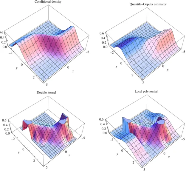
100. For the statistical properties of Frank’s copula, see Nelsen [32] and Genest [33].

Fig. 1shows a plot of the conditional density and its estimates for all

(

x

,

y

)

∈ [−

5

,

5

]×[−

3

,

3

]

. Estimators were computed with fixed, simple rule-of-thumb bandwidth methods based on the Normal reference rule. For the selection ofanof the copula density estimator, we applied Scott’s Rule on the dataFn

(

Xi

)

. We used Epanechnikov kernels forg

ˆ

(

y

)

and the other estimators.

Fig. 1. 3D Plots. From left to right, top to bottom: true density, quantile-copula estimator, double kernel, local polynomial (clipped).

4.3.3. Clipping and estimation in the tails

One major issue of the alternative estimators already mentioned is their numerical instability when the estimated density

ˆ

f

(

x

)

is close to zero. In particular, if the kernel is of compact support, the denominator is zero for thexwhose distance from the closestXiexceeds half the bandwidth times the length of the support, thereby allowing estimation only on a closed subset ofXincluded in

[

minXi

,

maxXi

]

. This is one reason why simulation studies are often performed either with a marginalX density of bounded support and/or with a Gaussian kernel. Note that the problem remains with a Gaussian kernel since the estimated density can become quickly smaller than machine precision.

To avoid numerical problems, the definition of the conditional density estimators have to be modified either by

ˆ

f

(

y

|

x

)

=







ˆ

fXY

(

x

,

y

)

ˆ

fX

(

x

)

iff

ˆ

X

(

x

) >

c

ˆ

a

(

y

)

iff

ˆ

X

(

x

)

=

0 or f

ˆ

(

y

|

x

)

=

ˆ

fXY

(

x

,

y

)

max

{ˆ

f

(

x

),

c

}

,

wherec

>

0 is an arbitrary amount of clipping, anda

ˆ

(

·

)

is an arbitrary density estimator (usually chosen to be zero org

ˆ

(

y

)

). An illustration of these issues appears inFig. 1. The unclipped version of the double kernel estimator is unable to estimate the conditional density for

|

x

|

>

3 roughly, and the clipped version of the local polynomial estimator withc

=

10−5and

ˆ

a

(

y

)

= ˆ

g

(

y

)

gives a wrong estimation in the tails, reflecting the arbitrary choices in the clipping decision. In contrast, the quantile-copula estimator seems to perform well at locationxwhere there is ‘‘no data’’, i.e., in the tails ofX.

Table 1

Mean integrated square error.

Model x y∈ [a,b] QC QC2 DK LP 1 0 [−2, 2] 0.01056 0.00891 0.01459 0.01183 1 3 [−1, 3] 0.03997 0.1091 0.04154 0.7416 2 0 [−2, 2] 0.00735 0.00945 0.00520 0.00664 2 5 [−2, 2] 0.01202 0.0887 0.01748 0.33425 3 0 [0, 1] 0.04385 0.06477 0.10754 0.06398 3 1 [0, 1] 0.0322 0.04102 0.06435 0.04658

4.3.4. Evaluation of the local ISE and MISE

In order to get a closer look at the performance of the estimator, we compared the ISE at a fixedxon a set ofyvalues in an interval

[

a

,

b

]

, viz.

ISE

(

x

)

=

Z

b

a

{ˆ

f

(

y

|

x

)

−

f

(

y

|

x

)

}

2dy

for the different estimators. The ISE

(

x

)

was computed by its approximation on a grid ofN

=

50 values

(

yj

)

, equally spaced of∆on the interval

[

a

,

b

]

. I

(

x

)

=

∆ N

X

j=1

{ˆ

f

(

yj

|

x

)

−

f

(

yj

|

x

)

}

2 (9)

The MISE is then evaluated by averaging the previous quantityI

(

x

)

overm

=

50 Monte Carlo replications of sample size

n

=

100. The simulation was performed on the previous model and on the following ones:

Model 2X

∼

N

(

0

,

1

)

,Y

∼

N

(

0

,

1

)

, andCis the Ali–Mikhail–Haq copula C

(

u

, v)

=

u

v

1

−

θ(

1

−

u

)(

1

−

v)

with

θ

=

0

.

5. For statistical properties of this class of copulas, see Ali et al. [34]. Model 3X

∼

N

(

0

,

1

)

,Y

∼

Exp

(

2

)

,Cis the Gaussian copula with

ρ

=

0

.

75.

In order to avoid biasing the comparisons by a poor choice of smoothing parameters, we used the recommended methods of [31] for the ratio-shaped estimators, together with Gaussian kernels. For the quantile-copula estimator, we selectedhy by the direct plug-in method of Scott [35], andansuch that it contains at least a fixed amount (35%) of the data. For each model, we chose two locations forx, one in the center of theXdistribution, and one away from it. The intervals

[

a

,

b

]

where chosen so that they contains most of the mass of the conditional density at the given locationx. The resulting evaluations of the MISE are summarized inTable 1, where QC stands for the Beta kernel version of the quantile-copula estimator, QC2 for the Gaussian kernel version, DK and LP for double kernel and local polynomial, respectively. The lowest value is highlighted in boldface.

On the whole, the quantile-copula estimator compares favorably to its competitors. At locations where there is ‘‘enough’’ data, the different estimators have a comparable performance, none of them being universally better for all models. We note that the quantile-copula estimator with a symmetric kernel appears to be satisfactory. A good increase of performance is obtained by the quantile-copula estimator with a Beta kernel at ‘‘sparse’’ locations, precisely where its competitors such as the local polynomial may evidence a marked loss of accuracy, as in Model 1,x

=

3, and Model 2,x

=

5.

Acknowledgments

The author is grateful to Prof. Emmanuel Guerre and Christian Genest for their thoughtful comments, which greatly helped in improving the presentation of this article.

Appendix. Auxiliary results

This section assembles the material needed to prove the results of Section3. InAppendix A.1, we recall classical results about the convergence of the Kolmogorov–Smirnov statistic. Next, we provide a brief overview of kernel density estimation and apply these results to the estimatorsg

ˆ

n(Appendix A.2) andcn(Appendix A.3). Approximation lemmas forc

ˆ

nbycnare given inAppendices A.4andA.5.

A.1. Approximation of the pseudo-variables F

(

Xi

)

by their estimates Fn

(

Xi

)

Given a random sampleX1

, . . . ,

Xnfrom a random variableXwith c.d.f.F, the Kolmogorov–Smirnov statistic is defined asDn

= k

Fn

−

F

k

∞. Glivenko and Cantelli, Kolmogorov and Smirnov, Chung and Donsker, among others, have studied its

convergence properties in increasing degree of generality; see [36,16] for recent accounts. For our purpose, we only need to formulate these results in the following rough form:

Lemma A.1. For an i.i.d. sample from a continuous c.d.f. F ,

k

Fn

−

F

k

∞

=

Oa.s.

r

ln lnn n

!

,

(10)

k

Fn

−

F

k

∞

=

OP

1

√

n

.

(11)

BecauseFis unknown, the random variableUi

=

F

(

Xi

)

is not observed. As a consequence ofLemma A.1, one can naturally approximate this variable by the statisticFn

(

Xi

)

. Indeed,

|

F

(

Xi

)

−

Fn

(

Xi

)

| ≤

supx∈R

|

F

(

x

)

−

Fn

(

x

)

| = k

Fn

−

F

k

∞ a.s.

Thus,

|

F

(

Xi

)

−

Fn

(

Xi

)

|

is no more than anOa.s

((

ln lnn

/

n

)

1/2

)

or anOP

(

n−1/2

)

. These rates of approximation are faster than those of statistical estimators of densities, as is shown in the next subsection.

A.2. A reminder on the convergence of kernel density estimators

We recall below some classical results about the convergence of the Parzen–Rosenblatt kernel nonparametric estimator

ˆ

fnof ad-variate densityf. Since its introduction by Rosenblatt [37] and Parzen [38], it has been studied by many authors; see, e.g., Scott [35] or Wand and Jones [39] for details.

It is well known that the bias of the kernel density estimator depends on the degree of smoothness of the underlying density, measured by its number of derivatives or its Lipschitz order. To ensure that the bias is asymptotically negligible, it suffices to assume that the density is continuous; see [38]. To control the rate of convergence of the estimator, it is necessary to make further assumptions. Moreover, for kernel functions with unbounded support, the rate of convergence also depends on the tail behavior of the kernel; see Stute [40]. Therefore, for clarity of exposition and easier notation, we will make the customary assumptions that the density is twice differentiable and that the kernel is of bounded support. Givenxin the interior of supp

(

f

)

,hn

→

0 andnhdn

→ ∞

, we then have the following results:

•

Bias: Ef

ˆ

n

(

x

)

=

f

(

x

)

+

h2_n 2

Z

Rd

X

1≤i,j≤d

∂

2

∂

xi

∂

xj f

(

x

)

zizjK

(

z

)

dz

+

o

(

h2n

).

When the multivariate kernelKis a productK1

× · · · ×

Kdof order-one kernels, the above sum reduces to the diagonal terms. Ef

ˆ

n

(

x

)

=

f

(

x

)

+

h2 n 2

X

1≤i≤d m2

(

Ki

)

∂

2_f

₍

_x

₎

∂

x2_i

+

o

(

h 2 n

).

•

Variance: var

{ˆ

fn

(

x

)

} =

f

(

x

)

nhd n

k

K

k

2₂

+

o

1 nhd n

.

Thus, for a choice of bandwidthhn

'

n−1/(d+4)achieving the optimal trade-off between the bias and variance, one gets the raten−2/(d+4), which is the optimal speed of convergence in the minimax sense in the class of density functions with bounded second derivatives, according to [41].

•

Pointwise asymptotic normality: for anyxsuch thatf

(

x

) >

0,

q

nhd

n

{ˆ

fn

(

x

)

−

Ef

ˆ

n

(

x

)

}

N

(

0

,

f

(

x

)

k

K

k

22

).

If, in additionnhd+4

n

→

0, the bandwidth is small enough to make the bias negligible, so that one gets

q

nhd

•

Pointwise almost sure convergence: if in additionnhd_n

/(

ln lnn

)

→ ∞

(see [42]), we have

ˆ

fn

(

x

)

−

Ef

ˆ

n

(

x

)

=

Oa.s.

s

ln lnn nhd n

!

.

For a choice of bandwidthhn

' {

(

ln lnn

)/

n

}

1/(d+4), we get the rate of convergence

{

(

ln lnn

)/

n

}

2/(d+4):

ˆ

fn

(

x

)

−

f

(

x

)

=

Oa.s.

ln lnn n

2/(d+4)

!

.

A.3. Convergence ofg

ˆ

nand cn

(

u

, v)

The above results can be summarized as follows in the special cased

=

1, which pertains to the estimatorg

ˆ

nof the densitygofY:

Lemma A.2.With the previous assumptions, for a point y in the interior of the support of g, we have:

•

for hn

'

n−1/5,

g

ˆ

_n

(

y

)

−

g

(

y

)

=

O_p

(

n−2/5

)

;

•

for hn

=

o

(

n−1/5

)

,

√

nhn

{ ˆ

gn

(

y

)

−

g

(

y

)

}

N 0

,

g

(

y

)

k

K0

k

22

;

•

for hn

'

(

ln lnn

/

n

)

1/5,g

ˆ

n

(

y

)

−

g

(

y

)

=

Oa.s.

ln lnn n

2/5

.

As mentioned before, the assumption thatFandGare differentiable and strictly increasing entails thatcis the density of the transformed variables

(

U

,

V

)

=

(

F

(

X

),

G

(

Y

))

. Therefore, sincecn

(

u

, v)

is simply the kernel density estimator of the bivariate densityc

(

u

, v)

of the pseudo-variables

(

U

,

V

)

, one directly draws its convergence properties by applying the results of the preceding subsection withd

=

2.

Lemma A.3.For every

(

u

, v)

∈

(

0

,

1

)

2, similar results of those of LemmaA.2hold for

ˆ

cn, with a choice of bandwidth of an

'

n−1/6or an

'

(

n

/

ln lnn

)

−1/6, with a rate of convergence of n−1/3and

(

ln lnn

/

n

)

1/3respectively.

A.4. An approximation lemma ofc

ˆ

n

(

u

, v)

by cn

(

u

, v)

The following lemma gives the rate of approximation of the kernel copula density estimatorc

ˆ

n

(

u

, v)

computed on the data

(

Fn

(

Xi

),

Gn

(

Yi

))

by its analoguecn

(

u

, v)

computed on the pseudo-data

(

Ui

,

Vi

)

=

(

F

(

Xi

),

G

(

Yi

))

. A similar result, but with a different proof, was obtained by Fermanian [20]; see his Theorem 1.

Lemma A.4.Let

(

u

, v)

∈

(

0

,

1

)

2_{. If the kernel K}

₍

_u

_{, v)}

₌

_K

1

(

u

)

K2

(v)

is twice differentiable with bounded second derivatives,

then

|ˆ

cn

(

u

, v)

−

cn

(

u

, v)

| =

OP n−1/2

+

1 na4 n

+

√

ln lnn na3 n

!

,

|ˆ

cn

(

u

, v)

−

cn

(

u

, v)

| =

Oa.s.

ln lnn n

1/2

+

(

lnnln lnn

)

1/2 na3 n

+

ln lnn na4 n

!

.

Proof. Let

k · k

denote a vector norm. Set

∆

= ˆ

cn

(

u

, v)

−

cn

(

u

, v)

=

n

X

i=1 ∆i,n

(

u

, v)/(

na2n

)

with ∆i,n

(

u

, v)

=

K

u

−

Fn

(

Xi

)

an

,

v

−

Gn

(

Yi

)

an

−

K

u

−

F

(

Xi

)

an

,

v

−

G

(

Yi

)

an

and define Zi,n

=

F

(

Xi

)

−

Fn

(

Xi

)

G

(

Yi

)

−

Gn

(

Yi

)

.