Modelling UK House Prices with Structural Breaks and Conditional
Variance Analysis
Kyriaki Begiazi
1and Paraskevi Katsiampa
2Abstract
This paper differs from previous research by examining the existence of structural breaks in
the UK regional house prices as well as in the prices of the different property types (flats, terraced,
detached and semi-detached houses) in the UK as a whole, motivated by the uncertainty in the UK
housing market and various financial events that may lead to structural changes within the housing
market. Our paper enhances the conventional unit root tests by allowing for structural breaks, while
including structural break tests strengthens our analysis. Our empirical results support the existence of
structural breaks in the mean equation in seven out of thirteen regions of the UK as well as in three out
of four property types, and in the variance equation in six regions and three property types. In addition,
using a multivariate GARCH approach we examine both the behaviour of variances and covariances of
the house price returns over time. Our results have significant implications for appropriate economic
policy selection and investment management.
Keywords
UK regions, House prices,
Structural break, Volatility, MGARCH, BEKK
JEL Classifications:
C22, C32, G1, R15
1Department of Accounting, Finance and Economics, Oxford Brookes University, Oxford, OX3 0BP, UK 2 Sheffield Business School, Sheffield Hallam University, Sheffield, S1 1WB, UK
Kyriaki Begiazi
Paraskevi Katsiampa
Acknowledgements
The authors gratefully acknowledge the valuable comments and suggestions of two anonymous
referees.
Introduction
Recently a trend of long-run growth has been observed in house prices across the world.As housing markets play an important role in the economy, analysing their behaviour across time is important in order to understand them and improve our investment and risk strategies. Interestingly, house prices share some properties with financial time series (see, e.g., Dolde and Tirtiroglu 1997; Campbell et al. 2009; Miles 2011a; Lin and Fuerst 2014), and hence appropriate modelling of housing markets, and house prices in particular, is therefore of high importance (Antonakakis et al. 2015).
Examining housing markets effectively is important for suitable economic policy selection as well as risk management, not only at national but also at regional level. Risk management is based on volatility and recent financial events have increased the market uncertainty (e.g., financial crisis, UK referendum). Previous research has revealed that some UK areas exhibit conditional variances (see, e.g., Willcocks 2010). As linear models are unable to explain features such as leptokurtosis, volatility clustering and leverage effects, recently there has been an increased academic interest in the modelling of house prices by using the class of Generalised Autoregressive Conditional Heteroscedasticity (GARCH) models. Previous studies have employed different univariate GARCH-type models for house price volatility. However, the housing market is influenced by local characteristics that could lead to dynamic interlinkages (Miao et al. 2011), and a limitation of the univariate volatility models is that they model only individual conditional variances. Even though multivariate GARCH extensions could help us investigate a joint approach to modelling house price volatilities, there is rather limited literature on multivariate studies of house prices across different markets.
Furthermore, although there are many studies on the UK housing market, there is limited research on the different property types in the UK. These include flats, terraced houses, semi-detached and detached houses. It is important to analyse each property type separately, as various forms of housing are used for different purposes and attract different types of investors (Morley and Thomas 2016).
Finally, real estate markets are often subject to large shocks that could create a structural break. In the UK in particular there is strong evidence of house price crashes. For instance, in 2007 house prices in Northern Ireland peaked at the top of the bubble and then started falling until 2010. Although it is of paramount importance to test for structural breaks if the period under study covers unstable periods, as not considering the structural breaks could lead to incorrect conclusions (Chien 2008), while breaks in the variance could look as ARCH effects (Diebold 1986) and empirical verification of theories can depend on structural breaks (Lee et al. 2006), most of the earlier studies did not test for structural breaks before modelling conditional volatilities. If ARCH effects are found for the whole period, but not for the sub-periods, that can be an indication of a break in the unconditional variance and not ARCH effects.
Consequently, we aim to contribute to the literature by analysing the UK, both in regional level as well as by property type, by including structural break tests in both the mean and variance equations, in order to identify specific breakpoints which could help us correlate them with specific events (e.g., financial crisis, policies, UK referendum, etc.). Upon identification of breakpoints, each region and property type is tested for ARCH effects, and for those series exhibiting volatility clustering but no structural break in the mean or variance, their volatility is analysed on a multivariate basis in order to investigate whether there exist any interdependencies, as multivariate GARCH (MGARCH) models could examine the movements of the covariances among different regions and property types.
Manuscript (BLINDED: WITHOUT author information) Click here to view linked References
1 2 3 4 5 6 7 8 9 10 11 12 13 14 15 16 17 18 19 20 21 22 23 24 25 26 27 28 29 30 31 32 33 34 35 36 37 38 39 40 41 42 43 44 45 46 47 48 49 50 51 52 53 54 55 56 57 58 59 60 61
The remainder of the paper is organised as follows: The next section reviews the relevant literature, followed by a description of the data and methodology used in this study. The fourth section discusses the empirical findings. Finally, the conclusions drawn and the implications for policy making are presented in the last section.
Literature review
In recent years there has been heightened academic interest in house price dynamics. An increased number of studies has examined house price volatility by employing theclass of GARCH models. Previous studies have employed various univariate GARCH-type models for house price volatility, such as GARCH and GARCH-in-Mean (GARCH-M) (e.g., Dolde and Tirtiroglu 1997; Stevenson et al. 2007; Hossain and Latif 2009), Exponential GARCH (EGARCH) and Exponential GARCH-in-Mean (EGARCH-M) (e.g., Lee 2009; Willcocks 2010; Lin and Fuerst 2014; Morley and Thomas 2011, 2016), Component GARCH (CGARCH) and Component GARCH-in-Mean (CGARCH-M) (Miles 2011a; Lee and Reed 2013; Karoglou et al. 2013).
However, most of the literature has focused on analysing house price volatility by using univariate GARCH-type models and, even though a large number of studies have used asset interlinkages to analyse volatility relationships (Miao et al. 2011),there is rather limited literature on multivariate studies of house prices across different markets and on volatility linkages in real estate markets, which often exist. In general, volatility linkages can occur as a result of information that changes expectations and demand or cross-market hedging (Miao et al. 2011).Earlier studies using multivariate models for house prices include the Vector Autoregressive (VAR) (Miller and Peng 2006; Hossain and Latif 2009) and the Vector Error Correction model (Damianov and Escobari 2016), whilemultivariate GARCH (MGARCH)-type models used in previous studies of volatility spillovers in real estate markets include the BEKK-MGARCH (Willcocks 2010; Miao et al. 2011) and the Dynamic Conditional Correlation (DCC) model (Antonakakis et al. 2015). Moreover, Begiazi et al. (2016) used DCC and BEKK-MGARCH model to test volatility spillover among global Real Estate Investment Trusts (REITs) and found that the REIT market is becoming increasingly globalised.
Furthermore, even though recently there has been an increased interest in studies of multivariate analyses of house prices in the US (Miao et al. 2011; Antonakakis et al. 2015; Damianov and Escobari 2016), and although the dynamics of the UK housing prices have been extensively studied in the literature over the last decade, with studies of regional house prices in the UK including those of Stevenson et al. (2007), Tsai et al. (2010), Willcocks (2010), Miles (2011b), and Morley and Thomas (2011, 2016), multivariate analyses of UK house prices are very limited. To the best of the authors' knowledge, only Willcocks (2010) considered studying the UK house prices in a multivariate basis. Nevertheless, Willcocks (2010) did not consider analysing the different property types (flats, terraced houses, semi-detached and detached houses). In fact, there is very limited research on the different property types in the UK too. Again to the best of the authors' knowledge, only Morley and Thomas (2016) considered examining each property type individually, but not on a multivariate basis.
Another crucial aspect to consider is the stationarity and stability of house prices. Meen (1999) and Peterson et al. (2002), under standard unit-root tests, found that the UK house prices follow a random walk process. However, real estate markets are often subject to large shocks that could create structural breaks and, according to Lee et al. (2006), structural breaks are important in modelling and forecasting. Moreover, Diebold (1986) showed that breaks in the variance could look as ARCH effects. In addition, Perron (1989, 1997) proposed to
1 2 3 4 5 6 7 8 9 10 11 12 13 14 15 16 17 18 19 20 21 22 23 24 25 26 27 28 29 30 31 32 33 34 35 36 37 38 39 40 41 42 43 44 45 46 47 48 49 50 51 52 53 54 55 56 57 58 59 60 61
include structural breaks in the ADF unit root test, while, according to Rapach and Straus (2008), a structural break analysis could improve the accuracy of volatility forecast.
Therefore, it is of high importance to explore the model stability before looking for ARCH effects. However, even though the analysis of extreme events has become very popular nowadays (Hansen 2001), a lot of empirical papers have not tested for structural breaks prior to modelling conditional volatilities and the conventional unit root test may be misleading in the presence of breakpoints. Once again to the best of the authors' knowledge, with regards to real estate markets, only Chien (2010) and Canarella et al. (2012) differed their studies by allowing for breakpoints in the Taiwan and US housing markets, respectively, while none of the aforementioned studies on the UK house price dynamics tested for structural breaks prior to proceeding with modelling conditional variances.
As it has been previously shown that UK regions exhibit conditional volatilities (see, e.g., Willcocks 2010; Morley and Thomas 2016), this paper aims to extend the literature by employing a multivariate GARCH - diagonal BEKK model to examine house price volatility in the regions of the UK as well as in the property types within the whole UK, for those series exhibiting ARCH effects, but most importantly adds to the existing literature on the UK house prices by first testing for structural breaks in both the mean and variance equations of each time series in order to strengthen our analysis and validate our results.
Data and Methodology
This paper uses UK regional quarterly house price data from Nationwide’s House Price Index from the fourth quarter of 1973 to the first quarter of 2017, giving a total of 174 observations. Furthermore, we use aggregate UK quarterly series by property type, from the first quarter of 1991 to the first quarter 2017. All the data are publicly available online at http://www.nationwide.co.uk/about/house-price-index/download-data#tab:Downloaddata.
The data are converted to natural logarithms, and then we define the housing returns for each region and property type as
𝑅𝑖𝑡= (𝑙𝑛𝑦𝑖𝑡− 𝑙𝑛𝑦𝑖𝑡−1) (1) where 𝑅𝑖𝑡 is the logarithmic house price index return in quarter
t
for UK regioni
or house property typei
, and𝑦𝑖𝑡 is the house price index in quarter
t
for UK regioni
or house property typei
.First of all, using the Augmented Dickey-Fuller (ADF) test, we check whether our logarithmic house price indices as well as our return series have a unit root or not. According to Perron (1989), we have to identify any structural change when we test for unit roots, though. Standard unit root tests could be biased toward a false unit root null. Therefore, we also run modified Dickey-Fuller tests with breakpoints for intercept and trend. Our analysis follows the work of Perron (1989), Perron and Vogelsang (1992), Banerjee et al. (1992) and Vogelsang and Perron (1998). For each possible break date (the start of the new regime), the optimal number of lags is chosen using the Schwarz criterion, and the Dickey-Fuller t-statistic is computed. We test two different models that both assume an innovation outlier break, as follows
non-trending data with intercept break:
𝑅𝑡= 𝜇 + 𝜃𝐷𝑈𝑡(𝑇𝑏) + 𝜔𝐷𝑡(𝑇𝑏) + 𝑎𝑅𝑡−1+ ∑𝑘𝑖=1𝑐𝑖Δ𝑅𝑡−1+ 𝜀𝑡 (2) 1 2 3 4 5 6 7 8 9 10 11 12 13 14 15 16 17 18 19 20 21 22 23 24 25 26 27 28 29 30 31 32 33 34 35 36 37 38 39 40 41 42 43 44 45 46 47 48 49 50 51 52 53 54 55 56 57 58 59 60 61
trending data with intercept and trend break:
𝑅𝑡= 𝜇 + 𝛽𝑡+ 𝜃𝐷𝑈𝑡(𝑇𝑏) + 𝛾𝐷𝑡(𝑇𝑏) + 𝜔𝐷𝑡(𝑇𝑏) + 𝑎𝑅𝑡−1+ ∑𝑘𝑖=1𝑐𝑖Δ𝑅𝑡−1+ 𝜀𝑡 (3) where 𝜀𝑡are i.i.d. innovations, k represents the lag order, 𝐷𝑈𝑡(𝑇𝑏) is the intercept break variable that takes the value 0 prior to and 1 after the break, 𝐷𝑡(𝑇𝑏) is the one-time break dummy variable which takes the value of 1 only on the break date and 0 otherwise. Both models include the intercept break (θ) and break dummy coefficients (ω), while 𝛽 and γ are the trend and trend break coefficients, respectively, included only in the second model. Note that the full impact of the break variables occurs immediately.
Then, we continue by conducting breakpoint tests for one or more structural breakpoints for an Autoregressive (AR) mean equation process with a constant, according to Bai and Perron (2003), fitted to our return series, choosing the lag order based on the significance of the estimated parameters. Similarly, Göktaş and Dişbudak (2014) used an AR model to examine whether there is a structural break in Turkey’s inflation series. More specifically, we test the implicit assumption that the parameters of the Autoregressive (AR) model are constant for the entire sample using parameter stability tests. Chow's breakpoint and predictive failure tests are satisfactory only if we know the date of the structural break for each time series (Brooks 2014). Quandt (1960) developed a modified version of the Chow test that allows the estimation with unknown break dates. The test computes the usual Chow F-statistic constantly with different break dates and chooses the break date with the highest F-statistic value. Then, Andrews (1993) extended the methodology and provided methods to calculate appropriate p-values. More recently, Bai and Perron (1998, 2003) extended the Quandt-Andrews test by allowing for multiple unknown breakpoints, which is the structural break test we use in our analysis. However, we also need to test for potential breakpoints in the variance. Consequently, similar to Göktaş and Dişbudak (2014), the squared residuals of the AR models are regressed on a constant, and Bai-Perron tests are then reperformed.
Once any structural break is identified, following Miller and Peng (2006) and Willcocks (2010), each region or property type without any breakpoint in the mean or variance equation is modelled by an ARMA (p,q) process. The general ARMA (p,q) is shown below:
𝑅𝑡,𝑖= 𝜇 + 𝜑1𝑅𝑡−1+ ⋯ + 𝜑𝑝Rt−p,i+ 𝜀𝑡,𝑖+ 𝜃1𝜀𝑡−1,𝑖+ ⋯ 𝜃𝑞𝜀𝑡−𝑞,𝑖 (4) We select the appropriate regional lag structure, by using information criteria, on the basis that there is heterogeneity across different areas. For a justification of why there could be a lack of homogeneity in housing markets across regions, see, e.g., Miller and Peng (2006).
The residuals from these models are then tested for the existence of ARCH effects. For those regions or property types without any structural breaks in the mean and variance equations, but which exhibit volatility clustering, multivariate GARCH modelling is employed in order to model the conditional variances and examine the linkages among the different regions and property types. A limitation of univariate volatility models is that the fitted conditional variance of each series is entirely independent of all others. However, covariances can provide a lot of useful information. Multivariate GARCH models enable us to estimate the conditional volatilities of the variables simultaneously. The main reason why we have selected a multivariate model is the fact that shocks which increase uncertainty in one housing market could also increase the uncertainty in another housing market,
1 2 3 4 5 6 7 8 9 10 11 12 13 14 15 16 17 18 19 20 21 22 23 24 25 26 27 28 29 30 31 32 33 34 35 36 37 38 39 40 41 42 43 44 45 46 47 48 49 50 51 52 53 54 55 56 57 58 59 60 61
and, hence, employing univariate models to study the conditional variance of each market separately is not appropriate for examining interlinkages of different housing markets.
In order to examine the co-movements among different housing market returns, we employ the multivariate GARCH-BEKK model of Engle and Kroner (1995), with the restriction that A and B matrices are diagonal. The model known as diagonal BEKK has the following form:
𝐻𝑡= 𝐶𝐶′ + 𝛢𝜀𝑡−1𝜀𝑡−1′𝐴′ + 𝛣𝛨𝑡−1𝐵′ (5) where 𝐻𝑡 is a N x N conditional variance-covariance matrix, C is a an N(N+1)/2 matrix of the intercepts, while A and B are both diagonal matrices of order N. The elements of the variance-covariance matrix, 𝐻𝑡, depend only on past values of itself and past values of squared errors. Matrix A measures the effects of past squared errors (news) on current conditional variances (ARCH effects) and matrix B explains how past conditional variances (volatility persistence) affect the current levels of conditional variances (GARCH effects).
The reason why we have chosen the diagonal BEKK, instead of, e.g., the full BEKK, is due to the “curse of dimensionality”. The number of parameters in a full BEKK model can be as much as 3N(N+1)/2, where N is the number of time series included in the model and the estimation can become problematic and less reliable (Chang and McAleer 2017). In fact, Chang and McAleer (2017) further showed that estimation of the full BEKK could have some problems even with only five assets, while that is not an issue in the case of the diagonal BEKK model.
Another benefit in our analysis of employing the multivariate GARCH-diagonal BEKK model is that we can examine how the variances and covariances move over time. It can also be noted that the diagonal BEKK model is similar to the diagonal VECH model of Bollerslev et al. (1988), with order one coefficient matrices, but, in contrast to the diagonal VECH, the diagonal BEKKmodel ensures positive conditional variances.
Finally, the conditional variance of region or property type i, ℎ𝑖𝑡, i = 1, …., N, can also be expressed as:
ℎ𝑖𝑡= 𝑐𝑖𝑖+ 𝑎𝑖𝑖2𝜀𝑖𝑡−12+ 𝛽𝑖𝑖2ℎ𝑖𝑡−1 (6) while the conditional covariance between two regions or property types i and j, ℎ𝑖𝑗𝑡, where i, j = 1, …., N,
i
j
, can be expressed as:ℎ𝑖𝑗𝑡 = 𝑐𝑖𝑗+ 𝑎𝑖𝑖𝑎𝑗𝑗𝜀𝑖𝑡−1𝜀𝑗𝑡−1+ 𝛽𝑖𝑖𝛽𝑗𝑗ℎ𝑖𝑗𝑡−1 (7)
Empirical Findings
UK house prices by region
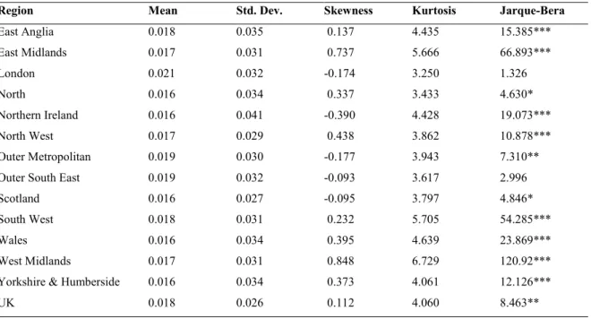
Table 1 presents basic descriptive statistics of the regional house price returns. The quarterly mean returns range from 1.6% (Yorkshire and Humberside) to 2.1% (London), while the standard deviation ranges from 2.7% (Scotland) to 4.1% (Northern Ireland). The UK as a whole reports 1.8% mean return and 2.6% standard deviation. The results of the Jarque-Bera test (Jarque and Bera 1980) show that only London and Outer South East do not reject the normal distribution hypothesis at any significance level. The lack of symmetry is further highlighted by the statistics of skewness and kurtosis. Our data tend to exhibit high kurtosis and have heavier tails than the normal
1 2 3 4 5 6 7 8 9 10 11 12 13 14 15 16 17 18 19 20 21 22 23 24 25 26 27 28 29 30 31 32 33 34 35 36 37 38 39 40 41 42 43 44 45 46 47 48 49 50 51 52 53 54 55 56 57 58 59 60 61
distribution. It can also be noticed that all regions, apart from London, Northern Ireland, Outer Metropolitan, Outer South East and Scotland, report positive skewness.
Table 1 Descriptive statistics of regional house price returns
Region Mean Std. Dev. Skewness Kurtosis Jarque-Bera
East Anglia 0.018 0.035 0.137 4.435 15.385*** East Midlands 0.017 0.031 0.737 5.666 66.893*** London 0.021 0.032 -0.174 3.250 1.326 North 0.016 0.034 0.337 3.433 4.630* Northern Ireland 0.016 0.041 -0.390 4.428 19.073*** North West 0.017 0.029 0.438 3.862 10.878*** Outer Metropolitan 0.019 0.030 -0.177 3.943 7.310** Outer South East 0.019 0.032 -0.093 3.617 2.996
Scotland 0.016 0.027 -0.095 3.797 4.846*
South West 0.018 0.031 0.232 5.705 54.285***
Wales 0.016 0.034 0.395 4.639 23.869***
West Midlands 0.017 0.031 0.848 6.729 120.92***
Yorkshire & Humberside 0.016 0.034 0.373 4.061 12.126***
UK 0.018 0.026 0.112 4.060 8.463**
Significant at *10%, **5%, ***1%
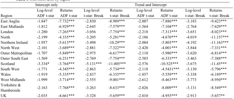
Since breaks could look as ARCH effects when the whole sample is used (Diebold 1986), modelling the conditional variance by a GARCH process will be the wrong thing to do without testing for structural breaks first. As a result, standard unit root tests, such as ADF tests (Dickey and Fuller 1979), were implemented in order to examine the stationarity of the regional logarithmic house prices and house price returns, along with breakpoint unit root tests, as structural breaks could distract the ADF test results. Our unit root tests minimise endogenously the Dickey-Fuller t-statistic in order to select a breakpoint, and select a lag length using the Schwarz criterion. Table 6 (Appendix I) summarises the results of the ADF tests with and without a breakpoint on our time series (in log-levels and returns), including either only an intercept, or both an intercept and trend, in the test equation. The log-levels reported unit roots but, when we examined the return series, the tests rejected the null hypothesis of the unit root suggesting that all our return series are stationary. The only exception is Scotland which is also stationary in log-levels when including an intercept break.
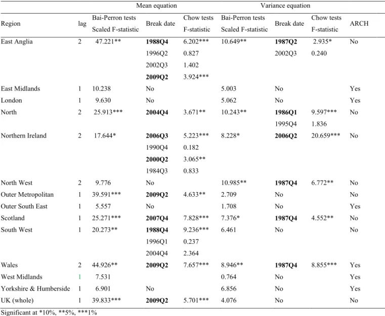
We continued our analysis by conducting tests for structural breaks in the Autoregressive (AR) mean equation process with a constant, in accordance with Bai and Perron (2003), fitted to our regional house price index returns, choosing the lag order based on the significance of the estimated parameters. We performed sequential testing of
l+1 versus l breaks based on Bai (1997) and Bai and Perron (1998) and allowed for error heterogeneity, using the Bai and Perron (2003) critical values.For the series exhibiting structural breaks as obtained from the sequential procedure, we also used Chow's breakpoint test in order to verify whether a suggested breakpoint date is indeed a breakpoint. The results of these multiple breakpoint tests together with Chow's breakpoint tests are reported in Table 2. 1 2 3 4 5 6 7 8 9 10 11 12 13 14 15 16 17 18 19 20 21 22 23 24 25 26 27 28 29 30 31 32 33 34 35 36 37 38 39 40 41 42 43 44 45 46 47 48 49 50 51 52 53 54 55 56 57 58 59 60 61
Table 2 Multiple Bai-Perron breakpoint tests by region
Mean equation Variance equation Region lag Bai-Perron tests
Scaled F-statistic Break date
Chow tests F-statistic
Bai-Perron tests
Scaled F-statistic Break date
Chow tests F-statistic ARCH East Anglia 2 47.221** 1988Q4 6.202*** 10.649** 1987Q2 2.935* No 1996Q2 0.827 2002Q3 0.240 2002Q3 1.402 2009Q2 3.924***
East Midlands 1 10.238 No 5.003 No Yes
London 1 9.630 No 5.062 No Yes North 2 25.913*** 2004Q4 3.671** 10.243** 1986Q1 9.597*** No 1995Q4 1.836 Northern Ireland 2 17.644* 2006Q3 5.223*** 8.228* 2006Q2 20.659*** No 1990Q4 0.182 2000Q2 3.065** 1984Q3 0.833 North West 2 9.776 No 10.985** 1987Q4 6.772** No Outer Metropolitan 1 39.591*** 2009Q2 4.633** 2.709 No No
Outer South East 1 5.557 No 1.708 No Yes
Scotland 1 25.271*** 2007Q4 7.828*** 7.376* 1987Q4 4.552** No
South West 1 20.273** 1988Q4 9.236*** 6.461 No No
1996Q1 0.237 2004Q4 2.364
Wales 2 44.926** 2009Q2 7.657*** 8.946** 1987Q4 8.855*** Yes
West Midlands 1 7.531 0.764 No Yes
Yorkshire & Humberside 1 6.901 No 6.856 No Yes
UK (whole) 1 39.833*** 2009Q2 5.701*** 4.076 No No
Significant at *10%, **5%, ***1%
The results indicate that six (East Midlands, London, North West, Outer South East, West Midlands, Yorkshire and Humberside) out of thirteen regions exhibit no structural break in the mean equation. Interestingly, East Anglia has two structural breaks during the period under examination, while the remaining regions (North, Northern Ireland, Outer Metropolitan, Scotland, South West, Wales, as well as the UK as a whole) have one breakpoint each. More specifically, the structural break dates identified include the fourth quarter of 1988 for East Anglia and South West. This date could be linked to the late 1980s housing boom followed by the early 1990s crash. Other structural break dates identified and verified by Chows' test at 1% significance level include the fourth quarter of 2004 for North, the third quarter of 2006 for Northern Ireland and the fourth quarter of 2007 for Scotland. The breakpoints in Northern Ireland and Scotland in particular seem to be related to the Irish property bubble (prices in Ireland peaked in 2006) and the recent financial crisis, respectively, while the breakpoint identified in North (fourth quarter of 2004) could be related to the Bank of England's interest rate increase which occurred in the third quarter of 2004. By most measures, housing prices started declining in June 2004, as U.K. buyers - who typically finance their assets purchased with monthly adjustable-rate loans - did eventually take notice of the Bank of England's increased rates. It is also worth mentioning that the region of North is one of the
1 2 3 4 5 6 7 8 9 10 11 12 13 14 15 16 17 18 19 20 21 22 23 24 25 26 27 28 29 30 31 32 33 34 35 36 37 38 39 40 41 42 43 44 45 46 47 48 49 50 51 52 53 54 55 56 57 58 59 60 61
regions with the lowest prices in England. Finally, the second quarter of 2009 seems to be a break date for East Anglia, Outer Metropolitan, Wales, and the UK as a whole, and could be related to the house price recovery of the 2007-2008 financial crisis in early 2009.
We also tested for ARCH effects and found that six out of thirteen regions, namely East Midlands, London, Outer South East, Wales, West Midlands, and Yorkshire and Humberside, exhibit volatility clustering. However, as breaks in the variance could look as ARCH effects (Diebold 1986), we also tested for breakpoints in the variance of each region. Following Göktaş and Dişbudak (2014), the squared residuals of the least squares estimation of the above AR models, taking the identified breakpoints into account as appropriate, were regressed on a constant, and Bai-Perron tests were then reperformed. Again for any breakpoint identified by the Bai-Perron tests, we also performed Chow's breakpoint tests in order to verify whether a suggested breakpoint date is indeed a structural break. These results can also be found in Table 2.
According to the results, six regions (East Anglia, North, Northern Ireland, North West, Scotland and Wales) exhibit structural breaks in the variance, five of which (East Anglia, North, Northern Ireland, Scotland and Wales) also exhibit structural breaks in the mean equation. However, with Northern Ireland being the only exception (exhibiting a breakpoint in the second quarter of 2006), the structural break dates identified in the variance of these regions are different to those identified in the mean equation, and include the first quarter of 1986 (North), the second quarter of 1987 (East Anglia), as well as the fourth quarter of 1987 (North West, Scotland and Wales). In the 1980s there were important policy changes in the UK real estate market, such as the deregulation of the UK building societies. More specifically, in 1986, legislation was passed to allow building societies to diversify, offer loans and demutualise as long as they could gain sufficient support from member owners, and the aforementioned breakpoints in the late 1980s could be linked to that. These measures led to increased home ownership and mortgage financing. In fact, according to Cameron et al. (2006), real estate purchased was increased before the end of the tax relief in 1988. In addition, the breakpoint identified in the fourth quarter of 1987 for North West, Scotland and Wales could also be linked with the stock market crash which took place in October 1987, also known as Black Monday. Another interesting finding is that, apart from Wales, which has a structural break in both the mean and variance equations, no structural break has been identified in either the mean or variance equation for any of the other five regions exhibiting volatility clustering (East Midlands, London, Outer South East, West Midlands, and Yorkshire and Humberside), and hence the apparent ARCH effects in Wales could be due to the structural break in variance.
Next, we proceeded with fitting ARMA models to the house price returns of the five regions with ARCH effects but without any structural break in the mean or variance equation (East Midlands, London, Outer South East, West Midlands, Yorkshire and Humberside). Information criteria have been used to select the most appropriate model. We have found that different ARMA lag orders are present, a finding which is in accordance with Miller and Peng (2006) and Willcocks (2010), who highlight that the housing market is heterogeneous and buyers form their expectations based on the local experience. These results together with the results obtained from the ARCH tests performed are summarised in Table 7 (Appendix I). The result of non-constant conditional variances for these regions is overall in accordance with Willcocks (2010) who found evidence of volatility clustering for East Midlands, Outer South East, West Midlands and Yorkshire and Humberside. Our results indicate that London also exhibits ARCH effects. On the other hand, Willcocks (2010) found ARCH effects for
1 2 3 4 5 6 7 8 9 10 11 12 13 14 15 16 17 18 19 20 21 22 23 24 25 26 27 28 29 30 31 32 33 34 35 36 37 38 39 40 41 42 43 44 45 46 47 48 49 50 51 52 53 54 55 56 57 58 59 60 61
Northern Ireland, South West and Wales as well. However, we have found that all of these three regions have structural breaks.
Therefore, we proceeded by using the five regions with time-varying variances and without structural breaks in either the mean or variance equation to create a multivariate diagonal-BEKK model. As we have five assets, estimation of other multivariate GARCH models can become rather infeasible, while our choice of the diagonal BEKK model seems to be appropriate with a total of twenty five parameters to be estimated. The estimation results of the conditional variance coefficients can be found in Table 3. As can be easily seen from the results, all the parameter estimates are statistically significant apart from the past conditional volatility coefficients, β's, for London and West Midlands. The model equations indicate that current conditional variance should be positively affected by past squared errors and past conditional volatility. Similarly, current covariance should be positively affected by the past covariance term and cross product of error terms. However, for London and West Midlands current conditional variances seem to be positively affected only by past squared errors due to the fact that the volatility coefficient beta is statistically insignificant for both regions. As a result, in the case of London and West Midlands past conditional variances do not have a significant effect on the current conditional variances.
Table 3 Diagonal BEKK Variance Coefficients
i-j c 𝑎𝑖𝑖 𝑎𝑗𝑗 𝛽𝑖𝑖 𝛽𝑗𝑗 EM-L 0.000*** 0.414*** 0.414*** 0.764*** 0.309 EM-OSE 0.000*** 0.414*** 0.372*** 0.764*** 0.508*** EM-WM 0.000*** 0.414*** 0.422*** 0.764*** 0.182 EM-YH 0.000*** 0.414*** 0.458*** 0.764*** 0.622*** L-OSE 0.001*** 0.379*** 0.372*** 0.309 0.508*** L-WM 0.000*** 0.379*** 0.422*** 0.309 0.182 L-YH 0.000*** 0.379*** 0.458*** 0.309 0.622*** OSE-WM 0.000*** 0.372*** 0.422*** 0.508*** 0.182 OSE-YH 0.000*** 0.372*** 0.458*** 0.508*** 0.622*** WM-YH 0.000*** 0.4218*** 0.4577*** 0.182 0.622***
Covariance specification: ℎ𝑖𝑗𝑡= 𝑐𝑖𝑗+ 𝑎𝑖𝑖𝑎𝑗𝑗𝜀𝑖𝑡−1𝜀𝑗𝑡−1+ 𝛽𝑖𝑖𝛽𝑗𝑗ℎ𝑖𝑗𝑡−1. Significant at ***1%.
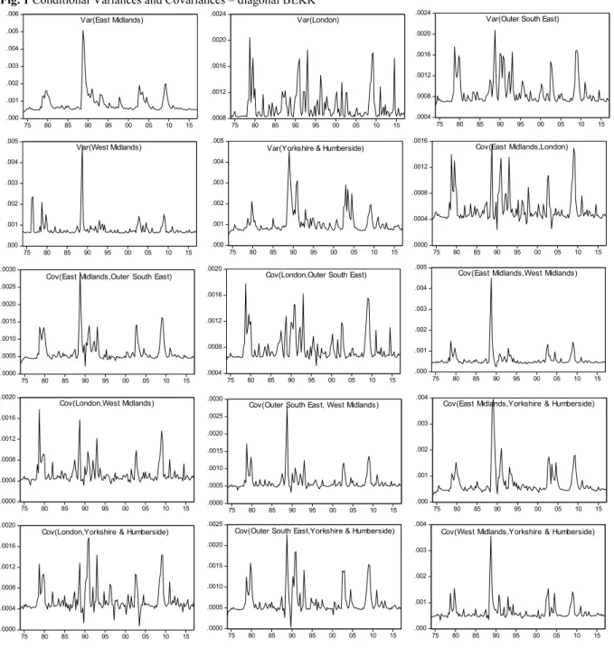
The graphs of the conditional variances and covariances are presented in Figure 1 (Appendix II). The covariance between different regions measures the association between them. According to these plots, the covariances between London and other regions are more volatile than the covariances between the different regions themselves in the UK. This could be explained by the fact that London’s variance appears as the most volatile and that seems to affect the corresponding covariances. However, a covariance could also pick some of the hedging activity in housing markets (Han 2013). As housing in London could be used as a hedge for home owners in the regions, these covariance results could be picking this effect up. Regional hedging is present when households use their current home to hedge against future housing consumption risk. Ortalo-Magne and Rady (2002) also highlighted the importance of the covariance between the current and future homes under consideration because investing in a home is a good hedge against fluctuations in the future home. It is also worth mentioning that house prices in London are interestingly high. According to Hilber and Vermeulen (2016), high prices are driven by strong demand for housing in conjunction with physical constraints. Thus, demand shocks
1 2 3 4 5 6 7 8 9 10 11 12 13 14 15 16 17 18 19 20 21 22 23 24 25 26 27 28 29 30 31 32 33 34 35 36 37 38 39 40 41 42 43 44 45 46 47 48 49 50 51 52 53 54 55 56 57 58 59 60 61
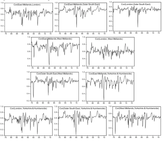
could have a stronger impact on house prices in places with limited developable land supply. The UK has inelastic supply (Malpezzi and Maclennan 2001), while London’s housing market, in particular, is fast growing, a characteristic that could enhance cross-market differences. Furthermore, high rates of returns can lead to high risk exposure. However, the variations of hedging, supply constraints and urban market growth could lead to an inverse risk-return relationship (Han 2013). Finally, a plot of the conditional correlations (Figure 2, Appendix II) indicates that the correlation seems to be time varying, which is a general characteristic of the model.
UK house prices by property type
This study also analyses the house price dynamics of the different property types, namely flats, terraced houses, semi-detached and detached houses. The following analysis focuses on the four property types in the UK as a whole. Table 4 illustrates descriptive statistics of the house price returns by property type. According to the results, the mean returns vary from 1.2% (detached) to 1.4% (flats and terraced), while the standard deviation ranges from 2.3% (detached) to 3.6% (flats). Moreover, although the normal distribution hypothesis cannot be rejected for any of the four property types according to the Jarque-Bera test statistic results, all property types report negative skewness, with distributions rather leptokurtic relative to the normal distribution according to the kurtosis statistic results.
Table 4 Descriptive statistics of log returns – UK by property type
Property type Mean Std. Dev. Skewness Kurtosis Jarque-Bera
Detached 0.012 0.023 -0.240 3.417 1.757
Flats 0.014 0.036 -0.142 3.573 1.773
Semi-detached 0.013 0.025 -0.127 3.624 1.967
Terraced 0.014 0.026 -0.234 3.223 1.166
Significant at *10%, **5%, ***1%
Similar to the analysis of regional house prices, we also conducted unit root tests for the house price returns by property type. Table 8 (Appendix I) summarises the results from the stationarity tests, with and without breakpoints, for each property type in the UK as a whole. The results suggest that the series in log-levels follow a unit root process (with or without allowing for breaks) at a 5% significance level. None of our time series in log-levels can therefore reject the null hypothesis of a unit root. With regards to the returns, with or without allowing for any breakpoint, we can reject the null hypothesis of a unit root at a 1% significance level for flats, terraced and semi-detached houses, but not for the detached houses. Only when taking the first differences of the returns for the detached houses stationarity is ensured.
Then, again similar to the regional analysis, we performed a more in depth structural break analysis for one or more unknown structural breaks in the AR conditional mean equation process with a constant (Bai and Perron 2003) fitted to our logarithmic house price returns for flats, semi-detached and terraced houses, and to the first differences of the house price returns for the detached property type, as only then stationarity was ensured. Table 5 reports the breakpoint test results. According to the results, only flats do not have any structural break in the mean equation, while terraced, semi-detached and detached houses have one breakpoint each, in the fourth quarter of 1995, the first quarter of 1996 and the fourth quarter of 1998, respectively. These results are confirmed by Chow's breakpoint tests. Interestingly, the breakpoint dates identified by the structural break test results in the
1 2 3 4 5 6 7 8 9 10 11 12 13 14 15 16 17 18 19 20 21 22 23 24 25 26 27 28 29 30 31 32 33 34 35 36 37 38 39 40 41 42 43 44 45 46 47 48 49 50 51 52 53 54 55 56 57 58 59 60 61
mean equation for the UK property types (mid- and late-1990s) differ to those presented in the previous section for the different UK regions (late-1880s, mid- and late-2000s). The breakpoint dates identified for the UK property types could be related to the deregulation of the UK building societies which in the mid-1990s allowed them to increase funding to the UK housing market through short term relatively risky financing. It is worth mentioning that house prices in the UK were low and stable during the first half of the 1990’s, while property prices rose sharply afterwards.
We also tested for volatility clustering and found that only the returns of flats exhibit ARCH effects. Nevertheless, that could be an indication of a break in the unconditional variance and not ARCH effects (Diebold 1986). Hence we tested for breakpoints in the variance of each property type as well. The squared residuals of the least squares estimation of the above AR mean equations were regressed on a constant, taking the identified breakpoints into account, similar to Göktaş and Dişbudak (2014), and Bai-Perron tests were reperformed. These results are also reported in Table 5. According to the results, the returns of flats have indeed a structural break in the variance in the fourth quarter of 1997. In addition, the returns of semi-detached houses and the first differences of the returns of the detached houses exhibit one structural break each in the variance in the third quarter of 2004 and the fourth quarter of 2010, respectively. The former could be linked with the Bank of England's increased interest rates, as discussed in the previous section, while the latter could possibly be related to a late house price recovery of the recent financial crisis.Consequently, as we have not found any property type without any structural break in both the mean and variance equations, we have not proceeded with ARMA and volatility modelling.
Table 5 Multiple Bai-Perron breakpoint tests – UK by property type
Mean equation Variance equation Property type lag Bai-Perron tests
Scaled F-statistic Break date
Chow tests F-statistic
Bai-Perron tests
Scaled F-statistic Break date
Chow tests F-statistic ARCH Detached 4 44.534*** 1998Q4 2.922** 10.028** 2010Q4 4.935** No Flats 1 8.430 No 9.291** 1997Q4 14.620*** Yes Semi-detached 1 25.329*** 1996Q1 6.455*** 7.509* 2004Q3 7.251*** No Terraced 1 25.066*** 1995Q4 6.731*** 6.161 No No Significant at *10%, **5%, ***1%
Conclusions
Real estate markets can have considerable effects on the whole economy. The motivating factor for this study was to extend Willcoks' (2010) analysis not only by using more recent data, but also by considering different property types in the UK (flats, terraced, semi-detached and detached houses). Most importantly, though, motivated by Chien's (2008) point that not considering the structural breaks could lead to incorrect conclusions and by the fact that there is limited literature on testing for structural breaks before proceeding with modelling conditional variances in real estate markets, we investigated thoroughly for structural breaks in both the mean and variance equations that could lead to misleading results. Our results indicate that the UK housing market shows evidence of structural breaks that could exaggerate conditional volatility, not only in regional level but also by property type. More specifically, we found evidence of existence of structural breaks in the mean equation in seven out of
1 2 3 4 5 6 7 8 9 10 11 12 13 14 15 16 17 18 19 20 21 22 23 24 25 26 27 28 29 30 31 32 33 34 35 36 37 38 39 40 41 42 43 44 45 46 47 48 49 50 51 52 53 54 55 56 57 58 59 60 61
thirteen regions of the UK as well as in three out of four property types. We have also found evidence of breakpoints in the variance of six regions and three property types.
The importance of our analysis is threefold. Firstly, the inclusion of structural break tests supports and strengthens the results of the proposed econometric modelling. Secondly, the identification of specific breakpoints has helped us correlate them with historical events such as various property booms and busts. Thirdly, our multivariate analysis of conditional volatilities has helped examine the movements of the covariances among different regions.
Risk management is based on volatility and recent financial events have increased the market uncertainty. Our results could have important implications for investors, risk managers, analysts and regulators. As better analytical tools could lead to better decisions, the proposed quantitative analysis of returns and variance of the UK house prices indices could help investors understand not only the cross-regional, but also the cross-property UK housing market. 1 2 3 4 5 6 7 8 9 10 11 12 13 14 15 16 17 18 19 20 21 22 23 24 25 26 27 28 29 30 31 32 33 34 35 36 37 38 39 40 41 42 43 44 45 46 47 48 49 50 51 52 53 54 55 56 57 58 59 60 61
Appendix I Tables
Table 6 Unit Root tests by regionIntercept only Trend and Intercept
Region Log-level ADF t-stat Returns ADF t-stat Log-level t-stat: Break t-stat: Break Returns Log-level ADF t-stat Returns ADF t-stat Log-level t-stat: Break Returns t-stat: Break East Anglia -1.847 -7.732*** -2.830 -8.989*** -2.007 -7.886*** -3.183 -9.423*** East Midlands -1.812 -6.929*** -2.645 -7.579*** -1.564 -7.104*** -2.764 -7.629*** London -1.280 -7.265*** -3.056 -7.754*** -2.218 -7.313*** -3.651 -8.023*** North -2.199 -4.335*** -3.205 -5.281*** -2.186 -4.670*** -4.019 -11.157*** Northern Ireland -1.957 -5.613*** -3.498 -10.29*** -2.084 -5.803*** -4.192 -11.163*** North West -2.101 -3.689*** -2.881 -7.322*** -2.420 -4.001*** -3.844 -7.331*** Outer Metropolitan -1.707 -5.849*** -2.975 -6.617*** -2.110 -5.980*** -3.620 -6.814*** Outer South East -1.569 -6.231*** -2.769 -7.754*** -2.585 -6.333*** -3.463 -7.388*** Scotland -3.334* -3.764*** -5.131*** -11.005*** -2.576 -10.525*** -3.675 -11.45*** South West -1.771 -4.345*** -2.863 -5.734*** -2.118 -4.5431*** -3.130 -5.796*** Wales -1.919 -5.335*** -2.837 -6.335*** -1.857 -5.559*** -3.338 -6.189*** West Midlands -1.999 -3.714*** -2.555 -9.001*** -2.612 -8.463*** -3.773 -8.950*** Yorkshire & Humberside -2.163 -7.768*** -3.263 -8.633*** -2.026 -8.009*** -3.131 -8.549*** UK -2.035 -4.661*** -3.328 -5.659*** -2.010 -4.955*** -2.913 -5.657** Significant at *10%, **5%, ***1%
Table 7 ARMA order and ARCH tests by region
Region ARMA (p,q) ARCH F statistic Obs*R-squared East Midlands (EM) 1,1 15.066*** 13.996***
London (L) 4,2 4.201** 4.147**
Outer South East (OSE) 3,4 8.278*** 7.981*** West Midlands (WM) 3,3 34.872*** 29.194*** Yorkshire & Humberside (YH) 2,4 16.239*** 14.984*** Significant at **5%, ***1%
Table 8 Unit Root tests – UK by property type
Region
Log-level
ADF t-stat Return ADF t-stat 1
st difference
of returns ADF t-stat
Log-level
t-stat: Break Return t-stat: Break 1
st difference of returns t-stat: Break Intercept Detached -1.331 -2.171 -4.851*** -2.864 -2.875 -8.835*** Flats -0.554 -7.796*** -3.949 -8.262*** Semi-detached -0.976 -3.528*** -2.839 -5.763*** Terraced -0.623 -5.292*** -2.806 -5.750***
Trend and Intercept
Detached -2.146 -2.282 -4.855*** -4.310 -4.277 -9.085*** Flats -1.315 -7.751*** -3.600 -8.613*** Semi-detached -1.193 -3.552** -4.356 -6.159*** Terraced -1.253 -5.272*** -4.170 -7.136*** Significant at **5%, ***1% 1 2 3 4 5 6 7 8 9 10 11 12 13 14 15 16 17 18 19 20 21 22 23 24 25 26 27 28 29 30 31 32 33 34 35 36 37 38 39 40 41 42 43 44 45 46 47 48 49 50 51 52 53 54 55 56 57 58 59 60 61
Appendix II Figures
Fig. 1 Conditional Variances and Covariances – diagonal BEKK
.000 .001 .002 .003 .004 .005 .006 75 80 85 90 95 00 05 10 15 Var(East Midlands) .0000 .0004 .0008 .0012 .0016 75 80 85 90 95 00 05 10 15 Cov(East Midlands,London) .0008 .0012 .0016 .0020 .0024 75 80 85 90 95 00 05 10 15 Var(London) .0000 .0005 .0010 .0015 .0020 .0025 .0030 75 80 85 90 95 00 05 10 15
Cov(East Midlands,Outer South East)
.0004 .0008 .0012 .0016 .0020 75 80 85 90 95 00 05 10 15
Cov(London,Outer South East)
.0004 .0008 .0012 .0016 .0020 .0024 75 80 85 90 95 00 05 10 15
Var(Outer South East)
.000 .001 .002 .003 .004 .005 75 80 85 90 95 00 05 10 15
Cov(East Midlands,West Midlands)
.0000 .0004 .0008 .0012 .0016 .0020 75 80 85 90 95 00 05 10 15 Cov(London,West Midlands) .0000 .0005 .0010 .0015 .0020 .0025 .0030 75 80 85 90 95 00 05 10 15
Cov(Outer South East, West Midlands)
.000 .001 .002 .003 .004 .005 75 80 85 90 95 00 05 10 15 Var(West Midlands) .000 .001 .002 .003 .004 75 80 85 90 95 00 05 10 15
Cov(East Midlands,Yorkshire & Humberside)
.0000 .0004 .0008 .0012 .0016 .0020 75 80 85 90 95 00 05 10 15
Cov(London,Yorkshire & Humberside)
.0000 .0005 .0010 .0015 .0020 .0025 75 80 85 90 95 00 05 10 15
Cov(Outer South East,Yorkshire & Humberside)
.000 .001 .002 .003 .004 75 80 85 90 95 00 05 10 15
Cov(West Midlands,Yorkshire & Humberside)
.000 .001 .002 .003 .004 .005 75 80 85 90 95 00 05 10 15
Var(Yorkshire & Humberside)
1 2 3 4 5 6 7 8 9 10 11 12 13 14 15 16 17 18 19 20 21 22 23 24 25 26 27 28 29 30 31 32 33 34 35 36 37 38 39 40 41 42 43 44 45 46 47 48 49 50 51 52 53 54 55 56 57 58 59 60 61
Fig. 2 Conditional Correlations – diagonal BEKK 0.0 0.2 0.4 0.6 0.8 1.0 75 80 85 90 95 00 05 10 15 Cor(East Midlands,London) 0.0 0.2 0.4 0.6 0.8 1.0 75 80 85 90 95 00 05 10 15
Cor(East Midlands,Outer South East)
0.4 0.5 0.6 0.7 0.8 0.9 1.0 75 80 85 90 95 00 05 10 15
Cor(London,Outer South East)
0.2 0.4 0.6 0.8 1.0 75 80 85 90 95 00 05 10 15
Cor(East Midlands,West Midlands)
0.2 0.4 0.6 0.8 1.0 75 80 85 90 95 00 05 10 15
Cor(London, West Midlands)
0.2 0.4 0.6 0.8 1.0 75 80 85 90 95 00 05 10 15
Cor(Outer South East,West Midlands)
0.2 0.4 0.6 0.8 1.0 75 80 85 90 95 00 05 10 15
Cor(East Midlands,Yorkshire & Humberside)
0.0 0.2 0.4 0.6 0.8 1.0 75 80 85 90 95 00 05 10 15
Cor(London, Yorkshire & Humberside)
0.0 0.2 0.4 0.6 0.8 1.0 75 80 85 90 95 00 05 10 15
Cor(Outer South East, Yorkshire & Humberside)
0.2 0.4 0.6 0.8 1.0 75 80 85 90 95 00 05 10 15
Cor(West Midlands,Yorkshire & Humberside)
1 2 3 4 5 6 7 8 9 10 11 12 13 14 15 16 17 18 19 20 21 22 23 24 25 26 27 28 29 30 31 32 33 34 35 36 37 38 39 40 41 42 43 44 45 46 47 48 49 50 51 52 53 54 55 56 57 58 59 60 61
References
Andrews, D.W.K. (1993). Tests for Parameter Instability and Structural Change with Unknown Change Point.
Econometrica, 61, 821-856.
Antonakakis, N., Gupta, R., & André, C. (2015). Dynamic co-movements between economic policy uncertainty and housing market returns. Journal of Real Estate Portfolio Management, 21(1), 53-60.
Bai, J. (1997). Estimating multiple breaks one at a time. Econometric Theory, 13(3), 315-352.
Bai, J., & Perron, P. (1998). Estimating and testing linear models with multiple structural changes. Econometrica, 66(1), 47-78.
Bai, J., & Perron, P. (2003). Computation and analysis of multiple structural change models. Journal of Applied Econometrics, 18(1), 1-22.
Banerjee, A., Lumsdaine, R.L., & Stock, J.H. (1992). Recursive and Sequential Tests of the Unit Root and Trend-Break Hypothesis: Theory and International Evidence, Journal of Business and Economic Statistics, 10, 271-287.
Begiazi, K., Asteriou, D., & Pilbeam, K. (2016). A multivariate analysis of United States and global real estate investment trusts. International Economics and Economic Policy, 13(3), 467-482.
Bollerslev, T., Engle, R.F., & Wooldridge, J.M. (1988). A capital asset pricing model with time varying covariances. Journal of Political Economy, 96, 116–131.
Brooks, C. (2014). Introductory econometrics for finance. Cambridge, Cambridge University Press.
Cameron, G., Muellbauer, J., & Murphy, A. (2006). Was There a British House Price Bubble? Evidence from a Regional Panel, CEPR Discussion Paper 5619.
Campbell, S.D., Davis, M.A., Gallin, J., & Martin, R.F. (2009). What moves housing markets: A variance decomposition of the rent–price ratio. Journal of Urban Economics, 66(2), 90-102.
Canarella, G., Miller, S., & Pollard, S. (2012). Roots and Structural Change. Urban Studies 49(4): 757-776. Chang, C.L., & McAleer, M. (2017). The Fiction of Full BEKK (No. 17-015/III). Tinbergen Institute.
Chien, M.-S. (2010). Structural Breaks and the Convergence of Regional House Prices. The Journal of Real Estate Finance and Economics, 40(1), 77-88.
Damianov, D.S., & Escobari, D. (2016). Long-run equilibrium shift and short-run dynamics of US home price tiers during the housing bubble. The Journal of Real Estate Finance and Economics, 53(1), 1-28.
Dickey, D.A., & Fuller, W.A. (1979). Distribution of the estimators for autoregressive time series with a unit root.
Journal of the American Statistical Association, 74, 427-431.
Diebold, F.X. (1986). Modeling the persistence of conditional variances: comment. Econometric Reviews, 5, 51– 56.
Dolde, W., & Tirtiroglue, D. (1997). Temporal and spatial information diffusion in real estate price changes and variances. Real Estate Economics, 25(4), 539-565.
Engle, R.F., & Kroner, K.F. (1995). Multivariate simultaneous generalized ARCH. Economic Theory, 11, 122-150.
Göktaş, P., & Dişbudak, C. (2014). Modelling Inflation Uncertainty with Structural Breaks Case of Turkey (1994– 2013). Mathematical Problems in Engineering, 1-19.
Han, L. (2013). Understanding the puzzling risk-return relationship for housing. Review of Financial Studies, 26, 877-928.
Hansen, B.E. (2001). The new econometrics of structural change: Dating breaks in US labor productivity. Journal of Economic Perspectives, 15, 117-128.
Hilber, C.A.L., & Vermeulen, W. (2016). The Impact of Supply Constraints on House Prices in England. The Economic Journal, 126, 358–405.
Hossain, B., & Latif, E. (2009). Determinants of housing price volatility in Canada: a dynamic analysis. Applied Economics, 41(27), 3521-3531.
Jarque, C.M., & Bera, A.K. (1980). Efficient tests for normality, homoscedasticity and serial independence of regression residuals, Economics Letters, 6, 255-259.
Karoglou, M., Morley, B., & Thomas, D. (2013). Risk and structural instability in US house prices. The Journal of Real Estate Finance and Economics, 46(3), 424-436.
1 2 3 4 5 6 7 8 9 10 11 12 13 14 15 16 17 18 19 20 21 22 23 24 25 26 27 28 29 30 31 32 33 34 35 36 37 38 39 40 41 42 43 44 45 46 47 48 49 50 51 52 53 54 55 56 57 58 59 60 61
Lee, J., List, J.A., & Strazicich, M.C. (2006). Non-renewable resource prices: Deterministic or stochastic trends?
Journal of Environmental Economics and Management, 51, 354-370.
Lee, C.L. (2009). Housing price volatility and its determinants. International Journal of Housing Markets and Analysis, 2(3), 293-308.
Lee, C.L., & Reed, R. (2013). Volatility decomposition of Australian housing prices. Journal of Housing Research, 23(1), 21-43.
Lin, P.T., & Fuerst, F. (2014). Volatility clustering, risk-return relationship, and asymmetric adjustment in the Canadian housing market. Journal of Real Estate Portfolio Management, 20(1), 37-46.
Malpezzi, S., & Maclennan, D. (2001). The Long-Run Price Elasticity of Supply of New Residential Construction in the United States and the United Kingdom, Journal of Housing Economics, 10(3), 278-306.
Meen, G. (1999) Regional house prices and the ripple effect: a new interpretation, Housing Studies, 14, 733-753. Miao, H., Ramchander, S., & Simpson, M.W. (2011). Return and volatility transmission in US housing
markets. Real Estate Economics, 39(4), 701-741.
Miles, W. (2011a). Long-range dependence in US home price volatility. The Journal of Real Estate Finance and Economics, 42(3), 329-347.
Miles, W. (2011b). Clustering in UK home price volatility. Journal of Housing Research, 20(1), 87-101. Miller, N., & Peng, L. (2006). Exploring metropolitan housing price volatility. The Journal of Real Estate Finance
and Economics, 33(1), 5-18.
Morley, B., & Thomas, D. (2011). Risk–return relationships and asymmetric adjustment in the UK housing market.
Applied Financial Economics, 21(10), 735-742.
Morley, B., & Thomas, D. (2016). An empirical analysis of UK house price risk variation by property type. Review of Economics & Finance, 6, 45-56.
Ortalo-Magne, F., & Rady, S. (2002). Tenure choice and the riskiness of non-housing consumption. Journal of Housing Economics, 11, 226–79.
Perron, P., & Vogelsang, T.J. (1992). Nonstationarity and Level Shifts with an Application to Purchasing Power Parity, Journal of Business and Economic Statistics, 10, 301-320.
Perron, P. (1989). The great crash, the oil price shock and the unit root hypothesis. Econometrica, 57(6), 77-88. Perron, P. (1997). Further Evidence on Breaking Trend Functions in Macroeconomic Variables. Journal of
Econometrics, 80, 355-385.
Peterson, W., Holly, S., & Gaudoin, P. (2002). Further work on an economic model of the demand and need for social housing. Department for Environment, Food & Rural Affairs.
Quandt, R.E. (1960). Tests of the hypothesis that a linear regression system obeys two separate regimes. Journal of the American Statistical Association, 55(290), 324-330.
Rapach, D.E., & Strauss J.K. (2008). Structural breaks and GARCH models of exchange rate volatility. Journal of Applied Econometrics, 23(1), 65-90.
Stevenson, S., Wilson, P., & Zurbruegg, R. (2007). Assessing the time-varying interest sensitivity of real estate securities. European Journal of Finance, 13(8), 705-715.
Tsai, I.C., Chen, M-C., & Ma. T. (2010). Modelling house price volatility states in the UK by switching ARCH models. Applied Economics, 42(9), 1145-1153.
Vogelsang, T.J., & Perron, P. (1998). Additional tests for a unit root allowing for a break in the trend function at an unknown time. International Economic Review, 39(4), 1073-1100.
Willcocks, G. (2010). Conditional variances in UK regional house prices. Spatial Economic Analysis, 5(3), 339-354. 1 2 3 4 5 6 7 8 9 10 11 12 13 14 15 16 17 18 19 20 21 22 23 24 25 26 27 28 29 30 31 32 33 34 35 36 37 38 39 40 41 42 43 44 45 46 47 48 49 50 51 52 53 54 55 56 57 58 59 60 61