OpenBU http://open.bu.edu
Theses & Dissertations Boston University Theses & Dissertations
2020
Making decisions based on context:
models and applications in
cognitive sciences and natural
language processing
https://hdl.handle.net/2144/39363 Boston University
Dissertation
MAKING DECISIONS BASED ON CONTEXT: MODELS
AND APPLICATIONS IN COGNITIVE SCIENCES AND
NATURAL LANGUAGE PROCESSING
by
HENGHUI ZHU
B.S., Wuhan University, 2012
M.S., University of Chinese Academy of Sciences, 2015
Submitted in partial fulfillment of the
requirements for the degree of
Doctor of Philosophy
2020
First Reader
Ioannis Ch. Paschalidis, Ph.D.
Professor of Electrical and Computer Engineering Professor of Biomedical Engineering
Professor of Systems Engineering
Second Reader
Michael E. Hasselmo, D. Phil.
Professor of Psychological and Brain Sciences Professor of Biomedical Engineering
Third Reader
Amir M. Tahmasebi, Ph.D.
Senior Director of Machine Learning and AI CodaMetrix
Fourth Reader
Brian Kulis, Ph.D.
Associate Professor of Electrical and Computer Engineering Associate Professor of Systems Engineering
The one the other will include With ease, and you beside. The brain is deeper than the sea, For, hold them, blue to blue, The one the other will absorb, As sponges, buckets do.
The brain is just the weight of God, For, lift them, pound for pound, And they will differ, if they do, As syllable from sound.
Emily Dickinson
part of this dissertation.
Second, I would like to thank my advisor Prof. Yannis Paschalidis for the contin-uous support of my Ph.D. study and related researches. Also, I would like to thank Prof. Mike Hasselmo and Dr. Amir Tahmasebi for providing guidance, ideas, and interesting research topics. Without their precious support, it would not have been possible to conduct this research.
Third, I would like to thank all my thesis committee members: Prof. Yannis Paschalidis, Prof. Mike Hasselmo, Dr. Amir Tahmasebi, and Prof. Brian Kulis for their insightful comments and encouragement, but also for the questions which led to improvement and ideas for new research directions
Fourth, I would like to thank my labmates for the many useful discussions and support. I also would like to thanks my supervisors and colleagues when I interned at Philips, Amazon, and CodaMetrix for offering me opportunities to work outside the campus and broaden my horizons.
Finally, I would like to thank my family for supporting my entire studies. Without their support, spiritual and financial, I would not have been able to make it this far.
Henghui Zhu
AND APPLICATIONS IN COGNITIVE SCIENCES AND
NATURAL LANGUAGE PROCESSING
HENGHUI ZHU
Boston University, College of Engineering, 2020
Major Professor: Ioannis Ch. Paschalidis, Ph.D.
Professor of Electrical and Computer Engineering
Professor of Biomedical Engineering
Professor of Systems Engineering
ABSTRACT
It is known that humans are capable of making decisions based on context and generalizing what they have learned. This dissertation considers two related problem areas and proposes different models that take context information into account. By including the context, the proposed models exhibit strong performance in each of the problem areas considered.
The first problem area focuses on a context association task studied in cognitive science, which evaluates the ability of a learning agent to associate specific stimuli with an appropriate response in particular spatial contexts. Four neural circuit models are proposed to model how the stimulus and context information are processed to produce a response. The neural networks are trained by modifying the strength of neural connections (weights) using principles of Hebbian learning. Such learning is considered biologically plausible, in contrast to back propagation techniques that do not have a solid neurophysiological basis. A series of theoretical results for the neural
the mapping from context-stimulus pairs to correct responses.
The second problem area considered in the thesis focuses on clinical natural lan-guage processing (NLP). A particular application is the development of deep-learning models for analyzing radiology reports. Four NLP tasks are considered including anatomy named entity recognition, negation detection, incidental finding detection, and clinical concept extraction. A hierarchical Recurrent Neural Network (RNN) is proposed for anatomy named entity recognition, which is then used to produce a set of features for incidental finding detection of pulmonary nodules. A clinical context word embedding model is obtained, which is used with an RNN to model clinical con-cept extraction. Finally, feature-enriched RNN and transformer-based models with contextual word embedding are proposed for negation detection. All these models take the (clinical) context information into account. The models are evaluated on different datasets and are shown to achieve strong performance, largely outperform-ing the state-of-art.
1 Introduction 1
1.1 Ogranization and Contributions of the Thesis . . . 3
1.1.1 Reinforcement Learning Methods for Context Association Task 3 1.1.2 Neural Circuit Gating Model for Context Association Task . . 3
1.1.3 A Recommender-System Inspired Neural Circuit Model for Con-text Association Task . . . 4
1.1.4 A Recommender-System Inspired Neural Circuit Model for Con-text Association Task with EZ Rule . . . 4
1.1.5 Context-based Neural Network Models for Anatomy Name En-tity Recognition . . . 4
1.1.6 Feature-Enrich Neural Token Representations for Negation and Speculation Scope Detection . . . 5
1.1.7 Incidental Finding Classification for Pulmonary Nodule in Ra-diology Report . . . 5
1.1.8 Clinical Concept Extraction with Contextual Word Embedding 6 2 Reinforcement Learning Methods for a Context Association Task 7 2.1 Context Association Task . . . 8
2.2 Q-Learning Algorithms . . . 10
2.2.1 Markov Decision Process . . . 11
2.2.2 Original Q-Learning Algorithm . . . 12
2.2.3 Q-Learning with Linear Function Approximation . . . 13
3 Neural Circuit Gating Model for the Context Association Task 25
3.1 Neural Circuit Models for Context Association Task . . . 25
3.1.1 A Class of Continuous Neural Circuit Gating Models . . . 25
3.1.2 A Discrete Neural Circuit Gating Model . . . 30
3.1.3 Convergence of the Neural Circuit Gating Model . . . 34
3.2 Simulation . . . 40
4 A Recommender-System Inspired Neural Circuit Model for the Con-text Association Task 47 4.1 A Recommender-System Inspired Neural Circuit Model . . . 50
4.1.1 Response Matrix Factorization . . . 50
4.1.2 Convergence Guarantee for the Primal-Dual Update . . . 56
4.2 Simulation Results . . . 62
5 A Recommender-System Inspired Neural Circuit Model for Context Association Task with EZ Rule 69 5.1 Context Association Task with EZ Rule . . . 69
5.2 A Recommender System Inspired Neural Circuit Model with Multiple responses . . . 71
5.2.1 Model . . . 71
5.3 Simulation and Results . . . 73
6 Context-based Neural Network Models for Anatomy Name Entity Recognition 77 6.1 Anatomy Name Entity Recognition Task . . . 77
6.2 Context-based Neural Network Model for NER . . . 80
6.2.2 Sentence-Level Information as Weak Supervision . . . 84
6.2.3 Document-Level Information as Weak Supervision . . . 86
6.3 Experiments and Results . . . 88
6.3.1 Datasets . . . 88
6.3.2 Hyperparameter Search . . . 90
6.3.3 Model Performance . . . 90
7 Feature-Enriched Neural Token Representations for Negation and Speculation Scope Detection 94 7.1 Negation and Speculation Scope Detection . . . 94
7.2 Neural Token Representation . . . 96
7.2.1 Modes of Evaluation . . . 98
7.2.2 BERT Fine-tuning: . . . 99
7.3 Experiment and Result . . . 100
7.3.1 Datasets . . . 101
7.3.2 Hyperparameter Setting . . . 101
7.3.3 Model Performance . . . 102
7.3.4 BERT fine-tuning approach . . . 103
8 Incidental Finding Classification for Pulmonary Nodules in Radiol-ogy Reports 107 8.1 Incidental Finding Classification . . . 107
8.2 Method . . . 109
8.2.1 Document Preprocessing and Word Embedding . . . 109
8.2.2 Traditional Machine Learning Method . . . 110
8.2.3 Deep Learning Method . . . 112
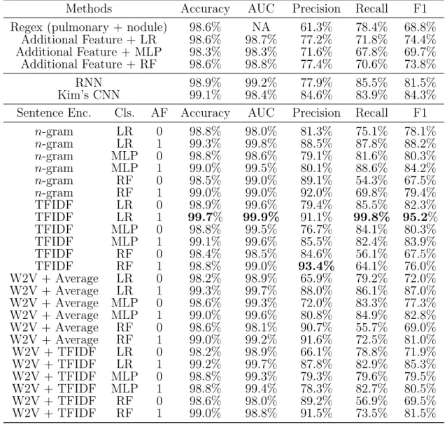
8.3 Experimental Results . . . 114
9.1 Clinical Concept Extraction . . . 120
9.2 Method . . . 121
9.2.1 ELMo Training . . . 122
9.2.2 Bidirectional LSTM CRF model for NER . . . 123
9.3 Experiments and Results . . . 125
9.3.1 Dataset . . . 125
9.3.2 Results . . . 125
10 Summary and Future Directions 128 10.1 Summary . . . 128
10.2 Possible Future Directions . . . 129
References 131
Curriculum Vitae 142
5.1 The encoding of different stimuli and contexts in the context associa-tion task. . . 70 6.1 Numbers of occurrence per anatomical class within the training and
testing corpora. . . 89 6.2 Precision (P), Recall (R), and F1-score on UC 100 dataset. . . 91 6.3 Precision (P), Recall (R), and F1-score on MIMIC 100 dataset. . . 92 7.1 Performance of the negation scope detection task on BioScope corpora
using different approaches. Results are reported as the percentage of the number of predicted scopes that exactly match the golden scope (PCS) . . . 104 7.2 Performance of the negation scope detection task on NegPar corpora
using different approaches. Results are reported as the percentage of number of predicted scopes that exactly match the golden scope (PCS) 104 7.3 Performance of speculation scope detection task on BioScope corpus
using different approaches. Results are reported as the percentage of the number of the predicted scopes that exactly match the golden scope (PCS). . . 105 8.1 Additional features considered for pulmonary nodule finding detection. 111 8.2 Hyperparameters for the Multilayer Perceptron Model. . . 112 8.3 Hyperparameters for the Random Forest Model. . . 112
8.8 Sentence counts in the training and test datasets . . . 115 8.9 Performance of difference algorithms in pulmonary nodule sentence
classification. . . 117 8.10 Some erroneously classified examples by the best pulmonary nodule
classifier. . . 118 8.11 Performance of difference algorithms in incidental finding sentence
clas-sification. . . 118 8.12 Some erroneously classified examples by the best incidental finding
classifier. . . 119 9.1 The corpus statistics for training the ELMo model. . . 123 9.2 Number of reports, sentences, tokens and named entities in training
and test corpora. . . 125 9.3 Performance comparison between the proposed models and the
state-of-the-art models on the 2010 i2b2/VA dataset. . . 126
2·1 Mapping between individual stimuli (A, B, C, D) and the spatial con-text (quadrants 1, 2, 3, 4) onto correct actions X or Y, providing 16 state-action pairs. The underlined (red) state-action pairs are not seen during training but presented during testing. . . 8 2·2 The vector encoding and the sequential encoding for the
stimulus-context pairs. . . 10 2·3 An illustration of the neural networks used inQ-learning. The FC layer
in the diagram represents a Fully-Connected feedforward layer. RNN indicates a Recurrent Neural Network. Q-value est. in the diagram denotes the estimate of the Q-value at the input state for all possible actions. . . 16 2·4 An illustration of the neural networks used in actor-critic learning. The
FC layer in the diagram represents a fully-connected layer. Q-value est. in the diagram denotes the estimate of the Q-value of the state at all possible actions. . . 18 2·5 The hidden state of the feedforward neural networks for the task of
Figure 2·1. The activation function is ReLU, so the hidden state vari-ables are nonnegative. The black dashed line in the figures is the decision boundary determined by the output layer; points above the line correspond to actionY and below the line to action X. . . 22
s2 in time step 2. The black dashed line in the figures in time step 2 is the decision boundary: points above the line correspond to X and points below the line correspond toY. For example, note in Figure (a), stimulus C in the left figure is connected to contexts 2 and 3 in the right figure and map to X. To make the dots easier to differentiate, a small amount of noise was added to the position of the dots in time step 2. . . 23 2·7 The average accuracy (% of correct actions in a test set of input states)
of different models for the context associate task. We tested each algorithm 500 times and averaged the test results. . . 24 3·1 An diagram of the decision-making process of the neural circuit model
for the context association task. The stimulus-context pair ‘A2’ is used and the sequential encoding is applied. For the diagram above, gray entries denote 1 and empty (white) entries denote zero. For illustrative proposes, the noise in the forward propagation is set to zero (= 0). . 28 3·2 The hierarchical decision rule of the neural circuit model demonstrated
for the task of Figure 2·1. The blocks at the three different levels show the state of the hidden neurons at each time instant. The gray block indicates the spiking of the corresponding hidden neuron. . . 43 3·3 Accuracy of the neural circuit model trained by Algorithm 1. . . 44 3·4 Average number of iterations required to converge to an optimal state
with respect to the stepsizeα and the noise strength Unoise. . . 45
4·1 Performances of the neural circuit models with two different update rules. . . 54 4·2 Accuracy of a primal-dual neural circuit. . . 65 4·3 Comparison of generalized task (normalized to 1). The primal-dual
model (top, square symbols) shows perfect generalization accuracy for the context-association task with 4 contexts as shown in Fig. 2·1. . . 65 4·4 Average convergence time as a function of learning rate for primal-dual
training (A) and primal-only training (B). . . 66 4·5 Average convergence time as a function of noise gain for primal-dual
training (A) and primal-only training (B). . . 66 4·6 Average convergence time as a function of the number of hidden
neu-rons for primal-dual training (A) and primal-only training (B). . . 68 5·1 The association rules for the context association task with four contexts. 70 5·2 Accuracy of the model during training . . . 75 5·3 Accuracy and percentage of successful trails under different number of
hidden neurons. . . 76 5·4 Average Accuracy and percentage of successful trails as a function of
the learning rateα and the noise levelµ. . . 76
6·1 A snippet from a radiology report with highlighting of anatomical phrases. . . 78 6·2 A overview of the proposed framework. . . 80
the sequence labeling model as shown in (b). For the given example, the sentence-level label is determined asLung as shown with gray-color box. . . 85 6·4 The sentence encoder model at the document level. A hierarchical
LSTM model is used to produce the sentence-level features. The fea-ture vector produced by the sentence encoder will be used in sequence modeling model as an additional set of features. . . 87 6·5 The anatomy NER results for a set of dummy examples using the best
vanilla model and our model. . . 93 7·1 A diagram of the proposed bi-directional LSTM model for negation
and speculation detection with additional features. . . 99 7·2 A diagram of the proposed BERT-based architecture for negation and
speculation scope detection with inclusion of additional features. . . . 100 7·3 Performance of the BERT models with additional features with respect
to the noise level, averaged over 10 fold cross-validation . . . 106 8·1 Diagram of our proposed framework for incidental finding classification. 109
9·1 The proposed bidirectional LSTM model diagram for medical concept extraction. The char-based CNN word embedding and the bidirectional language model layers (ELMo), shown in the blue color, are pretrained with a corpus from the clinical domain and hold fixed during training the NER model. . . 124
BERT . . . Bidirectional Encoder Representations from Transformers CNN . . . Convolutional Neural Network
CRF . . . Conditional Random Fields
ELMo . . . Embeddings from Language Model GloVe . . . Global Vectors for Word Representation GRU . . . Gated Recurrent Units
LSTM . . . Long Short-Term Memory NER . . . Named Entity Recognition NLP . . . Natural Language Processing NMDA . . . N-Methyl-D-Aspartate
RNN . . . Recurrent Neural Network
R2 . . . the Real plane
TFIDF . . . Term Frequency–Inverse Document Frequency UMLS . . . Unified Medical Language System
Chapter 1
Introduction
It is well known that an object may have a different meaning under different contexts. For examples, when a tick mark is shown as an annotation, people from many English-speaking countries believe it indicates ‘Yes’ while people from Finland, Sweden, and Japan use it as error mark to indicate ‘No’ (Wikipedia contributors, 2018b). One must determine what a tick mark means after knowing what is the context. This phenomenon also appears in linguistics, where a word or phrase has different meaning under different contexts. For example, the word ‘play’ can mean ‘match’ (a football play), or ‘drama’ (a Shakespeare play), or even ‘perform’ as a verb (play the violin) etc. (Wikipedia contributors, 2018a). Therefore, understanding the context is important for making a wise decision for many tasks.
Humans are capable to learn new rules from some examples and summarize and generalize what they have learned. The generalization ability means interpreting previously unseen sensory input to make a correct decision based on a previously learned rule (Fodor and Pylyshyn, 1988). To learn new rules, the neural circuit in cortical, especially the prefrontal cortex are believed to play a very important role (Miller and Cohen, 2001; Wallis et al., 2001). The ability requires some form of symbolic processing for the neural circuit to flexibly apply learned rules to new input. There are various models in the literature characterizing the way neural circuits form a link between an unseen sensory input and the correct response. In this work, a flexible gating mechanism between different cortical working memory buffers by the
basal ganglia (Kriete et al., 2013) and the flexible routing in the prefrontal cortex (Miller and Cohen, 2001) are considered. Three neural circuit models are proposed similar to the one in (Hasselmo and Stern, 2018). These models gate neurons on the synaptic spread of activity between other neurons by interacting populations based on neurons. This gating mechanism can be interpreted as the result of voltage-sensitive conductances, i.e., N-Methyl-D-Aspartate (NMDA) current (Poirazi et al., 2003; Katz et al., 2007). An alternative explanation may be the regulation of the spiking output via axo-axonic inhibitory interneurons (Cutsuridis and Hasselmo, 2012).
Apart from cognitive science, making decisions based on context is also important for clinical natural language processing (NLP). In today’s image-driven care practice, radiology reports are commonly used to capture and store clinical observations and the corresponding interpretations by radiologists and to communicate relevant infor-mation to the primary care physicians and patients. Every observation within the medical images has a corresponding anatomical site of reference. Therefore, a promis-ing approach for the automatic structurpromis-ing of radiology report content is based on the identification and sorting of clinical named entities such as clinical problems, treatments, tests, anatomy sites and its properties such as being negated or hedged. Despite the promising performance of Recurrent Neural Network(RNN)-based mod-els in Named Entity Recognition (NER) (Huang et al., 2015; Ma and Hovy, 2016), capturing the contextual information for inferring anatomy type is a remaining short-coming. For example, consider the following sentence in the: ‘The right lobe of the lung is clear, but the 5mm ground glass nodule in the upper left lobe may require further follow up’. It is straightforward to determine the anatomical label for ‘right lobe of lung’ as it contains the organ name; however, in order to determine the label for ‘upper left lobe’ at the end of the sentence, the anatomy cue existing in ‘right lobe of lung’ at the beginning of the sentence should be taken into account. Based
1.1
Ogranization and Contributions of the Thesis
1.1.1 Reinforcement Learning Methods for Context Association Task
In Chapter 2, a context association task is introduced and different reinforcement learning approaches for the task are considered, including book-keeping reinforcement learning methods, Q-learning and actor-critic learning with linear function and neural network approximation. This dissertation first proves the book-keeping reinforcement learning methods, Q-learning and actor-critic learning methods with a linear function approximation fail to generalize and converge to an optimal solution to the context association task. Then Q-learning and actor-critic learning methods with neural net-work approximation, both fully connected and recurrent, are proposed. Simulation is conducted and the result shows that the Q-learning and actor-critic learning methods with neural networks are able to generalize in the context association task.
1.1.2 Neural Circuit Gating Model for Context Association Task
In Chapter 3, two neural circuit gating models are proposed for the context association task. These models gate neurons on the synaptic spread of activity between other neurons by interacting populations of neurons. The models learn their coefficients using Hebbian learning. For the discrete neural circuit gating model, a convergence guarantee is established when all the examples are provided during training. Finally, simulation is provided to evaluate the performances of both proposed models.
1.1.3 A Recommender-System Inspired Neural Circuit Model for Con-text Association Task
In Chapters 2 and 3, different models for the context association task are provided, but none of them can achieve ideal generalization performance under different num-bers of hidden neurons. In Chapter 4, a novel neural circuit model is proposed for the context association task. The model is inspired by recommender system and two learning methods are provided. Some convergence guarantees are obtained when all the examples are obtained during training for the two learning methods. Finally, some simulation experiments are conducted. The primal-dual learning method, in-spired by the collaborative filtering algorithm in recommender system, achieves a ideal generalization performance.
1.1.4 A Recommender-System Inspired Neural Circuit Model for Con-text Association Task with EZ Rule
In Chapter 4, the neural circuit model achieves an ideal generation performance, but it can only make binary decisions. In Chapter 5, we extend this model to produce multiple responses. A context association task with EZ rule is first proposed, in which three responses are required. Then, we extend the neural circuit model inspired by recommender systems, described in Chapter 4, for multiple responses for the context association task. A learning algorithm is provided based on Hebbian learning. Finally, simulation experiments are conducted to evaluate the performance of the proposed neural circuit model.
1.1.5 Context-based Neural Network Models for Anatomy Name Entity Recognition
In Chapter 6, an anatomy NER problem is first introduced, in which context informa-tion is important for making a good decision. Then, two RNN models are proposed, by
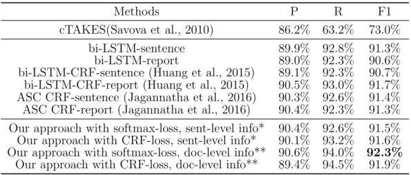
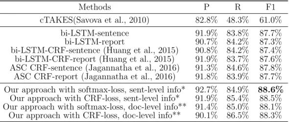
RNN-CRF model is used for producing the token-level features. Finally, we train and evaluate different models in the datasets from two clinical sites and concluded that our proposed models have the best performances among all the models.
1.1.6 Feature-Enrich Neural Token Representations for Negation and Speculation Scope Detection
In Chapter 7, a negation and speculation scope detection problem is considered. A bidirectional Long short-term memory (LSTM) model and a BERT-finetuned model are proposed and different neural token representations, including word embedding and contextual word embedding, are included in the model. In addition, some syn-tactic and semantic features are taken into account to enrich token representation. Finally, two negation and speculation detection datasets are used for evaluation and the proposed models established a state-of-art result.
1.1.7 Incidental Finding Classification for Pulmonary Nodule in Radiol-ogy Report
In Chapter 8, an incidental finding classification problem is introduced for pulmonary nodules in the radiology reports. A two-stage method is proposed to decompose the classification problem into two problems. A sentence classification problem for pul-monary nodule finding is first performed, followed by a classification task for incidental findings. Different sentence classification models are considered, including traditional machine learning and deep learning methods. Also, some additional features includ-ing the anatomy NER model in Chapter 6 and regular expression-based features are taken into account. The models are trained and validated in a real-world dataset and the performances of the models are compared.
1.1.8 Clinical Concept Extraction with Contextual Word Embedding
Automatic extraction of clinical concepts is an essential step for turning the un-structured data within a clinical note into un-structured and actionable information. In Chapter 9, we propose a clinical concept extraction model for automatic annotation of clinical problems, treatments, and tests in clinical notes utilizing domain-specific contextual word embedding. A contextual word embedding model is first trained on a corpus with a mixture of clinical reports and relevant Wikipedia pages in the clinical domain. Next, a bidirectional LSTM-CRF model is trained for clinical con-cept extraction using the contextual word embedding model. We tested our proposed model on the I2B2 2010 challenge dataset. Our proposed model achieved the best performance among reported baseline models and outperformed the previous state-of-the-art models by 3.4% in terms of F1-score.
Chapter 2
Reinforcement Learning Methods for a
Context Association Task
In this chapter, the context association task, which is first introduced in (Raudies et al., 2014) and later analyzed in (Hasselmo and Stern, 2018), is first introduced. Two different types of reinforcement learning methods are proposed for this task. Simulation experiments are conducted to access the performance of the reinforcement learning methods on the context association task.
Considerable recent research has focused on the strength of deep reinforcement learning (Mnih et al., 2015; Hausknecht and Stone, 2016; Mnih et al., 2016). This recent work returns to the use of neural networks as function approximators in the context of reinforcement learning, first considered by Tesauro (Tesauro, 1994), but introduces deep architectures instead of the earlier multilayer perceptron with one hidden layer used in (Tesauro, 1994). Arguably, this represents a break from a body of work considering function approximators as linear combinations of hard-to-engineer nonlinear feature functions (Bertsekas, 1996).
It is therefore worthwhile to consider the mechanisms by which deep reinforce-ment learning could be used to perform complex cognitive task modules for associa-tions between stimuli and responses. The recent work mentioned above, has shown that deep learning techniques coupled with reinforcement learning algorithms can learn decision making over a high-dimensional state space such as images in a video game (Mnih et al., 2015; Hausknecht and Stone, 2016; Mnih et al., 2016). In (Mnih
et al., 2015), the deepQ-network is used to train a reinforcement learning agent play-ing Atari games usplay-ing game images. (Mnih et al., 2016) further develops this idea into actor-critic learning and also proposes a parallel computing scheme for reinforcement learning. The neural networks in these models enable the learning agent to make decisions hierarchically. The models in these papers all use the traditional neural network elements with continuous values representing the mean firing rate across a population of neurons that increases when the input crosses a threshold (Rumelhart et al., 1988).
2.1
Context Association Task
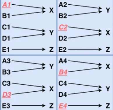
The basic learning task we analyzed was considered in (Raudies et al., 2014). The task aims to evaluate the ability of a learning agent to associate specific stimuli with appropriate responses in particular spatial contexts. Figure 2·1 shows the mapping between input and responses. The input consists of stimuli, denoted by letters A, B, C, and D, and a spatial context corresponding to four quadrants and denoted by numbers 1, 2, 3, and 4. This dissertation will use the term state to refer to the stimulus-context pairs. The two legal responses (or actions) are X and Y.
Figure 2·1: Mapping between individual stimuli (A, B, C, D) and the spatial context (quadrants 1, 2, 3, 4) onto correct actions X or Y, providing 16 state-action pairs. The underlined (red) state-action pairs are not seen during training but presented during testing.
with another context. To test the generalization ability of the various models, some context-stimulus pairs are hidden during training. For the basic task, the hidden states are underlined and in red in Figure 2·1.
The task is designed to test the following abilities for a learning agent: 1) The agent should make a decision, i.e., associating the stimulus with the correct response, based on the context. 2) The agent should generalize beyond what it learned.
Two different presentations (codings) for the state are used in this dissertation, shown in Figure 2·2. The first encoding method is the vector representation intro-duced in (Raudies et al., 2014). It uses a (κ+l)-dimensional binary vector to code the state, where l is the number of contexts and κ the number of stimuli. This dis-sertation will usen =κ+l to denote the dimension of the entire vector encoding the state. Here n = 8 since there are four contexts and four stimuli considered in the task. The firstκ= 4 bits correspond to the stimuli and the lastl= 4 bits correspond to the contexts 1, . . . , l. Each 4-bit codeword uses one-hot encoding to represent the stimulus or context, with one bit being set to one to encode for the corresponding context. Figure 2·2(b) provides an example of this type of encoding for the task of Figure 2·1.
The second representation consists of a sequence of two n-dimensional binary vectors. The first one in the sequence represents the stimulus; for our tasks, bits 1 through κ (= 4) being 1 correspond to stimuli A through D, respectively, while the last l bits are set to zero. The second vector in the sequence has its firstκ bits set to zero and the last l bits, κthrough κ+l, being set to 1 in order to represent contexts 1 to 4, respectively. Figure 2·2(c) shows an example of representing state B3 in the task of Figure 2·1 using a two vector sequence s1,s2. For the proposed neural circuit
models, this type of representation is used.
(a) The encoding of different stimuli and contexts in the task of Figure 2·1. Stimuli and contexts Encoding
Stimulus A (1, 0, 0, 0, 0, 0, 0 ,0) B (0, 1, 0, 0, 0, 0, 0 ,0) C (0, 0, 1, 0, 0, 0, 0 ,0) D (0, 0, 0, 1, 0, 0, 0 ,0) Context 1 (0, 0, 0, 0, 1, 0, 0 ,0) 2 (0, 0, 0, 0, 0, 1, 0 ,0) 3 (0, 0, 0, 0, 0, 0, 1 ,0) 4 (0, 0, 0, 0, 0, 0, 0 ,1)
(b) An example of vector encoding for stimulus-context pairs. Stimulus-context pair: B3, Stimulus B →(0,1,0,0,0,0,0,0), Context 3 →(0,0,0,0,0,0,1,0), Encoded vector: s= (0,1,0,0,0,0,1,0).
(c) An example of sequential encoding for stimulus-context pairs.
Stimulus-context pair: B3,
Stimulus B →(0,1,0,0,0,0,0,0), Context 3 →(0,0,0,0,0,0,1,0), Encoded time series:
s1 = (0,1,0,0,0,0,0,0),
s2 = (0,0,0,0,0,0,1,0).
Figure 2·2: The vector encoding and the sequential encoding for the stimulus-context pairs.
2.2
Q
-Learning Algorithms
In this section, we will introduce theQ-learning algorithm and its variants for solving the discounted MDP problem. Q-learning (Watkins and Dayan, 1992) is a method for solving (2.3) and can be used even in the absence of an explicit model for a MDP. Essentially, Q-learning solves (2.3) using a value iteration method but with the expectation with respect to the next state being approximated by sampling. The original Q-learning algorithm iterates over the Q-factors at all states and actions, which is computationally intractable for large MDPs. Approximate versions of the method have been introduced (see (Bertsekas, 2012; Bertsekas, 1996)), where the
who is continuously being presented with states (the stimuli-context pairs) and pro-duces an action (response) that can be eitherX orY. Given a state and the selected action, the agent transitions to a next state which simply corresponds to the next state at which the agent is asked to produce a response. We will use a discrete-time
Markov Decision Process (MDP)(Bertsekas, 2012; Bertsekas, 1996) to represent this learning process.
The MDP has a finite state space S, consisting of the states and an action space
U, consisting of the actions X and Y. Let sk ∈ S and uk ∈ U be the state and the
action taken at time k respectively, and let s0 be an initial state of the MDP. Let
p(sk+1|sk, u) denote the probability that the next state issk+1, given the current state issk and action uis taken. We assume, without loss of generality in our setting, that
these transition probabilities are uniform in all non-hidden states for all states and actions.
When the agent selects a correct action, it receives a reward; otherwise, it gets penalized. Let g(sk, uk) be the one-step reward at time k when action uk is selected
at statesk. We define the one-step reward to be 1 ifuk is the correct response at state sk and −4 otherwise. We seek apolicy, which is a mapping from states to actions, to
maximize the long-term discounted reward ¯ R= ∞ X k=0 γkg(sk, uk), (2.1)
where, from now on, we will use a discount rate of γ = 0.9.
starting from s. The value function satisfies the following Bellman’s equation V(s) = max u g(s, u) +γX q∈S p(q|s, u)V(q) . (2.2)
Given a solutionV∗(·) to (2.2), one can easily find the optimal action u∗ at each state
s as the maximizing u in (2.2) and thatu∗ will necessarily be the correct action. Define now the so-calledQ-factor which is a function Q(s, u) of state-action pairs and is equal to the maximum long-term reward obtained starting fromsand selecting as first actionu. The Q-factor also satisfies a recursive equation, namely
Q(s, u) = g(s, u) +γX q∈S
p(q|s, u) min
v Q(q, v). (2.3)
From a solution, say Q∗(·,·), of (2.3) one can also obtain the optimal action at each state s asu∗(s) = arg minu∈UQ(s, u).
2.2.2 Original Q-Learning Algorithm
The original Q-learning algorithm updates the Q-factors as follows:
Qk+1(sk, uk) =Qk(sk, uk)−λkTDk
TDk =Qk(sk, uk)−γmin
u Qk(sk, u)−g(sk, uk), (2.4)
whereλk is a Square Summable but Not Summable (SSNS) step-size sequence, which
means λk > 0, P ∞ k=0λk = ∞, and P∞ k=0λ 2
k < ∞. The actions uk can be chosen
according to anε-random policy, i.e., with probabilityε, choose a random action and with probability 1−ε, choose an action minimizingQk(sk,·). The algorithm maintains
allQ-factor estimates for all state-action pairs during the training processes. Hence, it requires a large amount of memory and a long training time if the number of the state-action pairs is excessive (Bertsekas, 2012).
task we are considering. A negative result is shown in the next theorem.
Theorem 2.1. The Q-factors obtained by the Algorithm in (2.4) do not converge to the optimal Q-factor Q(s, a) for the MDP of the learning task in Subsection 2.1 if the initial Q0(s, a)=6 Q(s, a) for any s included in the hidden states.
Proof: According to the updating rule of the Q-learning, the Q-factor for state-action pair (s, a) can be updated ifsk =s and ak =a for some k. However, hidden
states are not shown during the training. Hence, Q-factors for state-action pairs (s, a), where s is a hidden state are never updated from their initial states. Thus, if their initial values are not optimal, the Q-factors obtained by the Algorithm in (2.4) do not converge to their optimal values for all state-action pairs. Therefore, the original Q-learning algorithm can not learn the optimal policy of the learning task. This is because the original Q-learning maintains a look-up table for Q-factors of all state-action pairs and can not generalize by using previous seen examples.
2.2.3 Q-Learning with Linear Function Approximation
To reduce the large memory used by the look-up table representation in the original
Q-learning algorithm, linear function approximation emerged as an alternative. A linear function approximation is used, since it is simple and leads to convergence results (Bertsekas, 2012; Bertsekas, 1996). The algorithm approximates theQ-factors as
˜
Q(s, a) =φ(s, a)0θ (2.5)
where φ(s, a) is a feature vector of the state-action pair of the MDP and θ is a parameter vector obtained iteratively during theQ-learning. The performance of this method depends heavily on the selection of the features. As we show later, even
when using a set of features that contain sufficient information regarding the future costs/rewards associated with a state-action pair, the linear architecture fails to find an optimal policy.
We use the vector encoding of the state, shown in Subsection 2.1, to construct features. Since this is only a feature for the state, it needs augmentation to account for actions as well. To that end, we use the following Q-factor estimate:
˜ Q(s,X) ˜ Q(s,Y) =Θx(s), (2.6)
where Θ ∈ R2×8 is a parameter matrix and x(s) ∈
R8 is the vector encoding of the
state s. Notice that this approximation is a special case of (2.5).
Theorem 2.2. The Q-factors obtained by the Q-learning algorithm under the linear function approximation in (2.6) are not optimal for the MDP of the learning task in Subsection 2.1. Moreover, the policy obtained by this algorithm is not optimal.
Proof: We will show that the policy obtained from the Q-factors derived by this algorithm does not agree with the optimal one. Suppose we find a Q-factor function in the form (2.6) that selects the optimal actions for all states. From Fig. 2·1, it follows: ˜ Q(A1,X)>Q˜(A1,Y), (2.7) ˜ Q(A2,X)<Q˜(A2,Y), (2.8) ˜ Q(C1,X)<Q˜(C1,Y), (2.9) ˜ Q(C2,X)>Q˜(C2.Y). (2.10)
From Fig. 2·2, we obtain
x(A2)−x(A1) +x(C1) =x(C2). (2.11)
formation regarding a state, Q-learning may not always produce the correct answer. This is because the linear function approximation does not have the ability to make decisions hierarchically. This result can be easily generalized to affine functions as well. Hence, Q-learning relies heavily on the feature selection, with the latter being more of an art and very much problem specific.
2.2.4 Q-Learning with Neural Network-based Function Approximation
To avoid feature engineering, neural networks offer an alternative for learning ap-proximations of the value function, or the Q-factor, or even the policy directly. Deep learning is making major advances in solving problems that have resisted the best attempts of the artificial intelligence community for many years (LeCun et al., 2015). The advance of deep learning makes it possible to use deep neural networks to approx-imately solve the MDP efficiently. One such method is the deep Q-network (DQN), proposed in (Mnih et al., 2015). The main idea is to use a deep neural network to approximate the Q-factor function and obtain the neural network weights using Q -learning. Following this line of work, (Mnih et al., 2016) proposed an asynchronous method forQ-learning and actor-critic learning, on which the Q-learning method we use for our learning task is based. Though the neural network used for our task is not deep and only contains one thread, it provides some insight on the ability of neural networks to generalize as is needed in the task we consider.
The algorithm we use for Q-learning with a neural network is showed in Algo-rithm 1 in (Mnih et al., 2016). We only use the algoAlgo-rithm in (Mnih et al., 2016) with a single agent. It uses a neural network to approximate the Q-factor of the MDP. The neural network takes as input the state and outputs the estimated Q-factor of the state and each possible action. In particular, in this dissertation we compare
two kinds of neural networks (Goodfellow et al., 2016) to approximate the Q-factor. The first one is a feedforward neural network, which consists only ofFully-Connected (FC)layers and inputs in the vector encoding form of Fig. 2·2(b). The second neural network is a so-called Recurrent Neural Network (RNN), which accepts inputs in the sequential encoding of Fig. 2·2(c) and produces an estimate of the Q-factor.
(a)An illustration of the neural net-work for Q-learning using vector en-coded input.
(b)An illustration of the neural net-work for Q-learning using sequen-tially encoded input.
Figure 2·3: An illustration of the neural networks used in Q-learning. The FC layer in the diagram represents a Fully-Connected feedforward layer. RNN indicates a Recurrent Neural Network. Q-value est. in the diagram denotes the estimate of the Q-value at the input state for all possible actions.
In the feedforward network, the input is the vector encoded states; an vector of 8 dimensions. The output is the Q-factor at each possible action in that state, that is, the 2-dimensional vector (Q(s, X), Q(s, Y)). The activation functions of the neurons are all Rectified Linear Units (ReLU), except for the output layer (Nair and Hinton, 2010). In particular, ReLU(x) = max(x,0), for some vector x, where the maximum is taken element-wise. There is no activation function in the output layer, since the
q=W2h+b2,
whereW1 ∈Rm×8 is the weight matrix of the first fully-connected layer, W2 ∈R2×m is the weight matrix of the second fully-connected layer, and b1 ∈ Rm, b2 ∈R2, are
additional parameters of the first and second layers we need to learn. Here, m is the number of hidden neurons in the first fully-connected layer and q is the estimate of (Q(s, X), Q(s, Y)). A diagram of this structure can be found in Figure 2·3a
Next, we turn to the RNN architecture. The input, in this case, uses the sequen-tial encoding and is a sequence of two vectors s1,s2 ∈ R8 as shown in Fig. 2·2(c). The output, similar as above, is the Q-factor at each possible action in that state, i.e., (Q(s, X), Q(s, Y)). For simplicity, we use a neural network with a simple RNN layer and a fully-connected layer to approximate the Q-factor. Letting s1,s2 be the sequential encoding of the input states,h1,h2 the outputs of the first and the second RNN layers, andq the output of the FC layer, we have
h1 = ReLU(W11s1 +W12h0), (2.13)
h2 = ReLU(W11s2 +W12h1),
y=W2h2+b2,
where the initial state of the RNN ish0 =0,W
11∈Rm×8,W12∈Rm×m,W2 ∈R2×m and b2 ∈ R2 are parameters we wish to learn, m is the number of the hidden states
in the simple RNN layers, and yis the estimate of (Q(s, X), Q(s, Y)). A diagram of the proposed model can be found in Figure 2·3b
(a)An illustration of the neural net-work for actor-critic learning using the vector encoding of the state.
(b)An illustration of the neural net-work for actor critic learning using the sequential encoding of the state. Figure 2·4: An illustration of the neural networks used in actor-critic learning. The FC layer in the diagram represents a fully-connected layer. Q-value est. in the diagram denotes the estimate of the Q-value of the state at all possible actions.
2.3
Actor-Critic Learning Using Neural Networks
The actor-critic algorithm is also a type of reinforcement learning algorithm. It posits a parametric Randomized Stationary Policy (RSP) and rather than seeking an optimal policy, it seeks an optimal parameter vector for the RSP. Traditionally, actor-critic learning uses a logistic function for the policy which leads to a linear function approximation for the Q-value function (Konda and Tsitsiklis, 2000). In particular, the policy is specified through a probability for selecting actionu at state s given by
µθ(u|s) = exp{θ0φ(s, u)} P vexp{θ 0 φ(s, v)}, (2.14)
where θ is a parameter vector and φ(s, u) is a vector of features of the state and the action. The operation on the right hand side of (2.14) which assigns the highest probability to the action that maximizes the exponent θ0φ(s, u) is often referred to asSoftmax. Specifically, for some vectorx= (x1, . . . , xk)∈Rk, Softmax(x)∈Rk and
Pk
j=1exp(xj)
i= 1, . . . , k. It can be shown (Konda and Tsitsiklis, 2000), that given an RSP as in (2.14), a good linear approximation of the Q-value function is Qθ(s, u) = r0ψθ(s, u) where ψθ(s, u) =∇lnµθ(u|s).
The actor critic method alternates between an actor step which is a gradient update of the parameter vector θ using the gradient of the long-term reward, and a critic step which, given the current θ, uses Temporal-Difference (TD) learning (Pennesi and Paschalidis, 2010; Sutton, 1988) to learn the appropriate parameter r
in the Q-value function approximation in addition to the long-term reward and its gradient with respect to θ. As we commented earlier when discussing Q-learning, these methods have been shown to converge (Konda and Tsitsiklis, 2000) but depend on proper selection of feature functions in order to be effective.
If instead one uses a neural network to approximate the value function and the policy, the actor-critic updating steps should be modified. For example, (Hausknecht and Stone, 2016) proposed a deep actor-critic learning similar to the DQN. (Mnih et al., 2016) used a simpler way, updating a loss function that combines the policy advantage and a temporal-difference term for the value function.
In this dissertation, we use the actor-critic learning algorithm of (Mnih et al., 2016) to handle the learning tasks we introduced in Sec. 2.1. The neural network takes as input the statesof the MDP, and outputs both a policy and a value function estimate. As we did with Q-learning, we will use both a feed-forward neural network and an RNN version of the algorithm. Again, we only use the actor-critic learning algorithm in (Mnih et al., 2016) with a single agent.
learning is shown in Figure 2·4. For the policy, we use a fully-connected layer with a Softmax activation function. For the value function, we use an additional fully-connected layer without an activation function. Lettingsthe vector encoded state, h
the output of the the first FC layer,v the output of the FC layer producing the value function estimate, and µ the output of the FC layer producing the policy estimate, we have
h= ReLU(W1s+b1), (2.15)
µ= Softmax(Wµh+bµ),
v =Wvh+bv,
where W1 ∈ Rm×n, b1 ∈ Rm, Wµ ∈ R2×m, bµ ∈ R2, Wv ∈ R1×m and bv ∈ R are
the parameters in the neural networks we need to learn, and m is the number of the hidden neurons in the first FC layer.
In the RNN case, and similar to theQ-learning case, we lets1,s2 be the sequential encoding of the input state s, h1,h2 the outputs of the first and the second RNN layers, v the output of the FC layer producing the value function estimate, andµthe output of the FC layer producing the policy estimate, which leads to
h1 = ReLU(W11s1 +W12h0), (2.16)
h2 = ReLU(W11s2 +W12h1),
µ= Softmax(Wµh2 +bµ),
v =Wvh2+bv, (2.17)
where the initial state of the RNN is h0 = 0, W
11 ∈ Rm×n, W12 ∈ Rm×m, Wµ ∈
R2×m,Wv ∈R1×m, bµ∈R2 and bv ∈Rare parameters to learn andm is the number
of neurons (Dayan and Abbott, 2001). This has many advantages, such as graceful degradation when individual neurons are lost. However, the distributed representa-tion makes it difficult to interpret the activity patterns in trained models. In order to overcome this difficulty, this dissertation uses two approaches to investigate the performance of different methods. The first one is a minimalist approach, which tries to use the simplest model to train the Q-learning agents. Using the least number of units and parameters, it becomes easier to understand how these methods solve the learning task of Subsection 2.1. The other approach is to use a larger numbers of neurons to learn the task since the real neural system encodes the information in a distributed manner. We will compare the performance of each model across different numbers of units and seek to discover potential relationships among these methods.
First, we test the Q-learning and actor-critic learning algorithm with function ap-proximation using a feedforward neural network (2.12). For minimalism, we use only 2 hidden neurons in the hidden layer. For training the network we use Algorithm 1 in (Mnih et al., 2016). We visualize the decision rule for a set of learned parameters which are successful in selecting a correct action even at the 4 states which are not seen during training. The values associated with the 2 hidden neurons h = (h1, h2) are shown in Fig. 2·5.
Next, we test the Q-learning algorithm using sequentially-encoded input (2.13). Again, the neural network we use has 2 hidden neurons in each simple RNN layer. Using the same setting, the learned model successfully makes each generalization and finds the correct answer. We visualize its decision rule in Fig. 2·6.
Finally, we tested the Q-learning algorithm and actor-critic learning using differ-ent numbers of hidden neurons. It is known that biological neural systems encode
(a) Q-learning using the vector-encoded input.
(b) Actor-critic learning using vector-encoded input.
Figure 2·5: The hidden state of the feedforward neural networks for the task of Figure 2·1. The activation function is ReLU, so the hidden state variables are nonnegative. The black dashed line in the figures is the decision boundary determined by the output layer; points above the line correspond to action Y and below the line to actionX.
information in a distributed manner. One pattern of information may be encoded by many neurons. This encoding may not be very efficient (Dayan and Abbott, 2001), but increased numbers of units may help in the learning procedure. We changed the number of the hidden neurons to assess its effect on the performance of the neural network. We used the following settings for the various parameters of the Q-learning and actor-critic algorithm. We used the Adam optimizer (Kingma and Ba, 2014) with a learning rate of 0.05, β1 = 0.9,β2 = 0.999, = 10−8. The discount factor was
γ = 0.9 for Q-learning. We let the algorithm update every 100 actions. The maxi-mum learning step was set to 50,000 actions. Shown in Fig. 2·7 is the performance of the two methods we described so far in this section as we vary the number of hid-den neurons. In the figure, “Q-learning (FC)” corresponds to the method in (2.12) with the vector-encoded input. “Q-learning (RNN)” corresponds to the method in (2.13) with the sequentially-encoded input. Similarly, “actor-critic learning (FC)” corresponds to the actor-critic learning method with the vector-encoded input and
(a) Q-learning using the simple RNN.
(b) Actor-critic learning using the simple RNN.
Figure 2·6: The hidden state of the simple RNN for the task of Fig-ure 2·1. The activation function is ReLU, so the hidden state variables are nonnegative. The linkage between the two time steps in the cor-responding figures indicates that a state s1 in time step 1 is precursor of a state s2 in time step 2. The black dashed line in the figures in time step 2 is the decision boundary: points above the line correspond to X and points below the line correspond to Y. For example, note in Figure (a), stimulus C in the left figure is connected to contexts 2 and 3 in the right figure and map to X. To make the dots easier to differentiate, a small amount of noise was added to the position of the dots in time step 2.
“actor-critic learning (RNN)” corresponds to the actor-critic learning with sequence-encoded input. For all four experiments, by increasing the number of hidden neurons we improve the performance of the learning process.
Figure 2·7: The average accuracy (% of correct actions in a test set of input states) of different models for the context associate task. We tested each algorithm 500 times and averaged the test results.
Chapter 3
Neural Circuit Gating Model for the
Context Association Task
In Chapter 2, a set of reinforcement learning methods are proposed for the context association task. However, the biological plausibility of reinforcement learning mod-els with neural networks is questionable, since the biological brain do not appear to perform a backwards propagation. In this chapter, we consider two types of neu-ral circuit model trained using Hebbian learning, and show convergence of Hebbian learning in one neural circuit model. Simulations are also provided for supporting the theoretical results.
3.1
Neural Circuit Models for Context Association Task
In this section, three neural circuit models are proposed for the context association task.
3.1.1 A Class of Continuous Neural Circuit Gating Models
First, a neural circuit gating model will be presented using neurons with simple step-function threshold dynamics that could be considered similar to the generation of single spikes in individual neurons. These single spikes then gate the spread of activity between other neurons by altering the weight matrix. Our neural circuit model is defined next, which is based on the model presented in (Hasselmo and Stern, 2018). An illustrative example of this model and how it operates for the context association
task can be found in Figure 3·1.
With regard to biological justification, this gating mechanism is based on the non-linear effects between synaptic inputs on adjacent parts of the dendritic tree that are due to voltage-sensitive conductances such as the N-Methyl-D-Aspartate (NMDA) current (Poirazi et al., 2003; Katz et al., 2007). These interactions could allow synap-tic input from a spiking neuron to determine whether adjacent neurons have a signif-icant influence on the membrane potential. Here, this is represented by the spiking of hidden neurons directly gating the weight matrix. Alternatively, these effects could be due to axo-axonic inhibition gating the output of individual neurons.
Learning parameters for this model are based on the Hebbian rule for plasticity of synaptic connections. Previously, (Hasselmo, 2005) presented a neurobiological circuit model with gating of the spread of neural activity combined with local Hebbian learning rules and suggested it could have functions similar to TD learning. In this dissertation, we present another neural circuit model based mostly on Hebbian rules, which has a performance comparable to the more abstract neural network models. Our neural circuit model is defined next. An illustrative example of this model and how it operates for the context association task can be found in Figure 3·1.
We will use the sequential encoding of the state as input, where a state s is presented as a sequence of twon-dimensional vectorss1 ands2. We havenneurons to receive these signals. In addition to the input neurons, we usem= 5 hidden neurons to process the information. Three of these neurons store an internal state and two are used to output actionsX andY (see Fig. 3·1(b)). We denote byat
i the activation
of neuron iat time t;at
i = 1 if the neuron gets activated and is zero otherwise. Here, i = 1, . . . , n corresponds to the input neurons and i =n+ 1, . . . , n+m corresponds to the hidden neurons. We let at = (at
1, . . . , atn+m). For simplicity, we assume there
reflects the nonlinear interaction of synapses on the dendritic tree, in which activation of one synapse can allow an adjacent synapse with voltage-sensitive conductances to have an effect. The weight matrix of the neural network is denoted asWj ∈Rm×(n+m),
when hidden neuron j is spiking. Let
ft=Wjat, (3.1)
where j ={i| at
i = 1} is the index of the activated hidden neuron at time t. Notice
that the activated hidden neuron determines the weight matrix to be used. We assume these iterations start with the first hidden neuron being activated at t = 1, namely
a1 = (s
1,1,0,0,0,0).
To determine the state of the hidden neurons (atn+1+1, ant+1+2, atn+1+3) at timet+ 1, we use the following probabilistic model. With a small probability ε, we randomly pick one of these hidden neurons to emit a spike at time t + 1. Otherwise, we let the neuron k = n+ 1, n+ 2, n+ 3 with the highest fkt to emit a spike. This procedure can be interpreted as a balance of exploration and exploitation in the reinforcement learning context (Bertsekas, 2012; Bertsekas, 1996).
The last two hidden neurons (atn+4, atn+5) represent selection of either actionX or action Y. Specifically, (at
n+4, atn+5) = (1,0) selects action X and (atn+4, atn+5) = (0,1) action Y. Otherwise, no action is implemented.
An example of the decision-making process using the neural circuit is shown in Figure 3·1. This example uses the stimulus-context pair A2 as input, provided in the form of the sequential encoding s1,s2. For illustrative proposes, the noise is always set to zero. The first hidden neuron is activated by default at t = 1. The encoded input for stimulus A spreads across this weight matrix W1 gated by the
(a) The decision-making process using the neural cir-cuit gating model.
(b) An interpretation of the hidden states. Figure 3·1: An diagram of the decision-making process of the neural circuit model for the context association task. The stimulus-context pair ‘A2’ is used and the sequential encoding is applied. For the diagram above, gray entries denote 1 and empty (white) entries denote zero. For illustrative proposes, the noise in the forward propagation is set to zero (= 0).
matrix W2 is applied to a2 = (0,0,0,0,0,1,0,0,0,1,0,0,0). With the coded input of context 2, the activity spreads across the weight matrix to generate an output in which the fifth hidden neuron is activated, corresponding to action Y.
To learn the weight matrices Wi we follow the properties of the Hebbian learning
rule. The synapses are updated by reward-dependent Hebbian Long-Term Poten-tiation (LTP), in which active synapses are tagged based on the presence of joint pre-synaptic and post-synaptic activity, and then, the synapse is strengthened if the output action matches the correct action. Long-Term Depression (LTD) provides an activity-dependent reduction in the efficacy of neuronal synapses to serve as a regularization of the learning process.
The LTP rule is mostly based on the basic Hebb rule in (Dayan and Abbott, 2001), in which simultaneous pre- and post-synaptic activity increases synaptic strength. In particular, suppose the it hidden neuron is activated at time t. Let ath denote the
vector consisting of the lastmcomponents ofat, corresponding to the hidden neurons.
Then the LTP term is
∆Wit,LTP =a t0 ho t , whereot ∈
Rm indicates the spiking of hidden neuron at time t. In particular, we let
oti = 1 if hidden neuron iis activated at timet, andoti = 0 otherwise. The LTD term is ∆Wit,LTD=−(a t h) 0 e
where e∈Rm is the vector of all 1’s.
Finally, the weight matrices Wi are updated as follows. For a given input signal,
update the weight matrices Wi1 and Wi2 as
Wit,t+1 =Wit,t+αLT P∆Wit,LTP+αLT D∆Wit,LTD (3.2)
where αLT P and αLT D are appropriate stepsizes. Since this updating rule is not
necessarily stable, we project the elements of Wi to [0,1] after every update.
3.1.2 A Discrete Neural Circuit Gating Model
The first type of the neural circuit model we presented is biologically plausible but has a number of drawbacks. First, even though all the neurons perform a certain task, the number of neurons is more than what is needed. Second, it is hard to characterize the convergence properties of the neural circuit model, i.e., if all the data are provided during the training, is it able to converge to some model that performs correctly for all stimulus-context pairs?
In this section, a discrete neural circuit model is provided to overcome the draw-backs described above. Compared with the model in the last section, this one uses a more compact neural circuit design and has a finite number of possible weight matri-ces in the neural circuit. These will make it possible to characterize the convergence property of the neural circuit.
The input to the neural circuit model is the stimulus-context pair swe described earlier, represented as a sequence (s1,s2) of two 8-dimensional vectors. The model has n = 8 neurons that receive such input sequences in two time instances. In addition, there arem≥2 hidden neurons andmweight matrices connecting the input neurons and the hidden neurons; these weight matrices are denoted by Wi ∈ Rm×n, i= 1, . . . , m.
For each inputs, the model makes a decision in two time steps denoted byt= 1,2.
{0,1}m the indicator vector associated with the activation of hidden neurons at time t; specifically, at,i = 1 if neuron i spikes at time t and is zero otherwise. At each
time instance, there is only one hidden neuron spiking. We denote byit the activated
neuron at time t, i.e., it = arg maxiat,i.
The decision-making rule of the neural circuit model is described as follows. We assume neuron 1 is spiking initially, i.e., a0,1 = 1. At each time instance t, the pre-activation functionft= (ft,1, . . . , ft,m) of the hidden neurons is defined as
ft=Wit−1st+ωt, (3.3) at,i =
1, if i= arg maxift,i,
0, otherwise,
(3.4)
where ωt∈Rm is an environment noise with each element independent of the others
and uniformly distributed in [0,1). (Ties in (3.4) are broken arbitrarily.) We assume
ωt are independent for different times t. Notice that the activated hidden neuron
at the previous time instance determines the weight matrix to be used. The spiking neuron at t is the neuron that has the maximum pre-activation value.
At the last time instance for each input (t = 2), the last two hidden neurons determine the selection of either responseXor responseY. Specifically, ifa2,m−1 = 1, then responseX is selected. If a2,m = 1, then responseY is selected. If the activated
neuron is not one of the last two, then no response is provided.
We provide an example to illustrate the operation of the neural circuit model. Suppose there are two hidden neurons (m = 2) and the two corresponding weight
matrices are: W1 = 1 1 0 0 1 0 0 1 0 0 1 1 0 1 1 0 , W2 = 0 0 0 0 0 1 1 0 0 0 0 0 1 0 0 1 . (3.5)
Suppose the input is the stimulus-context pair C1 and the noise ωt = (0,0). The
input at the first time instance is s1 = (0,0,1,0,0,0,0,0). Then, the pre-activation function becomes f1 = W1s1 = (0,1). Therefore, a1 = (0,1) and the second hidden neuron spikes at time t = 1. The input for t = 2 is s2 = (0,0,0,0,1,0,0,0) and
f2 = W2s2 = (0,1). Hence, a2 = (0,1) and response Y is selected since it is the second hidden neuron spiking at the final time instance t = 2. It can be verified that the weight matrices in (3.5) will always yield the correct response for every stimulus-context pair input according to the context association task.
To train the weight matrices, We devise a learning algorithm for the neural cir-cuit based on the Hebbian rule for plasticity of synaptic connections. The weight matrices Wi are updated according to a combination of LTP and LTD, modulated
by appropriate gating and depending on whether the output response matches the correct one.
The LTP rule is mostly based on the basic Hebbian rule in (Dayan and Ab-bott, 2001), in which simultaneous pre- and post-synaptic activity increases synaptic strength. Recall thatitis the index of the spiking hidden neuron at timet,t= 0,1,2.
According to our assumption, i0 = 1. The LTP term is:
∆Wit−1,LTP=ots
0
t. (3.6)
t−1 t
Finally, the following update rule is considered for this neural circuit model. Given an input signal, if the response of the neural circuit model coincides with the correct response, the LTP rule is applied for updating the weight matrices. Otherwise, when either the response is incorrect or there is no response produced, the LTD rule is applied. Finally, the elements of the weight matrices Wi are projected to [0,1] after
every update. Algorithm 1 specifies the steps of the learning algorithm, where α ∈
(0,1) is a stepsize.
Algorithm 1 Hebbian Learning Algorithm for the neural circuit model.
Initialization: Initialize Wi =0, i= 1, . . . , m. repeat
Sample a state s. Set i0 = 1.
for t = 1,2do
Find the spiking neuron at time t using (3.3) and (3.4). Set ∆Wit−1,LT P, ∆Wit−1,LT D according to (3.6) and (3.7).
end for
Select response X or Y according the spiking neuron at t= 2.
if the response is correct then
Perform an LTP update for the weight matrices
Wit−1 ←Wit−1 +α∆Wit−1,LT P, t= 1,2.
else
Perform an LTD update for the weight matrices
Wit−1 ←Wit−1 +α∆Wit−1,LT D, t= 1,2.
end if
Project all elements ofWi to [0,1],∀i= 1, . . . , m. untilsome convergence criterion on Wi is satisfied.
Theorem 3.1. The neural circuit model converges to an optimal state under Algo-rithm 1 if each input (stimulus-context pair) is sampled in AlgoAlgo-rithm 1 uniformly.
The proof to Theorem 3.1 is shown in the next subsection.
3.1.3 Convergence of the Neural Circuit Gating Model
In this section, we establish the convergence of Algorithm 1 for the context association task we have introduced. To that end, we will consider a discrete-time Markov chain whose “state” is characterized by the weight matrices. We will use xt to denote the
state of a (generic) Markov chain at timet. We make the following assumption about the inputs provided to the algorithm.
Assumption 3.2. Each input (stimulus-context pair) is sampled in Algorithm 1 uni-formly.
In fact, it suffices to sample any input with a constant positive probability at each time; we assume a uniform sampling distribution for simplicity.
Definition 3.3 ((Br´emaud, 2013)). A state i in a Markov chain is called closed, if
P(xt+1 =i|xt = i) = 1. We say a state i is accessible from a state j, if there exists
some T >0, such that P(xt+T =i|xt=j)>0.
The following lemma follows from standard Markov chain theory. We omit the proof.
Lemma 3.4. Consider a Markov chain with a finite state space X. Let Xc be the
set that contains all its closed states. Suppose that for all states i ∈ X, there exists somej(i)∈ Xc such that j(i) is accessible from i. Then, for every initial distribution
of the Markov chain, a stationary distribution exists and is such that all elements corresponding to non-closed states are zero.
Proof: According to Definition 3.3 and the above assumption, for all state i ∈ X, there exists somej(i)∈ Xc, ε(i)>0 andL(i)>0, such that
P(xt+L∈ Xc|xt =i)≥P(xt+L=j(i)|xt=i)
=P(xt+L=j(i)|xt+L(i) =j(i))P(xt+L(i) =j(i)|xt=i)
=ε(i)≥ε.ˆ (3.9)
Suppose there are N states inX and we index the states so that the last Ncstates are corresponding to ones in Xc. Denote the transition matrix of the Markov chain
P. ThenP is s.t. PL = A O B I , where A∈R(N−Nc)×(N−Nc) and B ∈
RNc×(N−Nc) has non-negative elements. By (3.9)
and the fact all column sums of a transition matrix are one, we have
max
N1
X
j=1
A[i, j]<1−ε
Given an initial probability distribution µ0 and let µt+1 = Pµt. The last Nc elements are monotonically increasing since they are closed states. And so is their sum. We need to show their sum will converge to 1 eventually. This is also trivial since we can establish the bound of the non-closed elements every Lsteps as follows.
Denote η(t) = PN−Nc
j=1 µ
t
j. η(t) is monotonically decreasing since the last Nc elements of µt is monotonically increasing. Also,
η(t+L) = N−Nc X j=1 µtj+L = N−Nc X j=1 N X i=1 PL[i, j]µti = N−Nc X j=1 N−Nc X i=1 A[i, j]µti ≤(1−ε) N−Nc X j=1 µtj = (1−ε)η(t)