May 2010, Volume 34, Issue 10. http://www.jstatsoft.org/
Spatio-Temporal Multiway Decompositions Using
Principal Tensor Analysis on
k
-Modes: The
R
Package
PTAk
Didier G. Leibovici
University of Nottingham
Abstract
The purpose of this paper is to describe the R package PTAk and how the spatio-temporal context can be taken into account in the analyses. Essentially PTAk()is a mul-tiway multidimensional method to decompose a multi-entries data-array, seen mathemat-ically as a tensor of any order. This PTAk-modes method proposes a way of generalizing SVD (singular value decomposition), as well as some other well known methods included in theRpackage, such as PARAFAC or CANDECOMP and the PCAn-modes or Tucker-n
model. The example datasets cover different domains with various spatio-temporal char-acteristics and issues: (i) medical imaging in neuropsychology with a functional MRI (magnetic resonance imaging) study, (ii) pharmaceutical research with a pharmacody-namic study with EEG (electro-encephaloegraphic) data for a central nervous system (CNS) drug, and (iii) geographical information system (GIS) with a climatic dataset that characterizes arid and semi-arid variations. All the methods implemented in theRpackage
PTAkalso support non-identity metrics, as well as penalizations during the optimization process. As a result of these flexibilities, together with pre-processing facilities, PTAk
constitutes a framework for devising extensions of multidimensional methods such as cor-respondence analysis, discriminant analysis, and multidimensional scaling, also enabling spatio-temporal constraints.
Keywords: multiway analysis, multi-entries data, spatio-temporal data, variance decomposi-tion, multiway interacdecomposi-tion, tensor decomposidecomposi-tion,PTAk,Rprogramming.
1. Introduction
Multiway data are common in different scientific and non-scientific domains where modelling interactions is crucial for better understanding of the studied phenomena. By “multiway” it is understood that observations are described by a series of characteristics dependent within the
design. The different characteristics are also called the entries, domains or modes of the data; their expressions can be called items, modalities, traits, variables and may be issued after a selected or a random sample within the domain represented. Multiway data occur when “repeated” measurements are made because of the design and/or because of the nature of the measurements. A typical example of multiway data are spatio-temporal data where some variables (1st mode) are measured (or evaluated) at a set of spatial locations (2nd mode) at different dates (3rd mode) (the choice of mode number being arbitrary). Besides testing an hypothesis or a model, on a multiway dataset, one may also be interested to “look at the data itself” and have a descriptive approach at least to formulate future hypotheses. Extracting and describing interactions of the data-modes is of prime interest, for example to derive the dynamics of a multivariate spatio-temporal dataset.
Another classical situation where multiway data are to be analyzed, is within a multidimen-sional scaling (MDS) approach, where a matrix of similarities (or dissimilarities) between a set of variables, objects or items is available for each subject or sub-samples of a given sam-ple. Then the interest is not only on mapping the proximities of the variables, but also on the pattern of the subjects or associated sub-samples. To do this, the INDSCAL method, for example, uses the multiway decomposition CANDECOMP (Carroll and Chang 1970), see alsoBorg and Groenen(2005) andDe Leeuw and Mair(2009) for recent descriptions of MDS: three-way and other multidimensional scaling methods.
Dealing with multiway data using multidimensional methods may be restrictive. As when analysing two-way tables, the multi-way table has to be collapsed or unfolded in a table with two modes, thereby looking at interactions of order 2 in a multiple fashion instead of looking at multiple interactions. This is the case, for example, for multiple correspondence analysis (MCA), see for exampleLe Roux and Rouanet(2004), as compared to simple correspondence analysis (CA or FCA). The former is not astricto sensu extension of the latter when dealing with more than 2 categorical variables, but rather a “flatter” extension of it, where only 2-way marginals lack of independence are considered. The R (R Development Core Team 2009) packagePTAk, available from the ComprehensiveRArchive Network athttp://CRAN. R-project.org/package=PTAk, aims at decomposing interactions of order k > 2 (Leibovici and Sabatier 1998;Leibovici 2001,2009). For example, the methodFCAk()within the package decomposes the lack of independence measured by aχ2 for thekvariables in thek-way table. This particular PTAk-modes model will be described in Section 7, for general purposes but also for analyzing spatial patterns of categories from local occurrences of their associations. Beforehand, the algebraic background extending matrix calculus will be shortly described in Section2along with the multiway methods implemented in theRpackagePTAk. In Section3
the optimization procedure of the main method of the R package will be detailed: PTAk(). A brief comparison with some other well known multiway methods will also be made in this section. Sections4 and 5 will give an overview of using theR package, whilst Sections 6,7, and8will describe some generic approaches to derive decomposition models useful in a spatio-temporal context. The framework used within the PTAk-modes model and so within theR packagePTAkextends some duality principles (Cailliez and Pag`es 1976;Escoufier 1987;Dray and Dufour 2007), therefore extending the approaches of multidimensional analysis focusing on spatial-temporal data, such as the methods decomposing local and global variances as in
ade4(Chessel et al. 2007). We may use indifferently the notations PTAk-modes and PTAk
2. Basics of multiway data analysis
Spatio-temporal measurements are naturally linked to multiway data. For example, Tunisian climatic data, analyzed in further sections, deals with 10 climatic indicators measured on a spatial domain, a pixel grid of size 2599, and summarized by their 12 monthly average over 50 years.
In R this can be stored in a multiple-entries table, an “array” object, here of dimension 2599×12×10, where the first entry refers to space, the second to month, and the third to
indicator. Multiway data can occur in other contexts and appear usually when repeating the same measurements on some statistical units, spatially, at different times, and/or different conditions. For the CNS drug data one can obtain an array with 5 entries: subject, drug-dose,time,electrode, andEEG spectral band; the interest for this pharmaco-dynamic study is about identifying differences in doses with a spatial zone of activation for a specific EEG band pattern. Multiway data, stored in an “array” object, can be collapsed to a “matrix” object, allowing the use of multivariate methods, inferential or descriptive such as multidimensional analysis, or even into a single “vector” to use univariate models such as ANOVA taking in account the complex design as covariates in the inferential procedure.
2.1. Models for multiway interactions
Multiway data analysis acknowledges the multiple interactions of the data. ANOVA (anal-ysis of variance) which deals with decomposition and interaction is not a multidimensional method; pursuing this kind of approach FANOVA methods (F for factorial) added nonetheless a factorial decomposition for two modes (Gollob 1968).
In mathematical algebra, an array can be seen as a multilinear form or tensor (Lang 1984). The properties of tensor algebra enable to derive multiple-entries table calculus, therefore extending matrix calculus (Franc 1992; Leibovici 1993; Dauxois et al. 1994; Leibovici and Sabatier 1998). A multiway multidimensional method or multiway method for short, deals directly with the multilinear aspects of multiple-entries array data by proposing a tensorial decomposition, i.e., a multilinear decomposition of the form:
A(x, y) =
r
X
u
Pu(x, y) + (1)
for a matrix A (a tensor of order 2) acting as a bilinear form on vectors x, y of appropriate dimensions, which extends as:
B(x, y, z) =
r
X
v
Tv(x, y, z) + (2)
for the three-way array B (a tensor of order 3) acting as a trilinear form. The structures ofPu and Tv express the model by being some “simple element” of the tensor space, usually rank-one tensors, see further. The number of componentsr is part of the model in terms of approximation level andis the “residual”.
According to different model optimizations and constraints, one gets different forms of de-composition and properties for the elementary tensors (the Pu or the Tv). For example in PCA optimization, the components will have the formPu =σuψu tφu whereψu is a principal
components normed to 1 and φu is the corresponding factor loadings or factor component
also normed to 1 (notation:tv is the “row” vector, transpose of a “column” vectorv). The σu
value correspond to the square root of the variance associated with this principal component, and we have:
Pu(x, y) =σu(txψu)(tφuy) = tx(σuψu tφu)y (3) which is equal toσu ifx=ψu and y=φu. Equation 3enables the study of the properties of
ˆ
A=Pr
uσuψutφuas an approximation of A. For trilinear or higher order forms, the notation
used in Equation3 becomes:
Tu(x, y, z, t) = σu(txψu)(tφuy)(tϕuw)(tξuz) (4) = σu(ψu⊗φu⊗ϕu⊗ξu)..(x⊗y⊗z⊗t)
= σu[(ψu⊗φu⊗ϕu⊗ξu)..x]..(y⊗z⊗t)
where ⊗ and .. are respectively called tensor product and contraction. The tensor product is also known as the outer product and the contraction generalizes the operation performed when transforming a vector by a matrix.
The models PARAFAC/CANDECOMP (refer toCarroll and Chang 1970; Harshman 1970),
PARAFAC-orthogonal and PTAk-modes (Leibovici 1993; Leibovici and El Maˆache 1997) follow this generic presentation as well as PCAn-modes (or Tucker-n model) (Kroonenberg and De Leeuw 1980;Kroonenberg 1983;Kapteinet al.1986) but the latter is usually presented in a condensed way using tensor product of matrices, see further, Equation10. The estimation procedure is usually an alternating least squares (ALS) optimization, i.e., after initialization, optimizing one set of components at a time, the other being fixed by the previous optimization. Setting no particular constraints between vector components within each mode or entry of the table, PARAFAC/CANDECOMP, where the number of components for each mode has to be equal, performs the optimization by alternating multivariate regression techniques. Generic PCAn-modes will not impose equality of number of components for each mode but stating orthogonality within each mode, performs optimization by alternating eigen-decomposition of a particular symmetric matrix (Leibovici 1993). PARAFAC-orthogonal can be seen as a PARAFAC/CANDECOMP where orthogonality between the components of each mode is imposed, or as a PCAn-modes where thecoretensorC(see Equation10) expressing cross-links between components is imposed to be hyper-diagonal (onlyCiii6= 0). PARAFAC-orthogonal can be obtained using a PTAk-modes, by keeping only “main” principal tensors (see further). PTAk-modes proceeds also using ALS (alternating least squares) technique but step by step instead of optimizing the full set of components at each optimization. The algorithm involved in the PTAk-modes model is explained in more detail in Section3, in Equations 8,9and 11;
the expression of the CANDECOMP/PARAFAC model and the PCAn-modes model are also
explicit in Equation9and 10.
2.2. Manipulation of tensors in R
Within R, the tensor product can be performed using the outer product (%o%) or using the Kronecker product (%x%). As the tensor is an algebraic operation, it is up to the computational step to choose one or the other:
[1] 4 5 8 10 12 15
The result with the outer product is an array, here a matrix emphasized the bilinear property. The vectorization of the array is a permuted version of the Kronecker product:
R> c(1, 2, 3) %o% c(4, 5)
[, 1] [, 2] [1, ] 4 5 [2, ] 8 10 [3, ] 12 15
R> dim(c(1, 2, 3) %o% c(4, 5) %o% c(3, 1))
[1] 3 2 2
R> all(as.vector(t(c(1, 2, 3) %o% c(4, 5))) == c(1, 2, 3) %x% c(4, 5))
[1] TRUE
Notice the above matrix is of rank one. The tensor product of any number of vectors gives what is called a rank-one tensor, as in fact any bilinear function resulting from collapsing the array into a matrix will be always of rank one.
When storing a dataset into an “array” object it is also essential to know that the left index runs faster: tryarray(1:24, c(2, 3, 4)). Performing a contraction of tensor of dimension (30,10,4,2) by a vector of dimension 4 can be done by collapsing the tensor into a matrix of dimension (600,4), then performing the multiplication of the vector by the matrix, then by reforming the array of dimension (30,10,2). This kind of operation is facilitated by the packagestensor(Rougier 2002) and tensorA(van den Boogaart 2007).
The outer product concatenates dimensions and multiplies the left matrix by each element of the right matrix; the Kronecker product multiplies dimensions and multiplies the right matrix by each element of the left matrix:
R> A <- matrix(1:8, 4, 2) R> B <- matrix(c(1, 2, 0, 1), 2, 2) R> class(B %o% A) [1] "array" R> dim(B %o% A) [1] 2 2 4 2 R> class(A %x% A) [1] "matrix"
R> dim(A %x% A)
[1] 16 4
Note the essential tool for data analysis is the array() function to store the dataset and its related methods such asaperm() to permute the dimensions of the array. The operators briefly described above will be used within the methods to decompose the multi-entry table.
3. Extension of PCA as proposed by PTA
k
-modes
The PTAk model approach is similar to a step by step PCA, but for tensors. In order to describe the generalization proposed with the PTAk-modes model, let us first rewrite the PCA method within a tensorial framework.
3.1. PCA of tensor of order 2
For a given matrixX of dimensionn×p, the first principal component is a linear combination (given by a p-dimensional vector ϕ1) of thep columns ensuring maximum sum of squares of the coordinates of then-dimensional vector obtained. The square root of this sum of squares is called the first singular valueσ1. One has: t(Xϕ1)(Xϕ1) =σ12 andXϕ1/σ1 is the principal
component normed to 1. This maximization problem can be written either in matrix or tensor form: σ1 = max kψkn=1 kϕkp=1 (tψXϕ) = max kψkn=1 kϕkp=1 X..(ψ⊗ϕ) (5) = tψ1Xϕ1=X..(ψ1⊗ϕ1)
In Equation5,X represents either the data matrix or the data tensor of the same data table. Another easy way of understanding computationally the algebraic operators “..” and “⊗” is to see them as the following operations: ψ1⊗ϕ1 is anp vector of the nblocks of the p vectors ψ1iϕ1, i = 1, ...n (this is the computational description using the Kronecker product); “..”
called a contraction, generalizes the multiplication of a matrix by a vector and in the case of equal dimensions (as above), it corresponds to the natural inner product (X is then also seen annp vector). ψ1 is termed first principal component,ϕ1 first principal axis, (ψ1⊗ϕ1)
is called first principal tensor.
Notice here the description of a tensor of order 2, a bilinear map, as associated to a matrix is usually associated to one linear map. The duality diagram (Cailliez and Pag`es 1976;Escoufier 1987;Dray and Dufour 2007) comes to complete the association with another linear map on the dual spaces involved to define the other linear map: expressed by the transposed matrix. The contraction, “..”, is implemented within the function CONTRACTION() and it uses the R packagetensor (Rougier 2002).
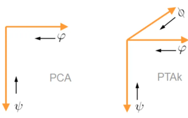
3.2. PTAk-modes of a tensor of order k > 2
Figure 1: Illustrative comparison between PCA and PTAk(here withk= 3) when computing singular values by Complete Contractions given in the Equations 5 and 6: the basis of the
RPVSCC algorithm.
associated with the singular value with the optimization form:
σ1 = max kψks=1 kϕkv=1 kφkt=1 X..(ψ⊗ϕ⊗φ) (6) = X..(ψ1⊗ϕ1⊗φ1)
This is a direct extension of Equation5, as expressed by the practical schemas in Figure1, with contractions made either on a matrix table or on a tensor of order 3. The further extension to
k >3 is straightforward. CONTRACTION.list() is convenient relatively to Equations5 and 6
as it performs the contraction without computing the tensor product of the vectors in the first place as algebraically:
X..(ψ⊗ϕ⊗φ) = (X..ψ)..(ϕ⊗φ) = (X..ϕ)..(ψ⊗φ) = (X..φ)..(ψ⊗ϕ) = ((X..ψ)..ϕ))..φ (7) The functionSINGVA()computes the best rank-one approximation of the given tensorX to-gether with its singular value, given by Equation 6(and a similar equation for higher orders). The therein algorithm, called RPVSCC in Leibovici(1993), is inspired from the algorithm of “reciprocal averaging” (Hill 1973) also known as the “transition formulae” in modern
corre-spondence analysis and in the signal processing community as the “power method”.
Adding an orthogonality constraint to Equation 6allows us to carry on the algorithm to find the second principal tensors and so on. The optimization becomes is equivalent but working on
P(ψ⊥
1⊗ϕ⊥1⊗φ⊥1)X: the orthogonal projection ofXonto the orthogonal tensorial of the principal
tensor,i.e (ψ⊥1 ⊗ϕ⊥1 ⊗φ⊥1); this projector can also be written as (Id−Pψ1)⊗Id−Pϕ1)⊗(Id− Pφ1). Following this algorithm schema, given in Equation8, the PTAk-modes decomposition
obtained offers a way of synthesizing the data according to uncorrelated sets of components. Within this schema implemented for the functions PTA3() and PTAk() one can distinguish main principal tensors from associated principal tensors. The latter are associated with main principal tensors as they show one or more component of this main principal tensor in their sets of components. The associated principal tensors are obtained by a PTA(k−1)-modes decomposition once thek-modes data array has been “contracted” by the given component.
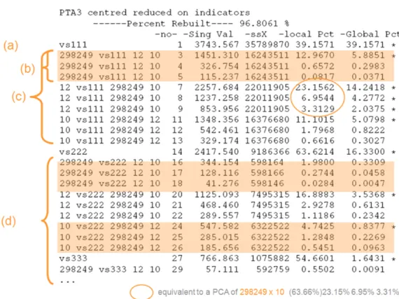
Figure 2: Output summary from the functionsummary()on a “PTAk” object, here the climatic data described in Section 4.3: (a) is the first principal tensor, (c) represents all the associated principal tensors to first one such like (b) are the spatial-mode associated principal tensors, (d) corresponds to a PTAk-modes decomposition of the initial data tensor projected onto the orthogonal tensorial of the first principal tensor.
This makes the algorithm a recursive algorithm with the following procedure, where here
k= 3: PTA3(X) = σ1(ψ1⊗ϕ1⊗φ1) (8) + ψ1⊗1PTA2(P(ϕ⊥1 ⊗φ⊥1)X..ψ1) + ϕ1⊗2PTA2(P(ψ1⊥⊗φ⊥1)X..ϕ1) + φ1⊗3PTA2(P(ψ1⊥⊗ϕ⊥1)X..φ1) + PTA3(P(ψ1⊥⊗ϕ⊥1 ⊗φ⊥1)X)
The notation⊗i means that the vector on the left hand will take theith place, among the k
places here, in each full tensorial product, e.g.,ϕ1⊗2(α⊗β) =α⊗ϕ1⊗β. More details on
the properties of the method and on each function of theRpackage is given in the references
Leibovici and Sabatier(1998);Leibovici (2009).
Equation 8 and Figure 2 illustrate the multi-hierarchical decomposition obtained with the PTAk-modes model. In Figure 2, in almost the same way as for PCA, one gets a hierarchy of principal tensors corresponding to a hierarchy of sum of squares, i.e., by the square of the singular values (σ) under the column -Sing Val associated with each principal tensor. It is a multilevel hierarchy in agreement with Equation8. Percents of variability associated with
each principal tensor can be used to retain the main variability within the data tensor X. These percentages are in the-Global Pctcolumn of Figure2whereas-local Pctare relative to the sum of squares given in column -ssX linked to the current tensorial optimization as defined in Equation 8. Plots of the vector components of a particular principal tensor allows the description of the extracted variability for each principal tensor.
PROJOT()is the function withinPTAk()performing the orthogonal tensor projection of Equa-tion 8but can also be used for any structure or design associated with each mode to perform a linear constrained analysis in the same way as for PCAIV (principal component analysis on instrumental variables), see Leibovici (2000) for a full description of using PTAIVk() and in the PTAkmanual for PROJOT()where a quick implementation is given as an example.
3.3. A brief comparison of multiway models
Before expressing in detail the Rusage of the main methods within PTAk a practical com-parison of the multiway models already described is of use. The models behind the methods
PTAk(),CANDPARA() (PARAFAC/CANDECOMP) andPCAn() (Tucker-nmodel) are equiv-alent when looking for best rank-one approximation. This can be demonstrated from the expression of the models associated with these methods and can be understood from Equa-tions 9and 10. Using an example this would be:
R> library("PTAk")
R> PTAk(X, nbPT = 1, nbPT2 = 0) == CANDPARA(X, dim = 1)
R> PTAk(X, nbPT = 1, nbPT2 = 0) == PCAn(X, dim = rep(1, length(dim(X)))) R> CANDPARA(X, dim = 1) == PCAn(X, dim = rep(1, length(dim(X))))
This cannot be strictly verified using the package PTAk as CANDPARA()and PCAn() in their implementation only accept rank approximation greater than 1. Working around using a tensor “nearly” of rank-one is:
R> X <- c(1, 2, 3) %o% c(2, 4, 6) %o% c(3, 7) + rnorm(18, sd = 0.0001) R> sol1 <- PTAk(X, nbPT = 2, nbPT2 = 0)
R> sol2 <- CANDPARA(X, dim = 2); R> sol3 <- PCAn(X, dim = c(2, 2, 2)) R> sol1[[1]]$v[1, ] [1] 0.2672617 0.5345234 0.8017830 R> sol2[[1]]$v[1, ] [1] -0.2672617 -0.5345234 -0.8017830 R> sol3[[1]]$v[1, ] [1] -0.2672617 -0.5345234 -0.8017830 R> sol1[[3]]$d
[1] 2.132416e+02 2.086484e-04
showing the first mode component for the first principal tensor given by sol1[[1]]$v[1,]
as equal to the other approximations, (it is the same with mode 2 sol[[2]] and mode 3
sol[[3]]). The tensor can be said to be “nearly” of rank-one as the ratio the two singular values, sol1[[3]]$dis 106.
This gives a numerical proof of equivalence between PTAk, PARAFAC/CANDECOMP and
Tucker-n when looking for the best rank-one approximation. Then the methods differ as also differs the rank definition attached to each model. PTAk will try to look for best approximation according to the orthogonal rank, i.e., the rank-one tensors (of the decom-position) are orthogonal; Tucker-n or PCAn-modes will look for best approximation accord-ing to the space-ranks, i.e., ranks of every bilinear form deducted from the original tensor (folding the multi-array into a matrix), that is the number of components in each space; PARAFAC/CANDECOMP will look for best approximation according to the rank, i.e., the rank-one tensors are not necessarily orthogonal.
It is said here “PTAkwilltry” as it has been shown recently on an example that the orthogonal-rank was not necessarily providing a nested decomposition as PTAk-modes implies (Kolda 2003). One can also notice that PTAk model extends the PARAFAC-orthogonal if one only retains in the decomposition the main principal tensors (not the associated ones), i.e., by settingnbPT2 = 0 in thePTAk() call or by ignoring them.
The function REBUILD() will return the approximated or filtered dataset according to the method used, either PTAk(), CANDPARA(), or PCAn(); the parameters of the method are the list of tensors and/or a global threshold for percentage of variability explained by each elementary tensors. For PCAn() the function calls REBUILDPCAn() which does not use these parameters.
R> Xapp <- REBUILD(sol1, nTens = c(1, 2), testvar = 1e-12)
-- Variance Percent rebuilt X at 100 % -- MSE 4.378514e-09
-- with 2 Principal Tensors out of 2 given -- compression 0 %
For PTAk() and CANDPARA(), the approximation is done according to the equation model, here written for a tensor of order 4:
X=X
i∈ς
σiψi⊗ϕi⊗φi⊗ξi+ (9)
where ς is a set of the selected elementary tensors. The PCAn() rebuilt approximation is a direct generalization of model fromKroonenberg and De Leeuw (1980):
X = (Ψ⊗Υ⊗Φ⊗Ξ)..C+ (10)
where the components here are matrices of components with as many columns in each mode-space as asked for during the optimization analysis (the mode-space-ranks), andC being the core
4. Running a general PTA
k
SINGVA(), PROJOT() described above are part of the main functions for 2-modes analysis, such as SVDGen(), and k-modes analysis with PTAk(), CANDPARA() and PCAn(). They can also be used to devise new analysis. So once you have loaded or scanned the dataset from other sources or format, put it in a multi-array, an “array” object inRyou can run thePTAk()
decomposition or the other multiway methods.
4.1. Structure of the PTAk package
The package can be summarized as four series of methods: (i) preprocessing the methods
Multcent(), IterMV(), Detren() for data preprocessing but also some metrics preparation such asCauRuimet(), (ii) the multiway analysis methods PTAk(),FCAk(),CANDPARA(), and
PCAn() which output objects of class “PTAk” and appropriate subclasses given by the name of the analysis along with S3 methods associated with them (iii) plot(), summary(), and
REBUILD(), the other methods (iv) are either internal or used within main methods but they can be used for developing further methods.
The principal argument of the preprocessing methods is an “array” object which has been pre-pared beforehand for data analysis: the array will be the multiway table of the measurements arranged by their modes, i.e., the “dimensions” deserving interest, e.g., time(s), variable(s), subject(s), space(s), countrie(s), or condition(s). Whichever name used to describe an entry of the table, it has a particular semantic according to the study. For example time for the ecolimatic study example corresponds to 12 months, and for the pharmaco-dynamic study it is the hour and minutes at measurements. Some examples of preprocessing are given in Section4.3, see the help files of the package for a detailed description of the other arguments. The principal arguments for the analysis methods are first of all, either an “array” object of the multiway dataset or a “list” object with $dat containing an “array” object and $met
containing the metrics associated with each entry of the array, then the “amount” of approx-imation chosen. A metric is a semi-definite positive symmetric matrix allowing to perform non-canonical scalar product, i.e., covariance, “sum of squares of products”, within the cor-responding vectorial space (see Section6 for further explanation). The arguments related to this “amount” of approximation chosen are: dim an integer for CANDPARA() and a “vector” object of integers forPCAn()fixing respectively as described previously the number of elemen-tary tensors to fit, and the size of the core tensor (therefore the number components in each space); for PTAk() one chooses the number of principal tensors at each “level” of analysis by
nbPT, the last level (2-modes analysis) is fixed by nbPT2. Note that for PTA3-modes() nbPT
has to be just an integer but fork >3 it can be a vector (of length (k−2)) specifying this choice for each level above 2-modes analysis. The current version of the package doesn’t give much support for other plots or interpretations for CANDPARA() and PCAn(). For example the summary() method on a PCAn object doesn’t properly describe the core tensor and no jointplot method (see Kroonenberg 1983) has been implemented yet in the package PTAk. Further practical use of the functions are described in the help files of the packageLeibovici
(2009), but some practical examples are given in the next section.
4.2. Practical example
Lei-boviciet al.2007), where dynamics over a typical year of 10 climatic indicators were analysed in the circum-saharan zone, using their monthly average estimates. The problematic explained inLeiboviciet al.(2007) is to delineate homogeneous zones in relation to the ecolimatic profile (rainfall, temperature, evapotranspiration, etc.). So finding main spatial patterns via the spa-tial components associated with a climatic profile and a seasonal pattern, was the aim of this analysis. Here the studied zone has been limited to Tunisia; the shapefile contains a regular grid with the multivariate values. The dataset Zone_climTUN was obtained using the call
read.shape("E:/R_GIS/R_GilHF/TUN/tunisie_climat.shp") based on the read.shape()
function from the MAPS package. For replication, the data are also available in PTAk:
R> library("PTAk") R> library("maptools") R> data("Zone_climTUN")
The next command produces a plot of a MAPobject not shown here:
R> plot(Zone_climTUN, ol = NA, auxvar = Zone_climTUN$att.data$PREC_OCTO,
+ nclass = 20)
The data are transformed into an arrayobject:
R> Zone_clim <- Zone_climTUN$att.data[, c(2:13, 15:26, 28:39, 42:53,
+ 57:80, 83:95, 55:56)]
R> Zot <- Zone_clim[, 85:87] R> temp <-colnames(Zot)
R> Zot <- as.matrix(Zot) %x% t(as.matrix(rep(1, 12))) R> colnames(Zot) <- c(paste(rep(temp [1], 12), 1:12),
+ paste(rep(temp [2], 12), 1:12), paste(rep(temp [3], 12), 1:12))
R> Zone_clim <- cbind(Zone_clim[, 1:84], Zot) R> dim(Zone_clim)
[1] 2599 120
R> Zone3w <- array(as.vector(as.matrix(Zone_clim)), c(2599, 12, 10)) R> dim(Zone3w)
[1] 2599 12 10
R> dimnames(Zone3w) <- list(rownames(Zone3w), 1:12, c("P", "Tave", "ETo", + "PETo", "Tmax", "Tmin", "Q3", "Alt", "dM2T", "dMETo"))
R> Zone3w.PTA3-modes <- PTA3-modes(Zone3w, nbPT = 3, nbPT2 = 3, + minpct = 0.1, addedcomment="centr´ee r´eduite sur var")
---Final iteration--- 7
--Singular Value-- 59898.86 -- Local Percent -- 97.62936 % ---Final iteration--- 26
---Final iteration--- 39
--Singular Value-- 401.1593 -- Local Percent -- 38.09571 % ++ Last 3-modes vs < 0.1 % stopping this level and under ++ ---Execution Time--- 7.43
R> summary(Zone3w.PTA3-modes, testvar = 0.01)
++++ PTA3-modes ++++
data = Zone3w 2599 12 10 PTA3-modes centr´ee r´eduite sur var
---Percent Rebuilt---- 99.97716 %
---Percent Rebuilt from Selected ---- 99.95512 %
-no- --Sing Val-- --ssX-- --local --Global Pct--vs111 1 59898.9 3674994157 97.62936 97.629361 2599 vs111 12 10 3 3243.0 3598688392 0.29226 0.286187 12 vs111 2599 10 6 7354.4 3652184965 1.48097 1.471774 12 vs111 2599 10 7 3142.0 3652184965 0.27031 0.268629 vs222 11 2860.4 11915003 68.66842 0.222636 12 vs222 2599 10 16 1677.1 11037709 25.48250 0.076536 ++++ ++++
Shown are selected over 15 PT with var> 0.01 % total
The first principal tensor captures most of the variability, 97.6%, nearly as much as the decomposition up to 3 main principal tensors and 3 for each associated, i.e., at each second level analysis (a PCA). Notice that the listing should be 30 lines long, as for each main principal tensor, 9 associated principal tensors are requested (nbPT2 = 3), but redundant tensors are removed automatically and out of the 21 potential principal tensors a selection has been performed here: Global Pct> 0.01%. The listingsummary() mentions “...over 15 PT” as in the call function, the parameter minpct = 0.1 forces the algorithm to stop a
k≥3-level (no sub-level analysis), if this percentage of variability is not met: it was the case here for vs333. The full description of the ouput summary() is explained in the Section4.4
where the listing ouput provides a more complete form.
This first PTAk analysis is not very useful as the variations and range of values can be very different from one climatic variable to another. So the main variations captured by the principal tensors will be towards this differentiation without necessarily expressing the interactions between the variables and them with the spatio-temporal domain which may only be detected in some principal tensors (main or associated) with comparatively small singular values. As for PCA, centering and scaling the variables, preprocessing transformation may be crucial as part of the modelling and analysis process.
4.3. Array data and preprocessing
In the ecoclimatic data example the variables of interest are in mode 3, the climatic indicators, as the other tow modes are their support, the spatial-locations and the months. How does one center and scale the 10 indicators? It depends on the variability of the data one put the focus on, so this has to be considered as a part of the model. Here we are focusing on the
spatio-temporal dynamics of the indicators, so we are looking for spatial patterns and tempo-ral patterns of the correlations of the variables. For a given spatial-location or spatial trend one would like to detect the mean temporal patterns of evolution or seasonality, therefore it is not desirable to center and scale the indicators for each month over the spatial-locations. It is also desirable to detect spatial mean patterns for a given month or temporal trend. There-fore, centering and scaling the indicators along the whole spatio-temporal observations seems appropriate. This would be the transformation to do, to perform a PCA on the indicators with spatial observations repeated over the 12 months.
Another interesting preprocessing would have been to perform a bi-centering along spatial-location and month modes for each indicator in order to emphasize only on interactions but not on marginal effects.
Performing centering and scaling can be done with the function Multcent() which proposes a centering and/or a scaling along the by mode(s) combination, before and/or after, xxxBA
some possible “multi-centering” along each bi combined withby. For example a bi-centering on a three-way table corresponding to an ANOVA way of removing each of the two first factor effects and the mean effect for each level of the third factor can be done with:
R> Zone3w.bi <- Multcent(dat = Zone3w, bi = c(1, 2), by = 3, centre = mean,
+ centrebyBA = c(FALSE, FALSE), scalebyBA = c(FALSE, FALSE))
More advanced centering and scaling can be used iteratively with IterMV() as each trans-formation may destroy the other one, but one could possibly reach convergence in this pre-modeling step. For example removing a smooth trend of the months and scaling spatially the results would be:
R> Zone3w.DS <- IterMV(n = 10, dat = Zone3w, Mm = c(1, 3), Vm = c(2, 3),
+ usetren = TRUE, tren = function(x) smooth.spline(as.vector(x),
+ df = 5)$y, rsd = TRUE)
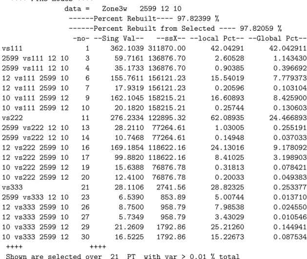
Simple centering and scaling as mentioned before has been performed for the ecoclimatic data for Tunisia. This allows us to extract spatio-temporal trends and spatio-temporal interactions with the indicator mode.
R> Zone3w <- Multcent(dat = Zone3w, bi = NULL, by = 3, centre = mean,
+ centrebyBA = c(TRUE, FALSE), scalebyBA = c(TRUE, FALSE))
R> Zone3w.PTA3-modes <- PTA3-modes(Zone3w, nbPT = 3, nbPT2 = 3)
---Final iteration--- 37
--Singular Value-- 362.1039 -- Local Percent -- 42.04291 % ---Final iteration--- 25
--Singular Value-- 276.2334 -- Local Percent -- 62.08935 % ---Final iteration--- 56
--Singular Value-- 28.11064 -- Local Percent -- 28.82325 % ---Execution Time--- 9.57
++++ PTA3-modes ++++
data = Zone3w 2599 12 10
---Percent Rebuilt---- 97.82399 %
---Percent Rebuilt from Selected ---- 97.82059 %
-no- --Sing Val-- --ssX-- --local --Global Pct--vs111 1 362.1039 311870.00 42.04291 42.042911 2599 vs111 12 10 3 59.7161 136876.70 2.60528 1.143430 2599 vs111 12 10 4 35.1733 136876.70 0.90385 0.396692 12 vs111 2599 10 6 155.7611 156121.23 15.54019 7.779373 12 vs111 2599 10 7 17.9319 156121.23 0.20596 0.103104 10 vs111 2599 12 9 162.1045 158215.21 16.60893 8.425900 10 vs111 2599 12 10 20.1820 158215.21 0.25744 0.130603 vs222 11 276.2334 122895.32 62.08935 24.466893 2599 vs222 12 10 13 28.2110 77264.61 1.03005 0.255191 2599 vs222 12 10 14 10.7468 77264.61 0.14948 0.037033 12 vs222 2599 10 16 169.1854 118622.16 24.13016 9.178092 12 vs222 2599 10 17 99.8820 118622.16 8.41025 3.198903 10 vs222 2599 12 19 15.6388 76876.78 0.31813 0.078421 10 vs222 2599 12 20 12.4100 76876.78 0.20033 0.049383 vs333 21 28.1106 2741.56 28.82325 0.253377 2599 vs333 12 10 23 6.5390 853.89 5.00744 0.013710 12 vs333 2599 10 26 8.7500 958.79 7.98538 0.024550 12 vs333 2599 10 27 5.7349 958.79 3.43029 0.010546 10 vs333 2599 12 29 21.2609 1792.86 25.21260 0.144941 10 vs333 2599 12 30 16.5225 1792.86 15.22673 0.087534 ++++ ++++
Shown are selected over 21 PT with var > 0.01 % total
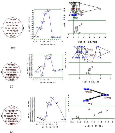
Some other preprocessing transformations or pre-model examples can be seen with the EEG data in Leibovici (2000), exploiting the ANOVA interpretation of the factors involved. The EEG data consisted of a repeated cross-over design on 12 subjects with 3verum doses (10mg, 30mg and 90mg) and 1 placebo. The EEG bands quantification was available spatially at 28 electrodes with repetitions over 10 times of measurements (before drug administration and every hour or so after until 6 hours post-dosing). For this dataset the preprocessing aim was pretty much towards minimizing subject variability. Part of Figure 4 in Leibovici (2000) is reproduced here in Figure3, showing a comparison of the first principal tensors obtained from PTA4-modes of thesubject×dose×electrode×time×EEG−band with different centering and scaling. So the best result (c) was obtained after scaling each subject and then removing the subject effect and all two-way interactions with the subject factor. Would it have been better to remove subject 11 from the analysis?
4.4. Summary method on “PTAk” objects
Figure 2 and the previous output are examples of output from the summary() method of “PTAk” objects generated by calling PTAk() and the other methods in the R package. The identifier for singular values and principal tensors corresponds to the column-no-which is the order number in the processing history. The first column of the output table fromsummary()
Figure 3: 1st principal tensor from PTA4-modes of the EEG data versus baseline versus
placebo with different centering and scaling: (a) raw data, (b) subject scaled, (c) ANOVA residuals from subject factor (main effect and other two-ways interactions with it) —the subject— doses and bands plots are artificially scattered vertically for better reading of the dispersion on the horizontal axe (means by dose have been overlaid).
qualifies the identifier with a leading name. For main principal tensors the name is unique, like vs111 orvs222 where the number corresponds to an order from the top level hierarchy (the repetition of the number is to emphasize the level of the hierarchy corresponding to the order of the current tensor analyzed). The others names are qualifying associated principal tensors, expressing the dimension of the mode from which the association is made (contraction by the corresponding component vector). In 3-modes analysis, they also show the last two dimensions (on which a PCA is done).
For PTA4-modes the schema starts with vs1111, the second level corresponds to 3-modes analyses with names such as 12-vs222 where here the component contracting the data is explicit for the dimension, 12, but implicit for the principal tensor it comes from, as here
vs222expresses the current 3-modes analysis. The third level brings in names such as12-300 vs222 10 7 with the same meaning as in 3-modes analysis: associated with the PCA on the table 10×7. This schema is then similar for all other higher modes. Notice for the
4-modes analysis there is no12-vs111as in fact thisSINGVA()optimization is redundant with the vs1111 solution. In the same manner, the first principal component for every 2-modes analysis is redundant with the solution just optimized within the 3-modes analysis. This comes from the fact that in order to really take the benefit of the recursivity it is easier in the implementation of Equation 8 to perform the PTA(k−1)-modes analysis just onto the contracted tensor and not onto the projection of it on the tensorial orthogonal of the rest of the principal tensor. Computationally it is then easier to let the recursive algorithm perform all the solutions associated and discarding the redundant ones. That is why there are gaps in the number for the column-no-, e.g., after the principal tensor-no- 1 there will never be a principal tensor-no- 2. The generic form of the PTAk() algorithm which is implemented in theRpackage is then:
PTAk(X) = σ1(ψ11⊗ψ12⊗...⊗ψ1k) (11) + ψ11⊗1PTA(k−1)∗(X..ψ11) + ψ21⊗2PTA(k−1)∗(X..ψ12) + ... + ψk1 ⊗kPTA(k−1)∗(X..ψ1k) + PTAk(P(ψ11⊥⊗ψ12⊥⊗...⊗ψk1⊥)X)
in where∗ means that the “top” solutions of each PTA(k−1)-modes have to be discarded as redundant from previous optimization.
5. Plotting and interpreting
A class “PTAk” object is a list of lists. For each mode of the tensor, the list, reachable by its mode number in the dimension of the array, contains few descriptors of the mode and the components stored in a matrix$vwhere the row numbers match the order (-no-) given in the
summary(), while the columns are the names list given in$n (taken from the dimnames()of the array) for the corresponding mode. The list for last mode has extra summaries describing the analysis (applicable to all modes or the whole analysis), such as the singular values stored in$d: R> Zone3w.PTA3[[3]]$v[c(1, 9, 11), ] [,1] [,2] [,3] [,4] [,5] [,6] [1,] 0.2406405 -0.4552913 -0.4382538 0.2727417 -0.4560138 -0.4447370 [2,] 0.2406405 -0.4552913 -0.4382538 0.2727417 -0.4560138 -0.4447370 [3,] -0.2976787 -0.1066016 -0.0960886 -0.1850355 -0.1017793 -0.1103574 [,7] [,8] [,9] [,10] [1,] 0.2501758 0.001285919 -0.003664209 -0.002239094 [2,] 0.2501758 0.001285919 -0.003664209 -0.002239094 [3,] -0.2404791 -0.297859857 0.610534012 0.560992015 R> Zone3w.PTA3[[3]]$d[c(1, 9, 11)] [1] 362.1039 162.1045 276.2334
R> Zone3w.PTA3[[3]]$n
[1] "P" "Tave" "ETo" "PETo" "Tmax" "Tmin" "Q3" "Alt" "dM2T" "dMETo"
Notice that here, looking at the components for mode 3 of the tensors 1, 9, and 11, the principal tensor 9 is an associated principal tensor to the first principal tensor via the indicator mode, its component for this mode is therefore equal to the one from the first principal tensor. Interpretations of the extracted features of the dataset expressed in the principal tensors can be derived from various plots of components which can be read simultaneously. For the ecocli-matic analysis one would read and interpret a map configuration (spatial-locationcomponent), an annual pattern (month component) and an axis describing associations and oppositions of the variables (indicator component), together expressing the monthly dynamic of the eco-climatic characteristics. PTAkprovides a plot() method for “PTAk” objects which basically overlays the scattering plots of components for the asked modes. For the spatial component here we used a modified version of theplot.Map()(given in the file “v34i10-additions.R”). The followingplot() calls can be seen on Figure4 which gathers the basic 3 plots related to the principal tensors 1 and 11: the first plot is a joint plot of their modes 2 and 3 (time and indicators), the other plots are their respective spatial modes (mode 1).
R> plot(Zone3w.PTA3-modes, mod = c(2, 3), nb1 = 1, nb2 = 11,
+ lengthlabels = 5, coefi = list(c(1, 1, 1), c(1, -1, -1)))
R> plot(Zone_climTUN, ol = NA, auxvar = Zone3w.PTA3-modes[[1]]$v[1, ],
+ nclass = 30, colrmp = colorRampPalette(Yl)(31), mult = 100)
R> plot(Zone_climTUN, ol = NA, auxvar = Zone3w.PTA3-modes[[1]]$v[11, ],
+ nclass = 30, colrmp = colorRampPalette(Yl)(31), mult = 100)
Looking closely at the given outputs, one sees that the principal tensor-no- 11,vs222, makes an opposition between “number of dry months”dM2T,dMETo(two different ways deriving this ecoclimatic indicator) with positive weightings and the other indicators with negative weights. Nonetheless the plot() on Figure 4 shows the opposite signs and as a matter of fact the argument coefi, in the call of theplot(), is indicating this change for the tensornb2 = 11
on mode 2 and 3. The reason for this ad-hoc change can be understood for example from the fact:
ψi⊗ϕi⊗φi⊗ξi=ψi⊗(−ϕi)⊗φi⊗(−ξi) (12) So as in PCA where a principal component and the corresponding variable loadings can be arbitrarily multiplied by (−1),k-modes analysis havingk >2 set of components will show dif-ferent ways of distributing this changes. Therefore simultaneous or joint interpretation has to be cautious about this fact. Interpretation has to look at either components separately giving a within-component description (association, opposition, etc.) or all the component scores giving a whole principal tensor interpretation, but not reading only 2 out of 3 components for example.
Using the associativity of the tensor product, a theoretical example of reading associations and oppositions for different components is given in Table1, the interpretations are all compatible, and also identical for any other tensor equivalence transformation.
In PCA, examining correlations of variables with the principal components is the traditional way of having interpretations across components. The duality in 2-modes analysis implies
Figure 4: Principal tensors 1 and 11 from PTA3-modes of the ecoclimatic Tunisian data. − + ψ A B ϕ t1 t2 φ n m ψ ⊗ ϕ ⊗ φ ψ ⊗ (−ϕ) ⊗ (−φ) (−ψ) ⊗ ϕ ⊗ (−φ) (−ψ) ⊗ (−ϕ) ⊗ φ Oppositions 2 by 2 (Bt2m) , (At1m), (Bt1n), (At2n)
Table 1: Linked information: Tensor Components | Tensor Equivalences | Interpretations across components: (xyz) meaning semantic association.
full equivalence as reading interpreting directly the factor loadings. With 3-modes, theses correlations have to be between the variables represented by the vectors of the tensor unfolded into a matrix and the ψi ⊗φi (for the 2-modes variables). Similar considerations occur with
6. PTA
k
-modes with non identity metrics
As mentioned in the introduction, all multiway decomposition methods in PTAk allow us to use non-identity metrics for every space involved in the tensorial space, i.e., symmetric positive definite matrices used in the inner products within each space. (The canonical inner product —sum of cross-products— corresponds to the identity metric and the metric on the tensorial space the tensorial product of the individual metrics, see for exampleLeibovici 1993;
Dauxoiset al.1994). Instead of feeding the methods with an “array” objectX, one uses alist
where$datacontains the “array” object and$metis a listof “matrix” objects or “vector” object objects (diagonal metrics) representing the metrics associated with the inner products in each space. Algebraically within the tensor framework this has an effect on the contracted product and on the norms of the vectors, therefore on the optimization of Equations6 and its equivalent for anyk. Going back to one of the definitions of the tensorial product gives a hint for this natural extension:
ha⊗b⊗c, ψ⊗ϕ⊗φiD⊗Q⊗M =ha, ψiDhb, ϕiQhc, φiM = taDψtbQϕtcM φ (13)
whereaand ψ belong to the metric space Rs with as metric the symmetric positive definite
matrix D, s being the length of vector a, and similar definitions for the other elements of Equation 13. If a, b, and c cover the canonical basis elements in each space and X being expressed naturally in this basis, it is possible to grasp via the contraction of elementary tensors (rank one tensors), the utilisation of metrics in the contraction of any two tensors. Computationally one could also write:
X..m(ψ⊗ϕ⊗φ) = t(t(tXDDψ)QQϕ)MM φ (14)
in which the use of non-identity metrics in the contracted product has been emphasized by a subscript..m; the subscript with a metric means rearranging the given tensor in a matrix where the columns lie in that metric space, i.e., the number of rows is equal to the dimension of the given metric space.
Like in PCA or SVD, where one analyses a triplet (X, Q, D), data and metrics for the two modes, it is convenient to refer to (k+ 1)-uples of objects defining the analysis, that is the tensor of orderk as the data, and thek metrics associated to each mode of the tensor:
(X, M1, M2, ..., Mk) (15)
6.1. Use of metrics in PCA
A PCA of a triplet (X, Q, D) withX a data matrix n×p,Q ap×p metric on the rows (or in the column-space) and similarly D a n×n metric on the columns (or in the row-space), is generalizing a standard PCA by diagonalizing withQ-normed vectors the matrix tXDXQ
equivalent, to the covariance matrix ifX is column-centered, D= 1/nIdn andQ= Idp, or to
the correlation matrix if instead of the identity metric Q = diag(1/var1. . .1/varp) (see also Dray and Dufour 2007, for more details).
6.2. Choice of metrics for spatial data
A classical use of metrics is in discriminant analysis when a known group structure is part of the design experiment, and either assessing or minimizing the impact of this structure on
the variability is the goal of the analysis. For example it would be possible to a perform (i) a PTAIVk-modes to assess the known structure and (ii) an orthogonal-PTAIVk-modes (that is a residual analysis) to minimize the structure in the analysis, where using as metric the inverse of within-group variations would improve both analyses. When the structure is unknown, as is often the case, the goal of the analysis becomes to look for what is structuring the data. As mentioned by Caussinus and Ruiz (1990) a good strategy to reveal dense groups with generalized PCA would be to reveal outliers first using the metricWo−1 given in Equation 17
with 0.05 ≤ β ≤ 0.03 and remove them before using the metricWl−1, Equation 16, using a
β ≥ 1. Wl is a robust estimate of the within covariance of the unknown structure given by
the functionCauRuimet:
Wl =
Pn−1
i=1
Pn
j=i+1Gijker(d2S−(Zi, Zj))(Zi−Zj)t(Zi−Zj)
Pn−1
i=1
Pn
j=i+1Gijker(d2S−(Zi, Zj))
(16)
where Z is a data matrix, d2S−(., .) is the squared Euclidean distance with S− the inverse
of a robust sample covariance andG is a graph structure expressing some known proximity (when no knowledge of proximity is chosen Gij = 1 and one just has to put mo = 1 in the
function). ker is a positive decreasing function which would provide a kernel function for the different weighting: by default e−βu with choices on β. Wl corresponds to the definition of local variance (Lebart 1969;Caussinus and Ruiz 1990;Faraj 1994).
Wo=
Pn
i=1ker(d2S−(Zi,Z˜))(Zi−Z˜)t(Zi−Z˜)
Pn
i=1ker(d2S−(Zi,Z˜))
(17) To complete the different metrics or semi-metrics associated to known or unknown structure variances, the function can give also something analog to a global variance:
Wg =
Pn−1
i=1
Pn
j=i+1Gijker(d2S−(Zi, Zj))(Zi−Z˜)t(Zj−Z˜)
Pn−1
i=1
Pn
j=i+1Gijker(d2S−(Zi, Zj))
(18)
where ˜Z is the location vector of the multivariate distribution, i.e., a robust estimate of the mean. In the case of some known structure the semi-metricWlgα−=Wg1/αWl−1W g1/αmay be
used to extract robust sub-structure, in the sense that the analysis will tend to minimize the local variance and be consistent at 1/α with the global variance, with convergence towards
Wl−1 asα increases.
So far, using these metrics is not specific to spatial data as even the graph structure can reflect any proximity in attribute space, but it is also reminiscent of neighborhood graphs as inLebart (1969); Faraj (1994). In a spatial context, Wlgα− is particularly interesting when looking for finer-scale structures compatible with some coarser scale relationships represented by theGij (Gtaken into account inWg but in Wl computations).
With the Tunisian climatic data example, we used Wly−1 as metric in the indicators space
computed on the yearly average across spatial-location but also the same metric computed on the concatenated array across spatial-location and month mode (noted belowWl−1).
R> Zvm <- CONTRACTION(Zone3w, rep(1/12, 12), Xwiz = 2, zwiX = 1) R> Wly <- CauRuimet(Zvm, ker = 2, m0 = 1, withingroup = TRUE,
R> Wlv <- Powmat(Wly, -1)
R> Zone3w <- list("data" = Zone3w, "met" = list(1, 1, Wlv))
R> Zone3w.PTA3-modesm3 <- PTA3-modes(Zone3w, nbPT = 3, nbPT2 = 3, + modesnam = c("carte", "mois", "var"),
+ addedcomment = "PTA3-modes metric Wly var yearly")
R> summary(Zone3w.PTA3-modesm3, testvar = 1e-2)
++++ PTA3-modes ++++
PTA3-modes metric Wly var yearly data = Zone3w 2599 12 10 ---Percent Rebuilt---- 96.56307 %
---Percent Rebuilt from Selected ---- 96.46785 % -no- --Sing Val-- --ssX-- --local --Global Pct--vs111 1 801.918 1112488.0 57.8049 57.80492+ 2599 vs111 12 10 3 308.729 750707.7 12.6965 8.56761+ 2599 vs111 12 10 4 104.273 750707.7 1.4483 0.97734 12 vs111 2599 10 6 404.862 821714.2 19.9477 14.73391+ 12 vs111 2599 10 7 101.507 821714.2 1.2539 0.92618 10 vs111 2599 12 9 100.671 658692.8 1.5386 0.91099 10 vs111 2599 12 10 51.986 658692.8 0.4103 0.24293 vs222 11 287.342 167518.8 49.2871 7.42167-2599 vs222 12 10 13 138.938 102851.1 18.7685 1.73518 ...
The summary description of the analysis shows a “concentration” of explained variability onto the first principal tensors (marked with a +) with a decrease for example of vs222. Nonethe-less usingWly−1, little differences were seen for the spatial components. When using theWl−1
metric instead, taking into accountmonth differences, results are completely redistributed in the principal tensors as for example the principal tensorvs222of the analysis without metric now becomes the main features extracted by vs111, see and compare Figures 5and 4.
R> Zv <- matrix(as.vector(aperm(Zone3w$data, c(1, 2, 3))), c(2599*12, 10)) R> Wlv <- Powmat(CauRuimet(Zv, ker = 1, m0 = 1, withingroup = TRUE,
+ loc = substitute(apply(Z, 2, mean, trim = 0.1)),
+ matrixmethod = TRUE), -1)
R> Zone3w.PTA3-modesm3all <- PTA3-modes(list("data" = Zone3w$data, + "met" = list(1, 1, Wlv)),
+ nbPT = 3, nbPT2 = 3, modesnam = c("carte", "mois", "var"),
+ addedcomment = "PTA3-modes metric Wlv var")
R> summary(Zone3w.PTA3-modesm3all, testvar = 1e-2)
++++ PTA3-modes ++++
PTA3-modes metric Wlv var data = Zone3w 2599 12 10 ---Percent Rebuilt---- 82.45044 %
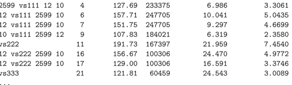
---Percent Rebuilt from Selected ---- 79.82162 % -no- --Sing Val-- --ssX-- --local --Global Pct--vs111 1 411.92 493139 34.408 34.4080 2599 vs111 12 10 3 210.18 233375 18.929 8.9582
2599 vs111 12 10 4 127.69 233375 6.986 3.3061 12 vs111 2599 10 6 157.71 247705 10.041 5.0435 12 vs111 2599 10 7 151.75 247705 9.297 4.6699 10 vs111 2599 12 9 107.83 184021 6.319 2.3580 vs222 11 191.73 167397 21.959 7.4540 12 vs222 2599 10 16 156.67 100306 24.470 4.9772 12 vs222 2599 10 17 129.00 100306 16.591 3.3746 vs333 21 121.81 60459 24.543 3.0089 ...
Figure 5 is realised from the three different plots given below, the scatter plot being done using theplot.PTAk()method, and spatial components plotted using plot.Map() from the
maptoolsRpackage:
R> plot(Zone3w.PTA3-modesm3all, mod = c(2, 3), nb1 = 1, nb2 = 11,
+ lengthlabels = 5)
R> plot(Zone_climTUN, ol = NA, auxvar = Zone3w.PTA3-modesm3all[[1]]$v[1, ],
+ nclass = 30, colrmp = colorRampPalette(Yl)(31), mult = 100)
R> plot(Zone_climTUN, ol = NA, auxvar = Zone3w.PTA3-modesm3all[[1]]$v[11, ],
+ nclass = 30, colrmp = colorRampPalette(Yl)(31), mult = 100)
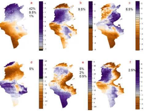
Now using this metric combining smoothed global variance constraint with inverse within local structure, given byWlgα−, the results demonstrate a more interesting spatial pattern than in previous analysis, Figure6. Note as in the analysis withWl−1,vs222of the previous analysis (without metric) now becomes the main features extracted byvs111, elsewhere different in a compatible description of the spatio-temporal patterns as expected by the link between the metrics.
R> DD <- round(100*t(Zone3w.PTA3-modes[[1]]$v[c(1, 6, 9, 11, 16, 17), ]))
R> ddd2 <- exp(as.matrix(round(dist(DD)))) R> ddd2 <- 1/(1 + (ddd2-min(ddd2)))
R> ddd2[ddd2 <= quantile(ddd2, probs = 0.25)] <- 0
R> Zv1 <- CONTRACTION(Zone3w$data, rep(1, 12), zwiX = 1, Xwiz = 2) R> Wov <- CauRuimet(Zv1, ker = 2, m0 = ddd2, withingroup = FALSE,
+ loc = substitute(apply(Z, 2, mean, trim = 0.1)), matrixmethod = FALSE)
R> Wglv <- Powmat(Wov, 1/9) %*% Wlv %*% Powmat(Wov, 1/9)
R> Zone3wgl.PTA3-modes <- PTA3-modes(list("data" = Zone3w$data,
+ "met" = list(1, 1, Wglv)), nbPT = 3, nbPT2 = 3,
+ modesnam = c("carte", "mois","var"),
+ addedcomment = "PTA3-modes metric Wglv")
R> summary(Zone3wgl.PTA3-modes, testvar = 1e-2)
++++ PTA3-modes ++++
data = list(data = Zone3w$data, met = list(1, 1, Wglv)) 2599 12 10 PTA3-modes metric Wglv
---Percent Rebuilt---- 87.57398 %
Figure 5: Principal tensor 1 and 11 (vs111and vs222)) using Wl−1 metric for the indicator mode.
-no- --Sing Val-- --ssX-- --local --Global Pct--vs111 1 1233.432 3609793 42.14520 42.145198 a 2599 vs111 12 10 3 590.828 1913730 18.24071 9.670305 a 2599 vs111 12 10 4 194.028 1913730 1.96720 1.042910 a 12 vs111 2599 10 6 584.066 2348657 14.52462 9.450226 b 12 vs111 2599 10 7 480.787 2348657 9.84207 6.403597 c 10 vs111 2599 12 9 429.092 1731332 10.63456 5.100556 d 10 vs111 2599 12 10 97.945 1731332 0.55409 0.265754
Figure 6: Main spatial components from principal tensors of Tunisian climatic data with metricWlgα−: letters correspond to the output listing with (metric Wglv).
vs222 11 412.755 658783 25.86084 4.719574 e 2599 vs222 12 10 13 265.521 267878 26.31853 1.953064 e 2599 vs222 12 10 14 150.321 267878 8.43528 0.625971 e 12 vs222 2599 10 16 295.822 370631 23.61118 2.424251 f ...
The coarse structure, used here for the Wlgα− metric, is a non-linear transformation of dis-tances (see ddd2 in the above code chunk) based on components extracted from the PTA3-modes without metric (from which global spatial effects were expected to emerge). This par-ticular example, with this choice of coarse structure, could be seen as as an iterative process, assimilating non-linear estimation of smoothed spatial pattern, from and within constrained spatio-temporal decomposition of multivariate dynamics.
In a similar context, geographically weighted discriminant analysis (Brunsdon et al. 2007), takes a similar kernel approach with geographic distances, to take into account spatial prox-imity in the estimation of variance-covariance matrix playing also the role of a metric. The approach ofBorcard and Legendre (2002), claiming to account for a range of scales by using an eigenvalue decomposition of a truncated matrix of distances between sampling sites, is also applicable here to build a metric depending on spatial proximity.
7. Correspondence Analysis on
k
-way tables
The tensorial framework developed previously, using different metrics and particular datasets to perform a PTAk-modes, extends the framework of multidimensional analysis using PCA as a generic method (Escoufier 1987;Dray and Dufour 2007). A method of particular interest is
correspondence analysis; a generalization to multiple contingency table (Leibovici 1993,2000), has been used to analyze spatial patterns of attributes of categorical variables (Leiboviciet al.
2008).
7.1. 2-way correspondence analysis
Correspondence analysis (FCA) of a two-way contingency table with cells nij, i = 1, . . . , I,
j= 1, . . . , J can be described as follows. The usual notations are:
ni.=X j nij, n.j=X i nij, n..=N =X ij nij
and then the observed proportions are defined as pij =nij/N. Diagonal metrics containing
vector margins PI.= t(· · ·pi.· · ·) and P.J used thereafter, are notedDI and DJ. Correspon-dence analysis provides a decomposition of the measure of lack of indepenCorrespon-dence between the two categorical variables indexed respectively by iand j in performing the principal compo-nent analysis, PCA or generalized PCA, of the following triplet (Escoufier 1987):
(DI−1P D−J1 DI, DJ) (19)
The measure of lack of independence is linked to the analysis by: 1 +χ 2 N = 1 + X ij (pij−pi.p.j)2 pi.p.j = X ij pi.p.j( pij pi.p.j) 2 =X s σ2s (20)
where theσs are the singular values from the PCA of the triplet given which hasσ0 = 1 with
components equal to unit vectors in their respective spaces.
7.2. k-way correspondence analysis
As FCA is a particular PCA, we proposed a generalization of correspondence analysis to k -way tables, FCAk-modes, as particular PTAk-modes (Leibovici 1993). Presenting here only the case k = 3, and using similar notations as in the previous section, the three-way table
I×J×K, is analyzed by the PTA3-modes of the quadruple:
((DI−1⊗DJ−1⊗DK−1)..P, DI, DJ, DK) (21)
If one notes: Πijk = Π.jk+ Πi.k + Πij.+ ∆ijk for
(pijk−pi..p.j.p..k pi..p.j.p..k ) = (p.jk−p.j.p..k p.j.p..k ) + (pi.k−pi..p..k pi..p..k ) + (pij.−pi..p.j. pi..p.j. ) + (pijk−δijk pi..p.j.p..k ),
where δijk=pij.p..k+pi.kp.j.+p.jkpi..−2pi..p.j.p..k, one has the following property:
kΠijkk2=kΠ.jkk2+kΠi.kk2+kΠij.k2+k∆ijkk2 (22)
where k.k is the norm on the tensor space, i.e., using the metric DI ⊗DJ ⊗DK. This
re-sult dates from Lancaster in 1951, reported more recently in Carlier and Kroonenberg(1996) where another generalization of correspondence analysis is derived. Equation 22 means that deviation from three-way independence can be orthogonally decomposed into deviations from
independence for the two-way margins of the three-way table, and a three-way interaction term. Each two-way margin deviation from independence is reminiscent of (simple) corre-spondence analysis:
χ2
N =
X
ijk
pi..p.j.p..k(pijk−pi..p.j.p..k
pi..p.j.p..k )2 (23) = X jk p.j.p..k(p.jk−p.j.p..k p.j.p..k ) 2+X ik
pi..p..k(pi.k−pi..p..k
pi..p..k )
2+X
ij
pi..p.j.(pij.−pi..p.j.
pi..p.j. ) 2 + X ijk pi..p.j.p..k( pijk−δijk pi..p.j.p..k )2.
showing that, the PTA3-modes (Equation21) simply retrieves the two-way lacks of marginal independence, and this, in a natural way according to the algorithm schema11. The inertia or sum of squares is:
X ijk pi..p.j.p..k( pijk pi..p.j.p..k )2 = r X s=0 σs= 1 + r X s=1 σs= 1 + χ 2 N (24)
where the first (s = 0) principal tensor being 1II ⊗1IJ ⊗1IK with σ0 = 1, its associated principal tensors relate to two-way margins decompositions, i.e., each term of the second row of the Equation 23. The use of the FCAk() function, implementing this particularPTAk(), is described in the next section for a particular spatial analysis.
7.3. Analyzing multiple collocations
Looking at collocations of attributes with v ≥ 1 categorical variables issued from spatial-location processes (such as point processes) leads to analyse multiway tables of spatial cooc-currences (Leibovici et al. 2008). Order-two cooccurrences have now a long history within spatial pattern analysis (Ripley 1981; Diggle 2003) and can be used within R for example with theRpackage spatstat(Baddeley and Turner 2005).
They can also be analyzed using correspondence analysis whilst higher order cooccurrences revealing spatial patterns can be extracted via FCAk-modes performed withinPTAkusing the methodFCAk()(respectively the CAOO and CAkOO statistical methods defined inLeibovici
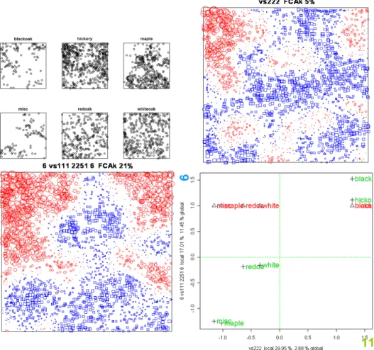
et al.2008). This is illustrated here using the dataset Lansing from spatstat. This dataset consist of an ecological study where categories of trees and their positions in the studied area are recorded. Analyzing the pattern of categories will help the ecologist to study tree associations in the development of the forest. A collocation of order 3 at distance 0.1 unit (square window of 1 unit × 1 unit) on the single point process marked with a categorical variable describing the tree species was used. The collocation functioncOO3d1S() is given in the file “v34i10-additions.R”. Other functions for other applications of the generic PTAk
method can be found atLeibovici (2004).
The function cOO3d1S() in the following code computes the collocation of order 3 for one marked point process, keeping the “locations of collocations” in one entry of the output ar-ray (instead of marginalizing for each category). Each cell nsi,j,k contains the number of
R> lansing.1 <- cOO3d1S(lansing, 0.1)
R> lansing.1.FCAk <- FCAk(lansing.1, nbPT = 3, nbPT2 = 3, minpct = 0.01,
+ modesnam = c("2251points", "6catTree", "6catTree"),
+ addedcomment = "S I I", chi2 = FALSE, E = NULL)
R> summary(lansing.1.FCAk)
++++ FCA3-modes++++ d = 0.1 unit
++ collocation Table lansing.1 2251 6 6 ++ S I I ---Total Percent Rebuilt---- 69.68052 %
++ Percent of lack of complete independence rebuilt ++ 42.70666 % selected pctoafc > 0.1 % total = 42.61869
-no- --Sing Val-- --ssX-- --Global Pct-- --FCA--vs111 1 1.000000 2.124032 47.08027 NA 2251 vs111 6 6 3 0.256438 1.074332 3.09603 5.85042 2251 vs111 6 6 4 0.062902 1.074332 0.18628 0.35201 6 vs111 2251 6 6 0.493220 1.429735 11.45302 21.64225 6 vs111 2251 6 7 0.250328 1.429735 2.95025 5.57495 vs222 11 0.238690 0.190229 2.68231 5.06863 6 vs222 2251 6 16 0.115381 0.092153 0.62677 1.18437 6 vs222 2251 6 17 0.103075 0.092153 0.50020 0.94521 vs333 21 0.132362 0.062104 0.82483 1.55865 6 vs333 2251 6 26 0.051125 0.024298 0.12306 0.23254 6 vs333 2251 6 27 0.048546 0.024298 0.11096 0.20967 ...
The FCAk() listing results obtained by the summary() function on a FCAk class object (in-heritance from “PTAk” class object) differs from the PTAk() listing multi-hierarchical tree of singular values by the extra column-FCA-percentage which is merely a percentage of variabil-ity without regard to vs111the trivial singular value 1. Associated with this trivial principal tensor we get the marginal FCA’s (or generally the marginal FCA(k−1)-modes).
R> plot(lansing.1.FCAk, mod = c(2, 3), nb1 = 6, nb2 = 11, lengthlabels = 5) R> lansing$marks <- lansing.1.FCAk[[1]]$v[6, ]
R> plot(lansing[lansing$marks< = 0], cols = "blue", + main = "6 vs111 2251 6 FCAk 21%")
R> par(new = TRUE)
R> plot(lansing[lansing$marks>0], cols = "red", main = "") R> lansing$marks <- lansing.1.FCAk[[1]]$v[11, ]
R> plot(lansing[lansing$marks< = 0], cols = "blue", main = "vs222 FCAk 5%") R> par(new = TRUE)
R> plot(lansing[lansing$marks>0], cols = "red", main = "")
Figure 7 displays some effects associated with spatial dependencies of the categories of trees as measured by the lack of independence for the collocation counts of order 3. The principal tensors 6 and 11 are indeed showing the same thing: collocations with Blackoak and Hickory
in the top left corner opposed to the collocations with Maple and Miscellaneous trees, and the reverse in the big blue squares areas. Nonetheless principal tensor 11 is a real third order
Figure 7: Main effects. Principal tensors 6 and 11 (see summary(lansing.1.FCAk)) from CAkOO analysis for collocation counts of order 3 of the Lansing data: blackoak, hickory, maple, misc, redoak and whiteoak trees.
discrepancy effect, and principal tensor 6 is like a second ordera posteriori as it is associated with a marginal effect (an FCA2-modes after marginal contraction, i.e., associated withvs111
which is all components values equal to 1 (thes= 0 of Equation24).
When analyzing cooccurrences of high orders on the same categorical variable, such as the
lansingdata, one gets lots of symmetries within the tensor to be analyzed byFCAk(). A fully symmetrical tensor can cause problems to obtain convergence for the actual algorithm within
SINGVA(). It is expected that the renewed interest in multiway tensor analysis, particularly for symmetric tensors (Ni and Wang 2007; Comon et al. 2008) will bring new algorithms for rank-one approximation (as in SINGVA() with the RPVSCC algorithm): see also Faber
et al. (2003) for a discussion on recent PARAFAC algorithms and de Silva and Lim (2008) for a general discussion on lower-rank approximation in general. Other multiway methods linked to higher order cooccurrences, spatially or non-spatially, are focusing on generalizing dissimilarities or similarities for multidimensional scaling. For example Bennani’s work from his thesis, published inHeiser and Bennani (1997), was looking at Euclidean approximation of 3-way dissimilarities using an approach generalizing the unfolding metric multidimensional scaling.
8. Penalized optimization
The optimization algorithm within PTA3() or PTAk(), can be seen as alternating uncon-strained least squares. Utilizing metrics could be seen as introducing linear constraints or linear smoothing, which was pushed a bit further by allowing any smoothing of the compo-nents within each iteration step. This very simple constraint makes a panelization algorithm which will be equivalent to using metrics or semi-metrics if the penalizing operators are linear in a separable Hilbert space, e.g., polynomial smoothing, spline smoothing (Leibovici and El Maˆache 1997;Leibovici 2008;Besseet al.2005). Nonetheless even in the previous case, the structure of the algorithm is more flexible, as for a particular mode, the smoothing parameter is a list of smoothers which can be different along the decomposition process. However, the increased flexibility of optimization may lead to an invalid or even non-convergent PTAk(), but nearly orthogonal decompositions may be intersting. Work to fully describe the proper-ties of such smoothing parameterization for the multiway methods in PTAk analysis is still underway by the current author.
Below is a comparison of two different PTA3 for a verbal study on 12 subjects in which brain activity is measured by fMRI during the verbal paradigm on/off showed by the square curves on Figure 8. The first analysis (top of Figure 8) is a standard PTA3-modes on the brain
× time × subject data, and the analysis at the bottom is using panelization for time and space: Wav2D() a 2-D wavelet smoothing for brain adapted from wavethresh and for time
a double kernel smoother Susan1D() provided in PTAk, which additionally to traditional kernel smoothing does preserve high peaks. The smoothing arguments inPTAk() or PTA3()
are then included: PTA3(..., smoothing = TRUE, smoo = list(Wav2D, Susan1D, NA),
...). Beforehand, the data was detrended, using Detren on the time mode and scaled for each subject using Multcent(). Only the first principal tensors are shown here, some more results especially combining metrics and penalization can be seen atLeibovici(2004).
Figure 8: Verbal study data brain × time × subject with: canonical PTA3-modes (top), penalisedPTA3-modeswith smooth constraints onbrain and time (bottom).