University of Pennsylvania
UPenn Biostatistics Working Papers
Year Paper
Variable Selection for Nonparametric
Varying-Coefficient Models for Analysis of
Repeated Measurements
Lifeng Wang
∗Hongzhe Li
†∗University of Pennsylvania, [email protected] †University of Pennsylvania, [email protected]
This working paper is hosted by The Berkeley Electronic Press (bepress) and may not be commer-cially reproduced without the permission of the copyright holder.
http://biostats.bepress.com/upennbiostat/art20 Copyright c2007 by the authors.
Variable Selection for Nonparametric
Varying-Coefficient Models for Analysis of
Repeated Measurements
Lifeng Wang and Hongzhe Li
Abstract
Nonparametric varying-coefficient models are commonly used for analysis of data measured repeatedly over time, including longitudinal and functional re-sponses data. While many procedures have been developed for estimating the varying-coefficients, the problem of variable selection for such models has not been addressed. In this article, we present a regularized estimation procedure for variable selection for such nonparametric varying-coefficient models using basis function approximations and a group smoothly clipped absolute deviation penalty (gSCAD). This gSCAD procedure simultaneously selects significant vari-ables with time-varying effects and estimates unknown smooth functions using basis function approximations. With appropriate selection of the tuning parame-ters, we have established the oracle property of the procedure and the consistency of the function estimation. The methods are illustrated with simulations and an application to analysis of microarray time-course gene expression data to in order to identify the transcription factors that are related to yeast cell cycle process.
Variable Selection for Nonparametric Varying-Coefficient Models
for Analysis of Repeated Measurements
Running Title: Variable Selection for Varying-Coefficient Models
BY LIFENG WANG AND HONGZHE LI
Department of Biostatistics and Epidemiology
University of Pennsylvania School of Medicine, Philadelphia, PA 19104, USA
SUMMARY:
Nonparametric varying-coefficient models are commonly used for analysis of data measured re-peatedly over time, including longitudinal and functional responses data. While many procedures have been developed for estimating the varying-coefficients, the problem of variable selection for such models has not been addressed. In this article, we present a regularized estimation proce-dure for variable selection for such nonparametric varying-coefficient models using basis function approximations and a group smoothly clipped absolute deviation penalty (gSCAD). This gSCAD procedure simultaneously selects significant variables with time-varying effects and estimates un-known smooth functions using basis function approximations. With appropriate selection of the tuning parameters, we have established the oracle property of the procedure and the consistency of the function estimation. The methods are illustrated with simulations and an application to analysis of microarray time-course gene expression data to in order to identify the transcription factors that are related to yeast cell cycle process.
Key words and phrases: Regularized estimation, Functional response, Longitudinal data, Time course gene expression data.
1. Introduction
Varying-coefficient models (Hastie and Tibshirani, 1993) are commonly used for studying the time-dependent effects of covariates on responses measured repeatedly. Such models can be used for longitudinal data where subjects are often measured repeatedly over a given period of time, so that the measurements within each subject are possibly correlated with each other
(Diggleet al., 1994; Rice, 2004). Another setting is the functional response models (Rice, 2004),
where the ith response is a smooth real function yi(t), i = 1,· · · , n, t ∈ T = [0, T], although
in practice only yi(tij), j = 1,· · · , Ji are observed. For both settings, the response Y(t) is a
random process and the predictor X(t) = (X(1)(t), . . . , X(p)(t))T is a p-dimensional vector of
random processes. In applications, observations for n randomly selected subjects are obtained
as (yi(tij),xi(tij)) for the ith subject at discrete time pointtij, i= 1, . . . , n and j = 1, . . . , Ji.
The linear varying-coefficient model can be written as
yi(tij) =xi(tij)Tβ(tij) +εi(tij), (1.1)
whereβ(t) = (β1(t), . . . , βp(t)) is a p-dimensional vector of smooth functions oft, andεi(t),i=
the number of covariates is small, depending on the designs of the studies, many methods have been developed for estimating the coefficients in Model (1.1), using parametric models (Diggle
et al., 1994) and nonparametric or semiparametric approaches (Zeger and Diggle, 1994; Lin and
Carroll, 2000; Rice and Wu, 2001; Huanget al., 2002). However, when the number of covariates
in Model (1.1) is large, one important problem is to select the important variables in such models.
The goal of this paper is to estimate β(t) nonparametrically and select relevant predictors
xk(t) with non-zero functional coefficient βk(t), based on observations {(yi(tij),xi(tij)), i =
1, . . . , n, j = 1, . . . , Ji}.
Regularized estimation has received much attention as a way of performing variable se-lection for parametric regression models (see Bickel and Li, 2006 for a review). Important regularization procedures for variable selection include LASSO (Tibshirani, 1996) and smoothly clipped absolute deviation (SCAD) (Fan and Li, 2001) and their recent extensions (Zou, 2006; Yuan and Lin, 2005; Zou and Hastie, 2005). However, these regularized estimation procedures were developed only for the parametric regression models where the model parameters belong to high-dimensional parametric space and cannot be applied directly to the nonparametric varying-coefficients models where the parameters are nonparametric smooth functions. Fan and Li (2004)
proposed to use the SCAD penalty for model selection in longitudinal data analysis when β(t)
are assumed to be time-independent. Wanget al. (2007) proposed a group SCAD (gSCAD)
pro-cedure for model selection for varying-coefficient models with time-independent covariates and demonstrated its application in analysis of microarray time course gene expression data. The goal of this paper is to further develop the gSCAD procedure for general nonparametric varying coefficients models with possible time-dependent covariate processes and to provide theoretical justification for the gSCAD procedure for variable selection and estimation. This procedure simultaneously selects significant variables and estimates unknown smooth coefficient functions. The rest of the paper is organized as follows. We first describe the general group SCAD regularized estimation procedure and the algorithm in Section 2. We then present theoretical properties of our estimators in Section 3, including the oracle property and the consistency of the estimates. Finally we present simulation results in Section 4 and application to analysis of microarray time-course gene expression data in Section 5. Proofs of the main results are presented in the Appendix.
2. Regularized Estimation Using gSCAD and Basis Function
Ex-pansion
In order to select the relevant covariates in Model (1.1), we propose a new method based on
basis expansion ofβ(t) and penalized estimation using a grouped version of the SCAD penalty.
In what follows, we assume βk(t) = P∞l=1γklBkl(t) ∈ Fk, where {Bkl(t)}∞l=1 are orthonormal
basis functions of function space Fk. Then βk(t) can be approximated by a truncated series
βk(t)≈PlL=1k γklBkl(t), and Model (1.1) becomes
yi(tij)≈ p X k=1 Lk X l=1 γklx(ik)(tij)Bkl(tij) +εi(tij), (2.1)
whereLk is the number of basis functions in approximating the function βk(t).
When the number of covariate pis small, Huang, Wu and Zhou (2002) proposed to estimate
Model (2.1) via a weighted least square regression. In this article, we propose using penalized least square regression for the sake of variable selection. Note that under the truncated series
approximations, each functionβk(t) in Model (1.1) is characterized by a set of parameters γk =
(γk1,· · · , γkLk)
T in Model (2.1). Instead of selecting nonzeroγ
kl in this model, we should select
nonzeroγk. This motivates the following group version of the SCAD regularized estimation; we
estimate γ= (γ1T, . . . ,γpT)T by by minimizing l(γ) =N−1 n X i=1 Ji X j=1 yi(tij)− p X k=1 Lk X l=1 γklx(ik)(tij)Bkl(tij) !2 + p X k=1 pλ(kγkk2), (2.2) whereN =Pn i=1Ji,γ= (γ1T, . . . ,γpT)T,γk= (γk1, . . . , γkLk) T,k= 1, . . . , p,kγ kk2 = (PLl=1k γkl2)1/2
is thel2-norm ofγk, andpλ(·) is the SCAD penalty function withλas a tuning parameter, which
is defined as pλ(|w|) = λ|w| if|w| ≤λ, , −(|w|2−2(2aaλ−|1)w|+λ2) ifλ <|w|< aλ, (a+1)λ2 2 if|w|> aλ. (2.3)
The penalty function (2.3) is a quadratic spline function with two knots at λ and aλ, where a
is another tuning parameter. Fan and Li (2001) showed that the Bayes risks are not sensitive
to the choice of aand suggested using a= 3.7, which was also used in this paper. Through ˆγ
which minimizes the objective function (2.2), an estimate of βk(t) can be obtained by ˆβk(t) =
PLk
To simply the expression of the objective function (2.2), we define B(t) = B11(t) . . . B1L1(t) 0 . . . 0 0 . . . 0 .. . ... ... 0 0 . . . 0 0 . . . 0 Bp1(t) . . . BpLp(t) , Ui(tij) = (xi(tij)TB(tij))T,Ui= (Ui(ti1), . . . ,Ui(tiJi)) T, andU = (U 1, . . . , Un). We also define y= (y1(t11), . . . , yn(tnJn))
T. The objective function (2.2) can then be written as
l(γ) =N−1 n X i=1 (yi−Uiγ)T(yi−Uiγ) + p X k=1 pλ(kγkk2). (2.4)
Remark 1. The requirement of the orthonormality of the basis{Bkl(t)}∞l=1is not essential. When
non-orthonormal basis{Bkl(t)}∞l=1 is used, the penalty
Pp
k=1pλ(kγkk2) in (2.2) and (2.4) should
be substituted accordingly by Pp
k=1pλ((γkTHkγ)1/2), where Hk = (hij)Lk×Lk is a matrix with
hij =
R
T Bki(t)Bkj(t)dt. The oracle property and convergence results in Section 3 still hold and
the proofs just need slight modification.
2.1. Algorithm
Because of non-differentiability of the penalized loss l(β), the commonly used gradient
method is not applicable. In this section, we develop an iterative algorithm based on local
quadratic approximation of the non-convex penaltypλ(kγkk2). Following Fan and Li (2001), in
a neighborhood of a given positive w0∈R+,
pλ(w)≈pλ(w0) + 1/2{pλ′(w0)/w0}(w2−w02).
In our algorithm, a similar quadratic approximation is used by substituting γ with kγkk2,
k= 1, . . . , p. Given an initial value of γk0 with kγk0k2 >0, pλ(kγk2) can be approximated by a
quadratic form
pλ(kγk0k2) + 1/2{p′λ(kγk0k2)/kγk0k2}(γkTγk−(γk0)Tγk0).
As a consequence, equation (2.4) becomes
l(γ) =N−1(y−U γ)T(y−U γ) +γTΣλ(γ0)γ, (2.5)
where Σλ(γ0) = diag{(p′λ(kγ10k2)/kγ10k2)IL1, . . . ,(p′λ(kγK0 k2)/kγK0 k2)ILp} with ILk an Lk
di-mensional identity matrix. This is a quadratic form, and can be solved by
We outline the algorithm as follows:
Step 1: Initialize γ(1).
Step 2: Setγ0=γ(m), and solve γ(m+1) by equation (2.6).
Step 3: Iterate Step 2 until convergence of γ.
In the initialization step, we obtain an initial estimation ofγusing a ridge regression, which
substitutes pλ(kγkk2) in equation (2.2) with a quadratic function kγkk22, and can be solved by
matrix operations. At any iteration of step 2, if some kγk(m)k2 is smaller than a cutoff value
ǫ1 > 0, we set ˆγk = 0 and treat x(k)(t) as irrelevant. If any matrix is singular when solving
equation (2.6), a small perturbation ǫ2 is added to the diagonal entry of the matrix. In our
algorithm bothǫ1 and ǫ2 are set to 10−3.
2.2. Selection of tuning parameters
To implement the proposed method, we need to choose the tuning parameters: Lk, k =
1, . . . , p and λ, where Lk controls the smoothness of ˆβ(t), while λ determines the sparsity. In
section 3, we show that the oracle property holds, when these tuning parameters grow or decay at
a proper rate withn. In practice, however, we need data-driven procedures to select the tuning
parameters. In this paper, we only consider the situation whenLk=Lfor allβk(t),k= 1, . . . , p.
To facilitate adaptive selection of L and λ, we propose using a closed form estimation of the
generalized cross-validation error (GCV) or the “leave-one-subject-out” cross-validation (SJCV) for two different situations: independent or correlated errors.
If the errors εi(tij) are independent for different tij, j = 1, . . . , Ji, an approximate GCV
is applicable. Note that in the last step of our algorithm, due to the convergence of γk, the
nonzero components are estimated as ˆγ = (UTU +N/2Σλ(ˆγ))−1UY, which can be considered
as the solution of a ridge regression as follows
ky−U γk22+N/2γTΣλ(ˆγ)γ. (2.7)
Consequently, the optimal (L, λ) can be approximately selected by minimizing the GCV error
for (2.7), which can be efficiently computed as
GCV(L, λ) = 1
N
ky−M(L, λ)yk22
(1−tr[M(L, λ)]/N)2,
If the correlation structure of ε(t) is unknown, the GCV is unsuitable. In such a situation,
we choose SJCV in the spirit of Rice and Silverman (1991), Hoover et al. (1998) and Huanget
al. (2002). Let ˆγ(−i) be the solution of (2.2) after deleting theith subject. The commonly used
cross-validation error is then defined as
CV(L, λ) = n X i=1 Ji X j=1 (yi(tij)−U(−i)(tij)ˆγ(−i))2.
CV(L, λ) is a good estimate of the true prediction error. However, its computation is very
intensive, since it requires solving equation (2.2)ntimes. To overcome this difficulty, we propose
using the following approximate cross-validation error
ACV(L, λ) = n X i=1 Ji X j=1 (yi(tij)−U(−i)(tij)ˆγ⋆(−i))2 = N X i=1 kyi−Uiγˆ⋆(−i)k22,
where ˆγ⋆(−i) is obtained by solving (2.7) instead of (2.2), deleting the ith subject. We have the
following “leave-one-subject-out” lemma (see Appendix A for the proof), which greatly facilitates the computation.
Lemma 1. Define y˜(i) = (y1T, . . . ,yTi−1,Uiγˆ⋆(−i),yiT+1, . . . ,ynT), and let γ˜(i) be the solution of
(2.7) with y substituted by y˜(i). Then, Uiγˆ⋆(−i) =Uiγ˜(i).
Note that ˆγ =Ay and ˜γ(i)=Ay˜(i). As a consequence of Lemma 1,
Uiγˆ⋆(−i)=UiAy˜(i)=Ui(
X
k6=i
Akyk+AiUiγˆ⋆(−i)) =Ui(ˆγ−Aiyi+AiUiγˆ⋆(−i)).
By some standard calculation, we have
yi−Uiγˆ⋆(−i) = (I −UiAi)−1(yi−Uiγˆ) = (I −Mii(L, λ))−1(yi−Uiγˆ). Therefore, ACV(L, λ) = N X i=1 k(I −Mii(L, λ))−1(yi−Uiγˆ)k22,
in which we only need to solve the inverse of theJi-dimensional matricesI−Mii. Then, we can
choose the optimal (L, λ) by minimizingACV(L, λ).
For the standard parametric linear regression models, Fan and Li (2001) established the or-acle property of the SCAD penalized estimates, which indicates that the SCAD penalty enables consistent variable selection and parameter estimation simultaneously, as if the subset of rele-vant variables is already known. We show that this oracle property also holds for our proposed gSCAD method for varying coefficients models. In addition, we also establish the consistency
and the convergence rate of our estimates of the smooth functions. Assume that onlyspredictors
are relevant in the Model (1.1). Without loss of generality, letβk(t),k= 1, . . . , sbe the non-zero
coefficients, andβk(t) = 0,k=s+ 1, . . . , p. We made the following technical assumptions:
Assumption 1: The subjects (yi(t),xi(t)), i= 1, . . . , n, are i.i.d., and the observation time
points tij are i.i.d. from an unknown density f(t) on [0, T], where f(t) are uniformly bounded
away from infinity and zero.
Assumption 2: The eigenvalues of the matrix E{X(t)XT(t)} are uniformly bound away
from infinity and zero for allt.
Assumption 3: There exists a positive constant M1 such that|xik(t)| ≤M1 for all t.
Assumption 4: There exists a positive constant M2 such thatEε2(t)≤M2 for all t.
DefineGk(Lk) ={g(t) =PLl=1k γklBkl(t)},ρn=Ppk=1infg∈Gkkβk−gkL∞,Ln= max1≤k≤pLk.
Hereρnis an approximation error of Gk(Lk) toβk(t),k= 1, . . . , p, which approaches zero as Lk
grows to infinity at a proper rate with sample size n. Furthermore, define
Ak(Lk) = sup g∈Gk(Lk),kgkL26=0
||g||L∞/kgkL2 , An= max
k Ak(Lk),
where kgkL∞ = supt∈[0,T]|g(t)|, and kgkL2 = (
R
[0,T]g(t)2dt)1/2. The following theorem, the
proof of which is given in the Appendix B, shows the oracle property, the consistency and the convergence rates of the estimates.
Theorem 1. Suppose the assumptions 1-4 listed above are satisfied, limn→∞ρn= 0 and
lim n→∞A 2 nLnmax{N−1 max 1≤i≤n(Ji), N −2X i Ji2}= 0. (3.1)
Then, with a choice of λn such thatλn→0 and λn/max{rn, ρn} → ∞, we have
(a.) βˆk = 0, k=s+ 1, . . . , p, with probability approaching 1.
(b.) kβˆk−βkkL2 =Op(max(rn, ρn)), k= 1, . . . , s, with rn= (N
−2L
Note that Theorem 1 gives the oracle property (1(a)) and the consistency (1(b)) for gen-eral basis choices for basis function approximations. The following corollary gives a specific convergence rates for a class of spline estimators (see Appendix C for the proof).
Corollary 1. Suppose that the assumptions in Theorem 1 hold, Ji =J, i= 1, . . . , n, and that
βk(t) have bounded second derivatives, k = 1, . . . , s, βk(t) = 0, k = s+ 1, . . . , p. Let λn → 0, n2/5λ
n→ ∞, and let{Bkl(t)}Ll=1k+4 be the cubic spline basis withLkequally spaced interior knots,
where Lk=O(n1/5), k= 1, . . . , p. Then,
(a.) βˆk = 0, k=s+ 1, . . . , p, with probability approaching 1.
(b.) kβˆk−βkkL2 =Op(n
−2/5), k= 1, . . . , s.
Note that the rate of convergence is the optimal rate for nonparametric regression with in-dependent, identically distributed data under the same smoothness assumptions (Stone, 1982).
4. Monte Carlo Simulation
We conducted simulation studies to assess the performance of the proposed procedure. In each simulation run, we generated a simple random sample of 200 subjects according to the
model used in Huanget al. (2002), which assumes
Y(tij) =β0(tij) +
23
X
k=1
βk(tij)xk(tij) +ε(tij), i= 1, . . . ,200, j = 1, . . . , Ji.
The first three variables xi(t), i= 1, . . . ,3, are the true relevant covariates, which are simulated
the same way as in Huang et al. (2002): x1(t) is sampled uniformly from [t/10,2 +t/10] at
any given time point t; x2(t), conditioning on x1(t), is gaussian with mean zero and variance
(1+x1(t))/(2+x1(t));x3(t), independent ofx1andx2, is a Bernoulli random variable with success
rate 0.6. In addition toxk,k= 1,2,3, 20 redundant variablesxk(t),k= 4, . . . ,23, are simulated
to demonstrate the performance of variable selection, where each xk(t), independent of each
other, is a random realization of a gaussian process with covariance structure cov(xk(t), xk(s)) =
4 exp(−|t −s|). The random error ε(t) is given by Z(t) + E(t), where Z(t) has the same
distribution asxk(t), k= 4, . . . ,23, andE(t) are independent measurement errors from N(0,4)
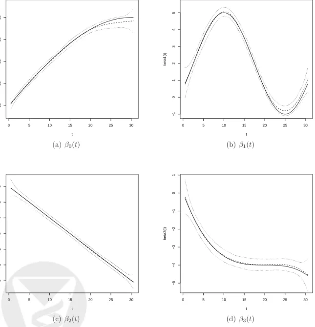
0 5 10 15 20 25 30 15 20 25 30 35 t beta0(t) (a) β0(t) 0 5 10 15 20 25 30 −1 0 1 2 3 4 5 t beta1(t) (b) β1(t) 0 5 10 15 20 25 30 0 1 2 3 4 5 6 t beta2(t) (c) β2(t) 0 5 10 15 20 25 30 −5 −4 −3 −2 −1 0 1 t beta3(t) (d) β3(t)
Figure 4.1: True (solid lines) and average of estimated (dashed lines) time-varying
term and the first three variables, are given by β0(t) = 15 + 20 sin( πt 60), β1(t) = 2−3 cos( π(t−25) 15 ), β2(t) = 6−0.2t, β3(t) =−4 + (20−t)3 2000 ,
(see solid lines of Figure 4.1) while the remaining coefficients, corresponding to the irrelevant
variables, are given by βk(t) = 0, k = 4, . . . ,23. The observation time points tij are
gener-ated following the same scheme as in Huang et al. (2002), where each subject has a set of
“scheduled” time points {1, . . . ,30}, and each scheduled time has a probability of 60% of being
skipped. Then, the actual observation time tij is obtained by adding a random perturbation
from U nif orm(−0.5,0.5) to the nonskipped scheduled time.
We repeated the simulations 100 times. Out of these 100 replications, the variables 1-3 were selected in each of the runs. Figure 4.1 shows the estimates of the time-varying coefficients of
βk(t), k = 0,1,2,3, indicating that the estimates fit the true function very well. As a
compari-son, among the 20 irrelevant variables, 10 were selected 1 time, 3 were selected 2 times, 5 were selected three times and 2 were selected 5 times. The simulations indicate that the proposed procedure indeed provides an effective method for selecting variables with time-varying coeffi-cients and for estimating the coefficient functions.
5. Application to Yeast Cell Cycle Gene Expression Data
We present results from our analysis of the yeast cell cycle microarray gene expression
data set of Spellman et al. (1998). They monitored genome-wide mRNA levels for 6178 yeast
ORFs simultaneously using several different methods of synchronization including anα
-factor-mediated G1 arrest, which covers approximately two cell-cycle periods with measurements at
7-min intervals for 119 mins with a total of 18 time points. Using a model-based approach, Luan
and Li (2003) identified 297 cell-cycle regulated genes based on the α-factor synchronization
experiments. In addition, we applied the mixture model approach (Chen et al., 2007) using
the ChIP data of Lee et al. (2002) to derive the binding probabilities xik for these 297
cell-cycle-regulated genes for a total of 96 transcriptional factors with at least one nonzero binding probability in the 297 genes. Our goal is to identify the transcriptional factors that might be related to the expression patterns of these 297 cell-cycle-regulated genes. Since different transcriptional factors may regulate the gene expression at different time points during the cell-cycle process, their effects on gene expression are expected to be time-dependent.
0 20 40 60 80 100 120 −0.2 −0.1 0.0 0.1 0.2 SWI6 Time beta(t) (a) Swi6 0 20 40 60 80 100 120 −0.8 −0.6 −0.4 −0.2 0.0 0.2 SWI4 Time beta(t) (b)Swi4 0 20 40 60 80 100 120 −0.4 −0.2 0.0 0.2 0.4 MBP1 Time beta(t) (c) M bp1 0 20 40 60 80 100 120 −0.4 −0.2 0.0 0.2 0.4 MCM1 Time beta(t) (d) M cm1 0 20 40 60 80 100 120 −0.3 −0.2 −0.1 0.0 0.1 0.2 0.3 FKH2 Time beta(t) (e) F kh2 0 20 40 60 80 100 120 −0.8 −0.6 −0.4 −0.2 0.0 0.2 0.4 0.6 NDD1 Time beta(t) (f) N dd1 0 20 40 60 80 100 120 −0.4 −0.2 0.0 0.2 SWI5 Time beta(t) (g) Swi5 0 20 40 60 80 100 120 −0.6 −0.4 −0.2 0.0 0.2 0.4 0.6 ACE2 Time beta(t) (h) Ace2 0 20 40 60 80 100 120 −0.4 −0.2 0.0 0.2 0.4 MCM1 Time beta(t) (i) M cm1
Figure 5.2: Estimated time-varying coefficients for selected transcription factors (TFs):
(a)-(c): TFs that regulate genes expressed at the G1 phase; (d)-(f ): TFs that regulate genes expressed at the G2 phase; (g)-(i) TFs that regulate genes expressed at the M phase.
We applied the gSCAD procedure using the GCV for selecting the tuning parameter in order to identify the TFs that affect the expression changes over time for these 297
cell-cycle-regulated genes in theα-factor synchronization experiment. The gSCAD procedure identified a
total of 71 TFs that are related to yeast cell-cycle processes, including 19 of the 21 known and experimentally verified cell-cycle related TFs, all showing time-dependent effects of these TFs on gene expression levels. In addition, the effects followed similar trends between the two cell-cycle periods. The other two TFs, CBF1 and GCN4 were not selected by the gSCAD procedure; it
was not clear why CBF1 and GCN4 were not selected by the gSCAD. The minimum p-values
over 18 time points from simple linear regressions are 0.06 and 0.14, respectively, also indicating that CBF1 and GCN4 were not related to expression variation over time. Overall, the model can explain 43% of the total variations of the gene expression levels.
Figure 5.2 shows that estimated time-dependent transcriptional effects of nine of the exper-imentally verified TFs. The top panel shows the transcriptional effects of three TFs, Swi4, Swi6
and MBP1, that regulate gene expression at the G1 phase (Simonet al., 2001). The estimated
transcriptional effects of these three TFs are quite similar with peak effects obtained at the time points corresponding to the G1 phase of the cell cycle process. The middle panel shows the transcriptional effects of three TFs, Mcm1, Fkh2 and Ndd1, that regulate gene expression at the
G2 phase (Simon et al., 2001). Again, the estimated transcriptional effects of these three TFs
are quite similar with peak effects obtained at the time points corresponding to the G2 phase of the cell cycle process. Finally, the bottom panel shows the transcriptional effects of three
TFs, Swi5, Ace2 and Mcm1, that regulate gene expression at the M phase (Simon et al., 2001),
indicating similar transcriptional effects of these three TFs with peak effects at the point points corresponding to the M phase of the cell cycle.
The 52 additional TFs that were selected by the gSCAD procedure almost all showed esti-mated periodic transcriptional effects. The identified TFs include many pairs of cooperative or synergistic pairs of TFs involved in the yeast cell cycle process reported in the literature
(Baner-jee and Zhang, 2003; Tsaiet al., 2005). Of these 52 TFs, 34 of them belong to the cooperative
pairs of the TFs identified by Banerjee and Zhang (2003).
Finally, to assess false identifications of the TFs that are related to a dynamic biological procedure, we randomly permuted the gene expression values across genes and time points and applied the gSCAD procedure again to the permuted data sets. We repeated this procedure 50
times. Among the 50 runs, 5 runs selected 4 TFs, 1 run selected 3 TFs, 16 runs selected 2 TFs and the rest of the 28 runs did not select any of the TFs, indicating that our procedure indeed selects the relevant TFs with few false positives.
6. Discussion
We have proposed a regularized estimation procedure variable selection for nonparametric varying-coefficient models. Such a procedure can simultaneously perform variable selection and estimation of the smooth functions and can be applied to both the longitudinal setting and the functional responses setting. The proposed gSCAD estimator have the oracle properties and is easy to solve using a local quadratic approximation algorithm. Simulation studies indicated that this procedure is very effective in selecting the relevant groups of variables and in estimating the regression coefficients. Results from application to the yeast cell cycle data set indicate that the procedure can be effective in selecting the transcriptional factors that potentially play important roles in regulation of gene expressions during the cell cycle process.
This paper focuses on linear varying-coefficient models; however, the proposed estimation procedure can be extended to more general regression models, such as the varying coefficients Cox regression model or the generalized linear models (Hastie and Tibshirani, 1993). Another possibility of extending the proposed work is to use smoothing splines for estimating the varying coefficients, with nodes chosen at the observed time points and a smoothing parameter to control the smoothness of the coefficients. We are currently pursuing these extensions.
Acknowledgments
This research was supported by NIH grant CA127334 and a grant from the Pennsylvania Department of Health. We thank Mr. Edmund Weisberg, MS at Penn CCEB for editorial as-sistance.
References
Banerjee N and Zhang MQ (2003): Identifying cooperativity among transcription factors
con-trolling the cell cycle in yeast. Nucleic Acids Research, 31: 7024-7031.
Chen G, Jensen S, and Stoeckert C (2007): Clustering of genes into regulons using integrated
modeling (CORIM). Genome Biology, 8, 1, R4.
Conlon EM, Liu XS, Lieb JD and Liu JS (2003): Integrating regulatory motif discovery and
genome-wide expression analysisProceedings of National Academy of Sciences, 100:
3339-3344;
Diggle PJ, Liang KY and Zeger SL (1994): Analysis of longitudinal data. Oxford: Oxford
University Press.
Efron B, Hastie T, Johnstone I and Tibshirani R (2004): Least angle regression Annals of
Statistics, 32, 407499.
Fan J and Li R (2001): Variable selection via nonconcave penalized likelihood and its oracle
properties. Journal of American Statistical Association, 96: 1348-1360.
Fan J and Li R (2004): New estimation and model selection procedures for semiparametric
modeling in longitudinal data analysis. Journal of American Statistical Association, 99:
710-723.
Hastie T and Tibshirani R (1993): Varying-coefficient models. Journal of Royal Statistical
Society, Ser B, 55: 757-796.
Hoover DR, Rice JA, Wu CO and Yang L (1998): Nonparametric smoothing estimates of
time-varying coefficient models with longitudinal data. Biometrika, 85: 809-822.
Huang JZ, Wu CO and Zhou L (2002): Varying-coefficient models and basis function
approxi-mation for the analysis of repeated measurements. Biometrika, 89: 111-128.
Lee TI, Rinaldi NJ, Robert F, Odom DT, Bar-Joseph Z, Gerber GK, Hannett NM, Harbison
CT, Thompson CM, Simon I, et al.: Transcriptional regulatory networks inS. cerevisiae.
Science, 298: 799-804.
Lin X and Carroll RJ (2000): Nonparametric function estimation for clustered data when the
predictor is measured without/with error. Journal of American Statistical Association,
Luan Y and Li H (2003). Clustering of time-course gene expression data using a mixed-effects
model with B-splines. Bioinformatics, 19, 474-482.
Rice RA (2004): Functional and longitudinal data analysis: perspectives on smoothing.
Sta-tistica Sinica, 14: 631-647.
Rice JA and Silverman BW (1991): Estimating the mean and covariance structure
nonpara-metrically when the data are curves. Journal of Royal Statistical Society B, 53: 233-243.
Rice JA and Wu CO (2001): Nonparametric mixed effects models for unequally sampled noisy
curves. Biometrics, 57: 253-259.
Schumaker LL (1981): Spline Functions: Basic Theory. Wiley, New York.
Simon I, Barnett J, Hannett N, Harbison CT, Rinaldi NJ, Volkert TL, Wyrick JJ, Zeitlinger J, Gifford DK, Jaakola TS and Young RA (2001): Serial regulation of transcriptional
regulators in the yeast cell cycle. Cell, 106: 697-708.
Spellman PT, Sherlock G, Zhang MQ, Iyer VR, Anders K, Eisen MB, Brown PO, Botstein D and Futcher B (1998): Comprehensive identification of cell cycle-regulated genes of the
yeast saccharomyces cerevisiae by microarray hybridization. Molecular Biology of Cell, 9,
3273-3297
Stone CJ (1982): Optimal global rates of convergence for nonparametric regression. Annals of
Statistics, 10: 1348-1360.
Tibshirani RJ (1996): Regression shrinkage and selection via the lasso. Journal of Royal
Statistical Society B, 58: 267-288.
Tsai HK, Lu SHH, and Li WH (2005): Statistical methods for identifying yeast cell cycle
transcription factors. Proceedings of National Academy of Sciences, 102(38): 13532
-13537.
Wang L, Chen G and Li H (2007): Group SCAD regression analysis for microarray time course
gene expression data. Bioinformatics, in press.
Yuan M and Lin Y (2006): Model selection and estimation in regression with grouped variables.
Zou H (2006): The Adaptive Lasso and its Oracle Properties. Journal of the American Statis-tical Association, 101(476), 1418-1429.
Zou H and Hastie T (2005): Regularization and variable selection via the elastic net. Journal
of Royal Statistical Society SER B-STAT MET, 67:301-320.
Zeger SL and Diggle PJ (1994): Semiparametric models for longitudinal data with application
to CD4 cell numbers in HIV seroconverters. Biometrics, 50: 689-699.
Appendix
Appendix A. Lemmas and proof
We first prove Lemma 1 that is related to leave-on-out cross-validation analysis. We then present and prove the other lemmas used in the proof of Theorem 1.
Proof of Lemma 1
: Use proof by contradiction. Suppose Uiγˆ⋆(−i) 6= Uiγ˜(i). Denote(2.7) aslridge(γ,y). Then, lridge(˜γ(i),y˜(i)) = n X k=1 ky˜k(i)−Ukγ˜k(i)k22+N/2(˜γ(i))TΣλ(ˆγ)˜γ(i) > X k6=i kyk−Ukγ˜k(i)k22+N/2(˜γ(i))TΣλ(ˆγ)˜γ(i) ≥ X k6=i kyk−Ukγˆk⋆(−i)k22+N/2(ˆγ⋆(−i))TΣλ(ˆγ)ˆγ⋆(−i) = lridge(ˆγ⋆(−i),y˜(i)).
This contradicts the fact that ˜γ(i) minimizeslridge(˜γ(i),y˜(i)), which proves the result. 2
Define ˜yi =E(yi|xi), ˜γ = (Pni=1UiTUi)−1(Pni=1UiTy˜i), and ˜β(t) =B(t)˜γ. Here ˜β(t) can
be regarded as the conditional mean of ˆβ(t).
To prove Theorem 1, we use the scheme as follows. First, using Lemma 2-3, we quantify the
convergence rate ofkβˆ−β˜kL2, which is established in Lemma 4. Then by Lemma 4, we prove
the consistency of variable selection in part (a) of Theorem 1. Finally, we improve the rate in Lemma 4 to obtain the rate in part (b) of Theorem 1.
Lemma 2. Suppose that (3.1) holds. There exists an interval [M3, M4], 0 < M3 < M4 ≤ ∞,
such that all the eigenvalues of N−1Pn
i=1UiTUi fall in [M3, M4]with probability approaching 1
as n→ ∞.
Lemma 2 and 3 are from Lemma A2 and A3 in Huang et al. (2002), respectively. The proofs are omitted.
Lemma 4. Suppose that (3.1) holds and thatλ≡λn,rnandρnapproach 0 asn→ ∞ satisfying
λn/max{rn, ρn} → ∞. Then, kβˆ−β˜kL2 =OP(rn+ (λnρn)1/2).
Proof of Lemma 4
: Because of the orthonormality of the basis,kβˆ−β˜k2L2 =
Pp
k=1kγˆk−
˜
γkk22 = (ˆγ−γ˜)T(ˆγ−γ˜). Let ˆγ−γ˜ = δu with δ a scaler and u a vector satisfying kuk2 = 1.
We first prove thatkγˆ−γ˜k2 =δ =Op(rn+λn).
Note that l(ˆγ)−l(˜γ) = N−1 n X i=1 (kyi−Ui(˜γ+δu)k22− kyi−Uiγ˜k22) + p X k=1 (pλ(kγ˜k+δukk2)−pλ(kγ˜kk2)) = (−2N−1 n X i=1 εiTUiu)δ+ (N−1uT n X i=1 UiTUiu)δ2 + p X k=1 (pλ(kγ˜k+δukk2)−pλ(kγ˜kk2)), (7.1) whereεi = (εi(ti1), . . . , εi(tiJi))
T. For the first term in (7.1), note that
Et(Bkl(t)2) = Z T 0 Bkl(t)2f(t)dt≤ sup t∈[0,T] f(t) Z T 0 Bkl(t)2dt = sup t∈[0,T] f(t), Then, E(εiUiu)2 = E( Ji X j=1 εi(tij)xTi (tij)B(tij)u)2≤E[ X j εi(tij)2 X j (xTi (tij)B(tij)u)2] ≤ JiM2E[ X j (xTi (tij)B(tij)u)2] ≤ JiM2 X j E[kxi(tij)k22kuk22tr{B(tij)BT(tij)}] ≤ JiM2pM32 X j Et( X k X l Bkl(tij)2) =O(Ji2Ln). As a result, N−1 n X i=1 εiTUiu=OP(E[N−1 n X i=1 εiTUiu]2)1/2 =OP(N−2Ln n X i=1 Ji2)1/2=OP(rn). (7.2)
For the second term in (7.1), by Lemma 2, (N−1uT n X i=1 UiTUiu)≥M3 (7.3)
with probability approaching 1.
For the third term in (7.1), note that |pλ(a)−pλ(b)| ≤λ|a−b|. Therefore,
p
X
k=1
(pλ(kγ˜k+δukk2)−pλ(kγ˜kk2)≥ −λkγˆ−γ˜k2 =−λδ. (7.4)
Combining (7.2), (7.3), (7.4) and the fact thatl(ˆγ)−l(˜γ)≤0, (7.1) becomes 0≥ −Op(rn)δ+
M3δ2−λδ with probability approaching 1, which implies kγˆ−γ˜k2 =δ =Op(rn+λn).
Now we proceed to improve the obtained rate and show that δ =OP(rn+ (λnρn)1/2). Note
that |kγˆkk2− kγ˜kk2|=op(1), and|kγ˜kk2− kβkkL2| ≤ kβ˜k−βkkL2 =Op(ρn), k= 1, . . . , p. We
have kγˆkk2 → kβkkL2 > aλn in probability,kγ˜kk2 → kβkkL2 > aλn in probability, k= 1, . . . , s,
and kγ˜kk2 = Op(ρn) < λn in probability, k = s+ 1, . . . , p, because λn → 0 and λn/ρn → ∞.
By the definition of pλ(·), it follows that P{pλn(kγ˜kk2) = pλn(kγˆkk2)} → 1, k = 1, . . . , s,
and P{pλn(kγ˜kk2) = λnkγ˜kk2} → 1, k = s+ 1, . . . , p. Combining with (7.2) and (7.3), with
probability approaching 1, we have,
l(ˆγ)−l(˜γ) ≥ N−1 n X i=1 (kyi−Ui(˜γ+δu)k22− kyi−Uiγ˜k22) + s X k=1 (pλ(kγ˜k+δukk2)−pλ(kγ˜kk2))− p X k=s+1 pλ(kγ˜kk2) ≥ −Op(rn)δ+M3δ2−Op(λnρn),
which implieskγˆ−γ˜k2 =δ=OP(rn+ (λnρn)1/2). This proves the desired result. 2
Appendix B. Proof of Theorem 1
To prove part (a) of Theorem 1, we use proof by contradiction. Suppose that there exists
a constant δ > 0 such that with probability at leastδ, there exist a large n and ak0 > s such
that ˆβk0(t)6= 0. Thenkγˆk0k2=kβˆk0(t)kL2 >0. Letγ∗ be a vector constructed by replacing ˆγk0
with 0 in ˆγ. Note that λn/max(rn, ρn) → ∞. Then, λn > kγˆk0k2 = Op(rn+ (λnρn)
probability approaching 1, and l(ˆγ)−l(γ∗) = N−1 n X i=1 (kyi−Uiγˆk22− kyi−Uiγ∗k22) +pλ(kγˆk0k2) = N−1 n X i=1 (−2yTi Ui(ˆγ−γ∗) + (ˆγ−γ∗)TUiTUi(ˆγ−γ∗)) +λkγˆk0k2 ≥ −Op(rn)kγˆk0k2+M3kγˆk0k 2 2+λnkγˆk0k2. (7.5)
Note that in (7.5), the third term dominates both the first term and the second term. This
contradicts the fact thatl(ˆγ)−l(γ∗)≤0, which proves part (a).
To prove part (b), first write γ = ((γ(1))T,(γ(2))T)T, where γ(1) = (γT
1, . . . ,γsT)T and
γ(2) = (γsT+1, . . . , γpT)T. Similarly, write β(t) = (β(1)T,β(2)T)T and Ui = (Ui(1),Ui(2)). Then
define the oracle version of ˜γ,
˜
γoracle = arg minγ=(γ(1)T
,0T)TN −1 n X i=1 ( ˜yi−Uiγ)T( ˜yi−Uiγ) = (P iU (1) i T Ui(1))−1(P iU (1) i T ˜ yi) 0 ,
which is obtained as if the information of the nonzero components were given. Note that the
true β(t) = (β(1)T,0T)T. Then by Lemma 3, kβ˜oracle −βkL2 = OP(ρn). To quantify kβˆ−
˜
βoraclekL2 =kγˆ−γ˜oraclek2, note that by part (a) of Theorem 1, with probability approaching 1,
ˆ
γ = ((ˆγ(1))T,0T)T. Let ˆγ−γ˜oracle =δu with u= ((u(1))T,0T)T and ku(1)k2 = 1. Then, with
probability approaching 1, l(ˆγ)−l(˜γoracle) = N−1 n X i=1 (kyi−Ui(˜γoracle+δu)k22− kyi−Uiγ˜oraclek22) = (−2N−1 n X i=1 εiTUi(1)u(1))δ+ (N−1(u(1))T n X i=1 (Ui(1))TUi(1)u(1))δ2 ≥ −Op(rn)δ+M3δ2,
which implies kγˆ −γ˜oraclek2 =δ = Op(rn). By triangle inequality, kβˆ−βkL2 = Op(ρn+rn),
and the result follows. 2
Appendix C. Proof of Corollary 1
By Theorem 6.27 in Schumaker (1981), infg∈Gkkβk−gkL∞ =O(L
−2
k ). Thusρn=O(Ppk=1L−k2),
and rn = (Ln/n)1/2 because Ji = J. Use Theorem 1 and solve ρn = rn. We obtain that