Identify Predictive SNP groups in Genome Wide Association Study: A Sparse Learning Approach

(1)

Procedia Computer Science 11 ( 2012 ) 107 – 114

Proceedings of the 3rd International Conference on Computational Systems-Biology and Bioinformatics (CSBio 2012)

Identify Predictive SNP groups in Genome Wide Association

Study: A Sparse Learning Approach

Zhuo Zhang

a,b,∗

, Yanwu Xu

b

, Jiang Liu

b

, Chee Keong Kwoh

a

a_{Nanyang Technological University, 50 Nanyang Avenue, Singapore 639798} b_{Institute for Infocomm Research, 1 Fusionopolis Way, Singapore 136238}

Abstract

Genome-Wide Association Study (GWAS) aims to identify genetic variants that are significantly associated with genetic traits. To analyze GWAS data that often contains 0.5 to 1 million Single Nucleotide Polymorphisms (SNPs) genotyped from thou-sands of individuals, stringent statistical significant thresholds are pre-defined for multiple testing adjustment, e.g., with p-value <10−8_{for single SNP detection and at least}_<₁₀−12_{for SNP-SNP interaction detection. Such stringent thresholds were used}

for eﬃciency computation but it hinders the discovery of many true genetic variants and more practical approaches are needed to conduct GWAS.

In this paper, we propose a machine learning approach to identify groups of predictive SNPs in GWAS analysis. Our method diﬀers from other methods by ﬁrst translates the genomics knowledge into SNP grouping as priors, then select a list of most predictive SNP groups using linear regression regularized by group sparse constraints, solved by Group-lasso (Least Absolute Shrinkage and Selection Operator). The selected SNPs groups compose a sparse feature space which yields a higher predictive power for continuous trait prediction.

We conduct experiment on SiMES (Singapore Malay Eye Study) data set, with 3280 Malay individuals genotyped on Illumina 610 quad arrays. We investigate one discrete trait (Glaucoma) and two glaucoma-related quantitative traits, optic Disc-Cup-Ratio (CDR) and Intraocular Pressure (IOP). The hypothesis is that, with more biological knowledge embedded, a learning mechanism yields higher predictive power. Our preliminary results support the above hypothesis. Further analysis reveals that our approach can identify groups of SNPs highly associated with a particular genetic trait, in spite of the small sample size and the incomplete biological knowledge.

c

2012 The Authors. Published by Elsevier B.V.

Selection and/or peer-review under responsibility of the Program Committee of CSBio 2012.

Keywords: single nucleotide polymorphism (SNP), genome wide association study (GWAS), regularized linear regression, least absolute shrinkage selector operation (lasso), group-lasso

1. Background

Genome Wide Association Study (GWAS) uses high-throughput genotyping technologies to assay hundreds of thousands of single nucleotide polymorphisms (SNPs) and associate them with the phenotype of interest; the identiﬁed SNPs are often used as genetic markers to identify the causes and access risks of disease. In a typical

∗_{Corresponding author}

Available online at www.sciencedirect.com

Open access under CC BY-NC-ND license.

(2)

GWAS data set, the number of SNPs (usually > 500k) far exceeds the number of sampled individuals (< 10k) by at least 50 fold. Computational methods have been investigated for SNP-trait association study due to its large number. Pioneer works [1, 2] focus on detecting statistically significant (e.g., with marginal effect) SNPs associated with a trait. Recently, efforts [3, 4, 5] have been expanded to investigate those SNPs with little effects on disease risk individually but influence the disease risk jointly, which is known as epistatic interaction in genetic analysis where the effects of one gene are believe to be modified by one or several other genes.

The single-locus and epistasis SNP detection based algorithms test individual SNPs or pair of SNPs without taking into consideration of the underline biological intertwining mechanism, whereas, the real gene-gene interac-tion participating in biological pathway are often composed by a group of SNPs with arbitrary numbers. However, to date, exhaustively detecting signiﬁcant SNP groups of arbitrary size is still computational infeasible.

In conventional GWAS, a significant statistical threshold is often set and only candidates passing the threshold are follow up. However, since SNPs are often correlated via linkage disequilibrium, the M most significant individual SNPs identified by simple linear regression may not constitute an optimal set for following up. It’s more important to find a small group ofN potent but interwinely correlated SNPs (some of them may not pass the stringent threshold by themselves) for following up study. In machine learning, such problem is classified as feature selection issue and regression methods are often used to tackle the challenges. However, a normal forward and backward stepwise regression cant address the sparse and correlated nature of genetic analysis. We explore penalized regression for its powerful engine and ability to perform continuous model selection when compared to the conventional regression approaches. It is also computationally suitable for large data analysis and adapts readily to the interactions of group members.

Penalized regression based on the Least Absolute Shrinkage Selector Operation (lasso) [6] were only recently been explored for GWAS analysis. Several lasso based approaches for GWAS analysis have been proposed. Some researchers [7, 8] proposed 2-step approaches for Genome-wide association analysis via shortlisting a group of marginal predictors using penalized likelihood maximization for further higher order interaction detection. Hoggart and others [9] proposed a method to simultaneously analyze all SNPs in genome-wide and re-sequencing association studies. D’Angelo [10] combined lasso and principal-components analysis for detection of gene-gene interactions in genome-wide association studies. These approaches are not global due to the 2-stage process and none of them have considered incorporating prior knowledge into the model building.

Prior knowledge can be combined into GWAS to improve the power of association study [11], it can also model dependencies and moderate the curse of dimensionality. In this study, we propose a holistic approach to identify groups of predictive SNPs in preliminary GWAS analysis. Our method translates prior knowledge of proteomics and biological pathways into SNP groups; we then apply linear regression regularized by group sparse constraint to select a small number of most predictive SNP groups, we use group-lasso as solver for the regularized linear regression.

The content of this paper is organized as follows. Section 2 describes methodologies for SNP grouping; group selection based on group sparsity constraint and regression model. Section 3 reports the preliminary experimental result. Section 4 concludes the study and points out our future work.

2. Methodology

2.1. Dataset

The presented work is based on data collected in a population based study, Singapore Malay Eye Study (SiMES) [12]. SiMES is a large-scale population based study to assess the causes and risk factors of blind-ness and visual impairment in Singapore Malay community, conducted over a 3 year period from 2004 to 2007 by Singapore Eye Research Institute and funded by the National Medical Research Council. A total of 3,280 individuals comprising Malay adults aged between 40 to 80 are genotyped on the Illumina 610 quad arrays. We only analyze the autosomal SNPs, and conducted a stringent quality control procedure and the ﬁnal set contains 2,542 individuals with 557,824 SNPs on 22 autosomal chromosomes. Clinical data collected for SiMES covers diagnosis information and various measurement of optic parameters. We choose three ocular traits because their signiﬁcance in ophthalmological study and their heritability presented in previous research [13, 14, 15, 16]. The discrete trait includes 121 glaucoma subjects and 2421 normal subjects. Two quantitative traits are optic Cup-to-Disc ratio (CDR), ranged from 0.08∼1.0 and Intraocular pressure (IOP), ranged from 6.0∼73 mmHg. The optic

(3)

disc is the anatomical location of the eye’s “blind spot”, the area where the optic nerve and blood vessels enter the retina. CDR is a measurement used in ophthalmology and optometry to assess the progression of glaucoma, which produces additional pathological cupping of the optic disc due to an increase in Intraocular Pressure (IOP). Single-SNP based GWAS has been reported previously for CDR [14, 15] and IOP [16].

2.2. Knowledge-based SNP grouping

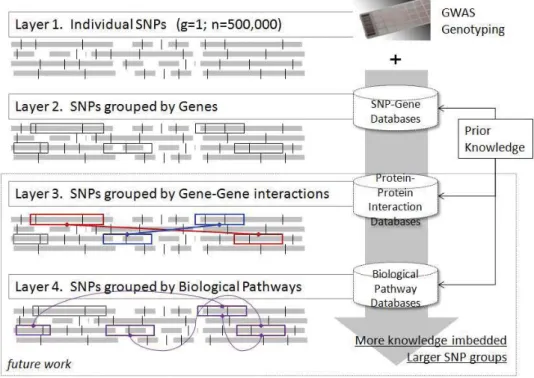
We group SNPs into cascading layers of functional units, as illustrated in figure 1. The first layer is individual SNPs; the second layer contains groups of SNPs located in the same genetic region. We use dbSNP [17] to annotate gene related SNPs. SNPs fall in extron, intron and flanking area within 10K distance from a gene are composed into one group. The approach makes it possible to detect well-annotated functional genes that are important to access the risk of interest genetic trait. The top-related SNPs in layer one are ranked by p-values obtained in basic association test as illustrated in section 3.1. Thefunctional SNP groups from layer two are selected by linear regression regularized by group sparse constraint which is illustrated in the section 2.4. In this preliminary study, we compare the predictive power of top-related individual SNPs selected from the first layer and SNP groups selected from the second layer. In future work, we will further introduce the third layer, where SNPs involved in protein-protein interaction genes are grouped together; and the fourth layer where SNPs that occur in the genes participating in one particular biological pathway form a group.

Fig. 1. A knowledge-based multi-layer SNP grouping mechanism

2.3. Linear SVR based continuous trait prediction

To predict IOP and CDR, which are continuous real values, from the very high dimensional SNP data, linear support vector regression(SVR) [18] is introduced for its eﬃciency; at the mean time, the accuracy can also be guaranteed since the feature dimension is signiﬁcantly higher than the number of training samples [19]. To improve from its initial implementation for feature selection and dimensional reduction, L2-regularized linear SVR [18] is introduced. For a sample with SNP featurefi, corresponding to a regression valueyi(i.e., CDR or

(4)

IOP value), a weighting vector ωis learned to predict the regression value usingωT_f

i+μ, by minimizing the following objective function:

min ω,μ l i=1 yi−ωTfi−μ2+Cω2 (1)

whereCis the regularization coeﬃcient which controls the generalization ability of trained model. 2.4. SNP group selection Based on Group Sparsity Constraint

SNPs may not aﬀect a particular trait individually, rather in a cooperative way which usually act in pairs or groups [20]. Thus, taking the relationship of SNPs in afunctional groupmay lead to higher prediction accuracy, and more importantly useful biological insights. By inspecting the contribution of the various layers, we can also infer the risk is caused by genes, protein complexes or regulatory pathways. At the same time, identifying and using only the eﬀective elements of the original features can bring about improvement in speed, and reduce computational cost.

For a sample with an original featurefi consisting ofgfeature groups (we treat each gene as a group), we denote its regression value (i.e., CDR or IOP value) asyi. We adopt the linear regression modelωT_f

i+μto obtain the estimated value, where ωis the weighting vector andμ is the bias, and minimize the following objective function: min ω,μ l i=1 yi−ωTfi−μ2+λ g j=1 ωj2 (2)

whereωj is the corresponding weight of the jth feature group,g is the number of groups, lis the number of training samples andλis used to control the sparsity ofω. In Eq. (2), the ﬁrst term represents the regression error and the second term is aL1,2-norm based regularizer to enforce the group sparsity. Considering the features are

intrinsically organized in groups, we use anL1,2-norm based regularizer to select features from only a sparse set

of groups. In the experiments, we use the group-lasso method provided in SLEP toolbox [21] to solve Eq. (2). Afterωis obtained with training, it can be used as a feature selection mask to generate the ﬁnal features,i.e., the jth _{group of features is selected when}_ω

j2 > 0. Usually, the selected feature has much lower dimension than the original feature, thus the subsequent prediction can be greatly speed up and the memory storage also be reduced signiﬁcantly.

Compare Eq. (1) with Eq. (2), one can observe that Eq. (1) is a special case of Eq. (2), in which all features are considered in an unique group; while in real cases, such high dimensional features are naturally grouped into many groups according to the functionality.

3. Experiment and Result

3.1. Single SNP based analysis

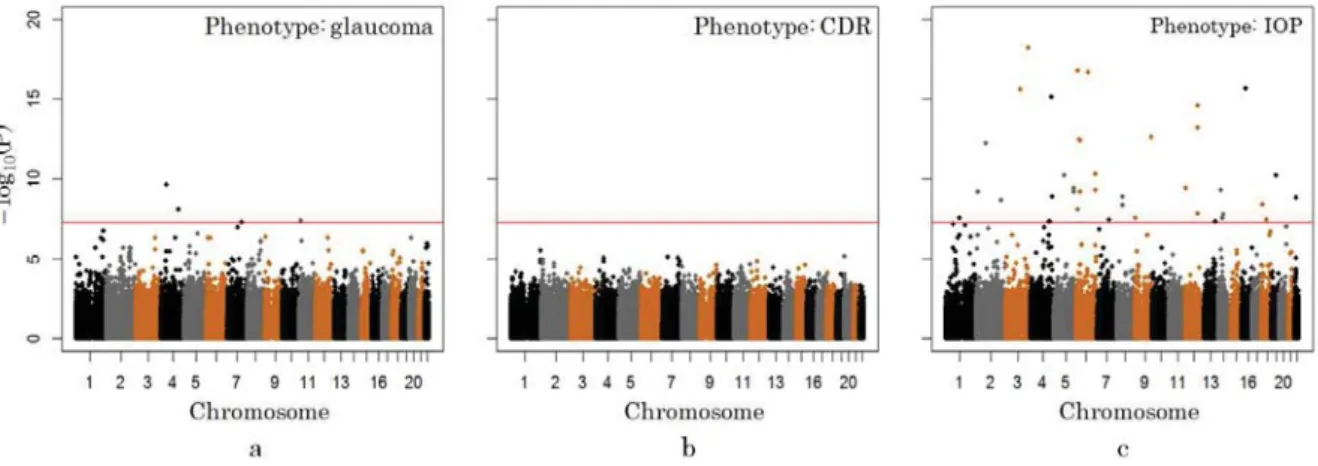
We first perform basic association analysis on the three traits for all individual SNPs, using software package PLINK [1]. The test basically calculates chi-squared statistic for each SNP against the respective traits. The resulted p-values are illustrated in the Manhattan plot as shown in Figure 2. Subplot a, b, c are Manhattan plots for glaucoma trait, CDR trait and IOP trait respectively. We observe that, with default genome wide significant setting (P <10−8_{), three SNPs are identified as significant SNPs for glaucoma. There is no significant SNP for}

CDR trait, and more than 20 signiﬁcant SNPs found for IOP. We rank the SNPs by their individual p-value and selected the top ranked SNPs as related features to construct prediction model. Top 400 SNPs for CDR and IOP trait are selected respectively.

3.2. Prediction based on selected SNPs

From the post QC GWAS data, we exclude samples with missing CDR or IOP values and focus on SNPs fall in genes or within 10K ﬂanking area of genes (as a preliminary study). It results in 2531 valid samples with 246,123 SNPs. In the 2531 samples, 1265 are randomly selected for training, which cover the whole range of regression values (CDR and IOP), the rest 1266 sample are used for testing.

(5)

Fig. 2. Manhattan plot for basic association analysis. a.Glaucoma; b.CDR; C.IOP

• Setting 1. The full SNPs feature set, contains about 246K SNPs.

• Setting 2. The high related feature set, 50-400 dimension, using top SNPs ﬁltered from association test as mentioned in last section.

• Setting 3. Sparse group feature set,< 500 dimension, SNP grouping is composed using prior knowledge and selected by group sparsity constraint. The SNPs grouping method is illustrated in Figure 1, in layer 2 the grouping unit is gene, layer 3 the group composes SNPs from a pair of interacting genes, and in layer 4 each group contains genes involved in a particular biological pathway. In this preliminary study, we focus on layer 2 grouping.

To compare the prediction power of diﬀerent SNP sets, we build the linear regression model for CDR predic-tion and IOP predicpredic-tion based on the three setting. The regression learning model of Setting 1 and 2 use Eq. (1) and Setting 3 uses Eq. (2). For fair comparison, optimal parameters are obtained with cross-validation on the training samples for each method. The parameter tuning are conducted as following:

• The regularizer coeﬃcientCfor linear SVR is set asC∈ {0.0001,0.001,0.01,0.1,1,10,100,1000,10000}

• The related feature set of Setting 2 is composed by top SNPs selected based on association test (as described in last section). 50, 100, 200 and 400 dimension top related features (SNPs) are tested

• For Setting 3, the group sparsity regularizer coeﬃcient is set asλ∈ {2000,4000,8000,16000} 3.3. Comparison of prediction power based on three feature sets

The regression results are evaluated by lowest average error obtained in each experiment, as listed in Table 1. In Setting 1, regression model is built on a feature space composed by all SNPs. We use the result of this setting as baseline to evaluate other Settings. Using all SNPs for learning introduces several issues. Firstly the sample size is too small compare to feature dimension and the learning can be easily resulted in overﬁtting during the training. We observe from Table 1 that training error is rather small (1.46% for CDR and 0.27% for IOP) but the testing error is much larger (12.62% for CDR and 3.94% for IOP). Moreover, the learning process consumes substantial memory and computational time. As most of the features are actually noise for the learning, in Setting 2, the feature space is composed by only the statistically most relevant SNPs, e.g., the SNPs with the lowest p-value. The regression result of Setting 2 leads to a poorer performance as compare to baseline, the reason can be the information loss in the whole genome context. In Setting 3, we use SNP groups to compose feature space, each group implies a functional unit in biological context which allows SNPs in the same group jointly aﬀect the trait. In both CDR/IOP cases the best testing performance are achieved in the Setting 3. The relative error reduction ratio (as compare to baseline) is 3.24% forCDR-Setting 3and 17.26% forIOP-Setting 3.

The prediction performance against number of selected SNPs (feature dimension) is illustrated in Figure 3. For CDR prediction, setting 2 with top 50 related SNPs yield good result, but more SNPs only introduces noises. For

(6)

Table 1. Optimal regression results for CDR and IOP Experiment Dimension (optimal) Training error (%) Testing error (%) Relative error reduction ratio (%) CDR

Setting 1 All SNPs 1.46 12.62 baseline

Setting 2 50 SNPs 12.20 12.76 -1.1

Setting 3 290 SNPs 12.14 12.21 3.24

IOP

Setting 1 All SNPs 0.27 3.94 baseline

Setting 2 400 SNPs 2.89 4.14 -5.1

Setting 3 381 SNPs 3.25 3.26 17.26

IOP prediction, the top related 50 SNPs do not yield optimal result and extra dimension gives better performance. The group SNPs (Setting 3) modeling outperformance Setting 2 with a reasonable dimension introduced.

L2-regularized linear SVR defined by Eq. (1) models a situation where features are consider as individual fac-tors. In Eq. (1), parameterCdetermines the trade-offbetween the training error and model complexity. Increasing Callows a more complex model, or more SNPs selected. On the other hand, L1,2-norm based regularized learning defined in Eq. (2) models the situation where the features work in groups jointly affecting the outcome. In Eq. (2) one can adjustλto control the group sparsity, a largerλ tends to reduce the number of selected groups and a smallerλwould allow more groups being selected. Accordingly, the x-dimension of figure 2 can be interpreted as the direction of decreasingλand increasingC, both yielding a larger number of selected SNPs.

0 100 200 300 400 500 11 12 13 14 15 16 17

number of related / group SNPs

av

erage error rate (%)

CDR Prediction

0 100 200 300 400 500

2468

1

0

number of related / group SNPs

av

erage error rate (%)

IOP Prediction

Prediction error related SNPs group SNPs all SNPs

Fig. 3. Prediction error rate on diﬀerent number of SNPs. Setting 1 - all SNPs; Setting 2 - related SNPs; Setting 3 - group SNPs To explore the underline biological function of the selected SNPs, we further analyze the 290 SNPs identiﬁed for CDR prediction in Setting 3. We match the SNPs back to genetic region, and look for a list of keywords in their gene page from NCBI gene database [22]. The relevant keyword list includes: Glaucoma, ocular, optic, macular, ciliary and retinal. From 290 SNPs, evidence shows that at least 21 genes are ocular-related, which provides a strong support for our approach.

4. Conclusion and future work

Sparse learning in high dimensional problems conducts feature selection naturally, which improves prediction accuracy and model stability. It also leads to a simpliﬁed model for faster prediction. More importantly, in this context, a small set of SNPs is desirable for further biological interpretation.

(7)

Table 2. Ocular related genes identiﬁed from selected SNPs

SNP Ids Gene Symbol Ocular-related description

rs17851391 CCNL2 Retinoblastoma

rs34315387 SCAMP3 Retinoic

rs10515929 SLC4A10 Glaucoma

rs17469794 LRP1B Optic

rs17701917 SPAG16 Cilia

rs11916441 KAT2B Retinoic acid

rs7433024 OTOL1 Maculae rs7614429 SUMF1 Retinal rs10071548 GPR98 Ocular ,Retinal rs7733024 GPR98 Ocular ,Retinal rs17847865 PPARD Retinal rs397576 BRD2 Retinoblastoma rs10486537 BBS9 Macular, Retinal rs11982601 DGKI Retina rs1078907 CHD7 Ocular rs16913039 TYR Ocular,Macular,Retina,Retinal rs1362629 ZNF423 Retinoic rs6500767 RBFOX1 Retinopathy rs11651398 DNAH17 Ciliary rs12449302 RNF135 Retinoic rs12449302 NF1 Optic

In a common GWAS, all SNPs are treated equally and assumed to work individually, which is often not true given our prior knowledge about candidate genes and biological pathways. The hypothesis is that, with more biological knowledge embedded, a learning mechanism yields higher predictive power. Our experiment results support the hypothesis. Our method diﬀers from the previously proposed approaches [7, 8, 9] that we incorporate prior knowledge into SNP grouping prior and then use sparse learning to identify the groups, the object function is optimized by improving the predictive power. The grouping priors can carry information on genes, protein-protein interactions or biological pathways. Our experiment demonstrates that the sparse feature space composed by gene-related SNP groups possesses higher predictive power in learning as compare to the whole-genome single-SNP or top-related SNP feature space. We believe that, with more complete prior knowledge and larger sample size, the approach can expect better result.

We will continue our work on SNPs grouped by Gene-Gene interaction as well as pathway. The predicted SNP groups can be used as a preliminary genome-wide scanning for further replication and validation.

Acknowledgements

This work was supported in part by the Agency for Science, Technology and Research, Singapore, under SERC grant 092-148-0073

References

[1] Purcell S, Neale B, Todd-Brown K, Thomas L, Ferreira MAR, Bender D, Maller J, Sklar P, de Bakker PIW, Daly MJ, Sham PC (2007) PLINK: a toolset for whole-genome association and population-based linkage analysis.American Journal of Human Genetics81. [2] Marchini J, and Howie B (2010) Genotype imputation for genome-wide association studies.Nature Reviews Genetics

[3] Wan X, Yang C, Yang Q, Yang H, Xue H, Fan X et al., (2010) BOOST: A fast approach to detecting gene-gene interactions in genome-wide case-control studies.Am J Hum Genet87: 325-340.

[4] Zhang X, Huang S, Zou F and Wang W, (2010) TEAM: e_ﬃcient two-locus epistasis tests in human genome-wide association study. Bioinformatics 26: i217-227.

[5] Wu J, Devlin B, Ringquist S et al. (2010). Screen and Clean: A tool for identifying interactions in genome-wide association studies. Genetic Epidemiology34(3), 275285.

(8)

[6] Tibshirani R. Regression shrinkage and selection (1996), via the lasso.J. Royal. Statist. Soc. B., 58, 267288.

[7] Wu TT and Chen YF and Hastie T and Sobel E and Lange K (2009), Genome-wide association analysis by lasso penalized logistic regression,Bioinformatics, 25(6),pp 714-21

[8] Wu Z, Aporntewan C, Ballard DH, Lee JY, Lee JS and Zhao H(2009), Two-stage joint selection method to identify candidate markers from genome-wide association studies,BMC Proc, 3(7), pp S29

[9] Hoggart CJ, Whittaker JC, De Iorio M and Balding DJ (2008), Simultaneous analysis of all SNPs in genome-wide and re-sequencing association studies,PLoS Genet, 4(7), pp e1000130

[10] D’Angelo GM, Rao D and Gu CC (2009), Combining least absolute shrinkage and selection operator (LASSO) and principal-components analysis for detection of gene-gene interactions in genome-wide association studies,BMC Proc, 3(7), pp S62

[11] Li C, Li MY, Lange EM and Watanabe RM. Prioritized Subset Analysis: Improving Power in Genome-wide Association StudiesHuman Heredity65(3): 129-141

[12] Foong AW, Saw SM, Loo JL, Shen S, Loon SC, Rosman M, Aung T, Tan DT, Tai ES, Wong TY. (2007) Rationale and methodology for a population-based study of eye diseases in Malay people: The Singapore Malay eye study (SiMES).Ophthalmic Epidemiol14(1):25-35. [13] Chang TC, Congdon NG, Wojciechowski R, Munoz B, Gilbert D, Chen P, Friedman DS, West SK. Determinants and heritability of

intraocular pressure and cup-to-disc ratio in a deﬁned older population.Ophthalmology2005 Jul;112(7):1186-91.

[14] Khor CC et. al. (2011), Genome-wide association studies in Asians conﬁrm the involvement of ATOH7 and TGFBR3, and further identify CARD10 as a novel locus inﬂuencing optic disc area.Hum Mol Genet.

[15] Wishal D. Ramdas (2010), A Genome-Wide Association Study of Optic Disc Parameters.PlosGenetics.

[16] van Koolwijk LM, Ramdas WD, et. al. (2012) Common Genetic Determinants of Intraocular Pressure and Primary Open-Angle Glau-coma.PLoS Genet.8(5):e1002611

[17] Sherry ST, Ward MH, Kholodov M, Baker J, Phan L, Smigielski EM, Sirotkin K (2001), dbSNP: the NCBI database of genetic variation. Nucleic Acids Res.29(1):308-11.

[18] Fan RE, Chang KW, Hsieh CJ, Wang XR and Lin CJ (2008), LIBLINEAR: A library for large linear classiﬁcation.Journal of Machine Learning Research9:1871-1874.

[19] Ho CH and Lin CJ (2012), Large-scale Linear Support Vector Regression.Technical report.

[20] Cantor RM, Lange K and Sinsheimer JS (2010), Prioritizing GWAS results: A review of statistical methods and recommendations for their application,Am J Hum Genet, 86(1) ,pp 6-22

[21] Liu J, Ji S and Ye J(2009), SLEP: Sparse Learning with Eﬃcient Projections. Techical report, Arizona State University. [22] http://www.ncbi.nlm.nih.gov/gene/