Visual Co-occurence Learning using Denoising Autoencoders

(1)

Visual Co-occurence Learning

using Denoising Autoencoders

Victor Deleau

A thesis

in

The Department

of

Computer Science and Software Engineering

Presented in Partial Fulfillment of the Requirements For the Degree of Master of Computer Science

Concordia University Montréal, Québec, Canada

August, 2020

c

(2)

(3)

Abstract

Visual Co-occurence Learning using Denoising Autoencoders

Victor Deleau

Modern recommendation systems are leveraging the recent advances in deep neu-ral networks to provide better recommendations. In addition to making accurate recom-mendations to users, we are interested in the recommendation of items that are comple-mentary to a set of other items. More specifically, given a user query containing items from different categories, we seek to recommend one or more items from our inventory based on latent representations of their visual appearance. For this purpose, a denoising autoencoder (DAE) is used. The capacity of DAEs to remove the noise from corrupted inputs by predicting their corresponding uncorrupted counterparts is investigated. Used with the right corruption process, we show that they can be used as regular prediction models. Furthermore, we measure experimentally two of their specificities. The first is their capacity to predict any potentially missing variable from their inputs. The second is their ability to predict multiple missing variables at the same time given a limited amount of information at their disposal. Finally, we experiment with the use of DAEs to recommend fashion items that are jointly fashionable with a user query. Latent repre-sentations of items contained in the user query are being fed into a DAE to predict the latent representation of the ideal item to recommend. This ideal item is then matched to a real item from our inventory that we end up recommending to the user.

(4)

Acknowledgements

I would like to thank my supervisor Jia Yuan Yu for allowing me to conduct my Mas-ter’s degree at Concordia. I learned greatly under his supervision, and am now a much better researcher than I used to be. I am also grateful to Volker Haarslev for giving me a chance to prove my worth before transferring to the Computer Science department, and more generally to the Concordia staff for their professionalism.

Thank you to Laurent Charlin for validating and encouraging the approach taken in this work. Many students in the lab and beyond helped me improve and finalize this thesis. Special thanks to Syed Eqbal, Denis Ergashbaev, and Tyler Manning.

I thank my uncles Loı̈c and Dominique for the model of exemplarity that they repre-sented to me. I also thank my aunts, my grandparents, and my mother Sylvie. They always provided me with love and help. My family in Quebec has also been particularly caring since my arrival, and I deeply thank them for that.

Finally, I could not call Montréal home without my friends Valentin Fleury, Mèét Patel, my cousin Sebastien, as well as the many other amazing people that I had a chance to meet. Special thanks to William Lim for having relentlessly watered my plants during the Covid19 pandemic.

(5)

List of Figures

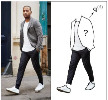
2.1 Representation of an incomplete queryQ¬i . . . 6

3.1 Boxcar and Gaussian functions with corresponding Fourier transform. . . 10

3.2 Hierarchy of recommendation systems . . . 12

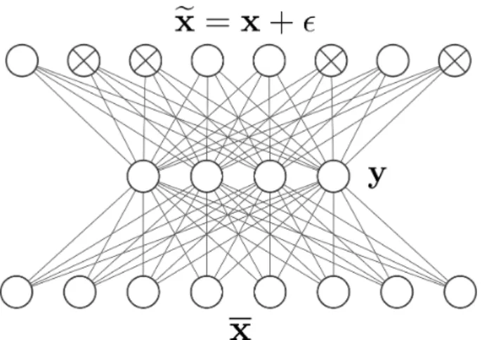
4.1 Representation of a vanilla 2-layer DAE . . . 23

4.2 Subset of prediction results on MNIST at epoch 190/200. . . 24

4.3 Manifold learning perspective: 2-manifold to 1-manifold mapping . . . . 25

4.4 Manifold learning comparison between VAEs and GANs. . . 26

4.5 Number of corruption masks perδmax with m= 9. . . 31

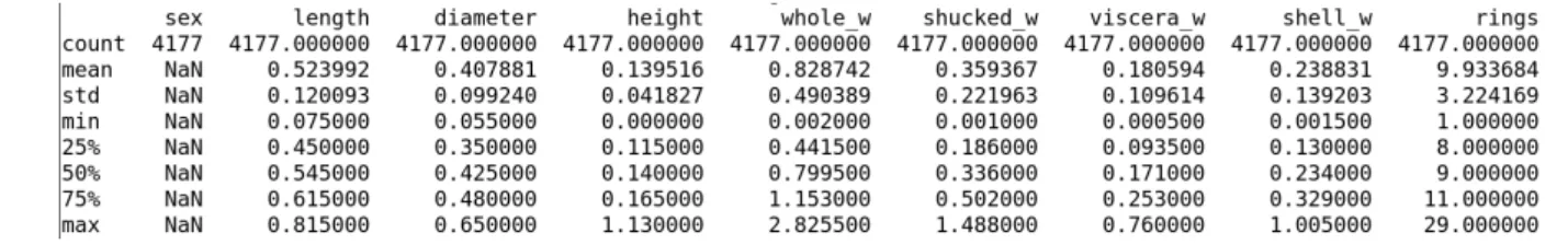
4.6 Statistics on each variable of the Abalone dataset . . . 31

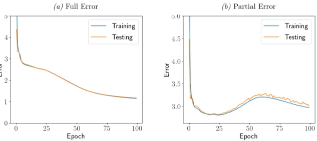
4.7 Full and Partial Error on the Abalone dataset,δmax = 1 . . . 34

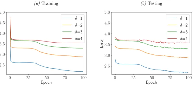
4.8 Partial Error per δ∈ {1,2,3,4} on the Abalone dataset,δmax = 4 . . . . 35

5.1 Dataset comparison. Partially taken from [19] . . . 44

5.2 Example of an outfit from the Polyvore Outfit dataset. . . 44

5.3 Full and Partial RMSE on Polyvore Outfit embeddings. . . 45

5.4 Partial RIRE score on the testing set of embeddings. Higher is better. . . 46

5.5 Example of an incomplete query with correponding ground truth item and predicted item . . . 48

(8)

1. Introduction

The massive economic growth of the 20th century brought people more freedom and wealth. We can now buy many goods for increasingly competitive prices, representing an increase in people’s buying power. But this has also led to a surge in the number of choices people have to make on a day-to-day basis. Customers are facing the problem of finding what they need in physical and online stores, and potential sales are sometimes not realized because of the customer’s inability to find what they need. From the retailer’s perspective, competition is getting fiercer with an increasingly polarized market, which calls for more value proposition and differentiation. Retailers are facing the challenge of satisfying increasingly demanding customers who want to find exactly what they have in mind and fast.

Those challenges are all but present in the fashion industry. With a compound annual revenue growth rate of 7.5% per year from 2014 to 2018 [13], the fashion industry is on the rise. Everybody buys clothing, and nearly all of us are concerned about the way we look and what society thinks about it. Being able to dress well, for the right situation, is perceived as a quality and makes one more attractive. Few of us master this skill, yet most would like to look better, which highlights the great innovative potential that remains untapped. The fashion industry is getting increasingly competitive, with a winner-take-all type of market that is pushing smwinner-take-all fashion retailers out of the race. According to the 2019 McKinsey technical report on the fashion industry [53], 97% of the profits in the fashion industry are now earned by only 20 companies, and most of them have doubled their profit during the last decade. So what are exactly the strategies put into practice by fashion retailers to adapt to this new reality?

One of the ways fashion retailers have been coping with those difficulties is by devel-oping recommendation systems. By collecting data on their customer’s behaviors, like historical purchases or implicit interactions, recommendation systems can propose a set of items that a customer would be more likely to appreciate and buy. First introduced in the 90’s, recommendation systems give an edge to the companies that are using them. They substantially increase the turnover of companies. For instance, 35% of what is bought on Amazon and 75% of what is watched on Netflix now come from recommenda-tions made by such algorithms [48]. Therefore, recommendation systems are now central to the success of not only fashion retailers but of all online retailers.

Originally based on traditional machine learning techniques, the field of recommen-dation systems is now benefiting from the latest development in artificial intelligence with the advent of deep neural networks. Autoencoders, a specific architecture of neural networks, highlight one of the major strengths of deep neural networks: their capacity to learn dense and abstract representations of high-dimensional and complex data. One of the domains where neural networks excel is in image-processing. Convolutional neural networks, either applied to image generation or classification, now bring an astonishing prediction accuracy. In the fashion industry, items benefit from rich annotations and peo-ple’s preferences for them are almost entirely based on their visual appearance. Discrete attributes are in their vast majority just a mere summary of the visual aspect of fashion items. By using convolutional deep neural networks, it is now possible to fully leverage

(9)

the visual appearance of fashion items to build better recommendation systems.

Beyond the simple recommendation of items to customers, it is also of interest to learn and recommend what goes well with what in situations where items are observed, bought, or worn together. In this work, we are interested in the problem of recommending complementary fashion items. As this notion of fashionability is not dependent on the user’s tastes but rather based on a more general and shared idea, this problem calls for an approach based on the content and appearance of items. Therefore, we leverage the visual aspect of fashion items to extract useful dense representations. We use a particular neural network architecture, a denoising autoencoder (DAE), and experimentally measure two of the characteristics that set it apart from other models, namely their robustness and versatility. We then experiment with the recommendation of complementary items on the Polyvore Outfit dataset and define our own ranking metric to assess the performance of our model.

In this work, we learn a notion of joint fashionability from a set of selected fashion outfits and assume that those fashion outfits are fashionable. This notion of fashionability is strongly related to the concept of style. But what exactly is a style?

1.1 What is a style?

It is well known that some very simple tasks for us humans can be particularly difficult or even impossible for machines to grasp, and conversely hard tasks for us humans can be easily solved by computers. In computer science, this is also known as the paradox of Moravec [1]. A good example of this is the concept of style. Let’s consider the style of paintings. At first sight, it is easy for us to distinguish between the style of two different pictorial artists but, until the recent advances in deep neural networks, computers had to combine various visual features extracted using classical techniques like SIFT [51] and SURF [5], as well as clustering algorithms to achieve modest classification results. Indeed, those methods were not able to extract the abstract content that images contain. Deep neural networks, especially applied to vision and language processing tasks, are now able to close this gap.

What we define by style is often highly dependent on the context, but we can still highlight some facts about this concept. First observe that one instance of a fashion style, an outfit, is made of several pieces of clothing that are assembled in a particular way. Each apparel of a given type also has a particular style, which helps us to compare it against other apparel of the same type. Therefore, styles discriminate.

Named styles, like chic or streetwear, are quick and easy to grasp references to some-thing that can be easily perceived and understood by others, but whose attributes are too complex or too large to be described one by one: it appeals to some kind of common understanding of the world. Giving names to some fashion styles facilitates communica-tion. In that sense, a style is also a compressed summary that is easier to communicate and manipulate. New named fashion styles are naturally created to classify and compare different outfits whenever the current set of commonly agreed upon named fashion styles doesn’t allow for a good enough characterization of what we want to express.

Neural networks, and more specifically autoencoders, are well suited for the task of understanding and representing styles. Due to their ability to extract dense lower-dimensional representations of their inputs while retaining and organizing most of the information that is characterizing them, it naturally draws similarity with the way we

(10)

process and communicate those concepts. This is why, in this work, we use deep neural networks to extract useful representations of the visual appearance of fashion items.

Now that we have defined the concept of a style, we argue about the underlying need that the fashion industry has for a unified way to recommend complementary fashion items. From there, we draw our motivations for this work.

1.2 Motivation for our work

In the last decade, researchers have been considering the problem of recommending com-plementary items through different angles. However, we believe there is still a significant area of improvement in this area of research.

Many of the methods that were previously proposed were considering pairs of items [29] [68] [41]. Some of them are also unidirectional [41], meaning that they consider an item with a given category as input and output an item from another target category. This implies that a new model must be trained for each pair of potential categories of items and each direction. Given that we might want to recommend items from a large number of different categories, this calls for a more flexible and integrated approach.

Some of the proposed methods are based on collaborative-filtering, a specific type of recommendation system that recommends items to users that similar users to them previously bought. An important issue with collaborative-filtering algorithms, and which they have by design, is their inability to recommend items when no information is known about the user. This is the so-called cold-start problem. Using the purchased history of users to learn the notion of joint fashionability that we are interested in is also problematic as unfortunately, not all users are style aware. Furthermore, co-purchased items do not necessarily imply the joint fashionability of those same items [42]. It is more sound to use a set of outfits that is selected by knowledgeable people and to learn the joint fashionability from the attributes and visual appearance of the items they contain. This would amount to a content-based approach, where customers are being recommended items whose attributes are similar to the one they previously interacted with. Note that there exist a lot of different fashion styles and that a given item could be part of two different outfits whose style is different. Therefore, such a recommendation system could still benefit from the user’s input regarding which of those styles the user prefers.

In a content-based recommendation setup, users are being recommended items whose attributes are similar to the one of items they previously bought. For this purpose, discrete attributes like color, category, and textual descriptions are often used. But is it the best way to characterize an item? While it depends on the actual context and type of items we are dealing with, in fashion, we believe that users’ behaviors are largely driven by the visual appearance of items. Furthermore, most of those discrete attributes are manually annotated and can be extracted in their vast majority from the visual appearance of items. To a lesser extent, this is also true for home furniture. Directly accessing the source of those discrete attributes could provide richer and more accurate representations of items, which would in turn lead to better prediction accuracy when fed to a prediction model.

Finally, in recent years we have observed new recommendation system models of increasing complexity. This added complexity does not always provide an increase in prediction accuracy [14]. In a real-life setting, several other aspects of a recommendation system might come into play. This includes ease of implementation and practicality of the

(11)

model that will be used in production: two things which might lead a decision-maker to not always select the best performing model that is known of. In this work, we recognize the importance of simple but effective approaches to solving problems.

To the best of our knowledge, if some of the previously proposed methods have been able to tackle few of the listed issues, none were able to solve all of them. Building on this knowledge, we now provide our goals for this work.

1.3 Goals

We seek a pure content-based approach that uses the visual appearance of items. As we focus on the recommendation of fashionable items, we can benefit from the availability of high-quality images that are always used to represent fashion items online. Some attributes cannot be extracted from the visual appearance of fashion items, such as fabric or country of origin. However, on average we believe that they do not participate greatly in the user’s choice and that consequently they can be ignored for this purpose.

We wish to design a versatile method to predict joint fashionability. By versatile, we mean that a single model should be able to recommend items from any of m different categories. Furthermore, we want to be able to complete an outfit by predicting multiple items from different categories at the same time. This amounts to making predictions using various amounts of information at our disposal, a capability that we denote as robustness. This is related to multi-task learning, a subfield of machine learning that is concerned with solving multiple tasks simultaneously. In this work, independently from the problem of recommending jointly fashionable items, we also seek to demonstrate the versatility and robustness of our solution experimentally on a classic machine learning dataset.

Finally, we want to demonstrate the capability of our model to recommend jointly fashionable items using a real-world dataset of fashion images. We seek a generic so-lution that can be applied to any situation where jointly fashionable items must be recommended. This also includes interior design for instance, and might or might not be based on visual data. The limitations of our proposed method will be truthfully listed such that it could be compared to other approaches.

1.4 Structure

Below is a short description of each chapter and its content.

In Chapter 2, we formally describe the problem that we are trying to solve, that is to jointly fashionable items, and introduce the notation that will be used throughout this work.

In Chapter 3, we review some of the most important research domains that are re-lated to our problem. Because our problem can be seen as a noise reduction problem, a background on noise reduction techniques will be first presented. We then introduce recommendations systems and present some of the most representative recommendation systems algorithms. Finally, we conduct a review of the literature on the specific task of recommending jointly fashionable items.

In Chapter 4, we formally define the model that will be used throughout this work, a DAE. We then provide an interesting perspective on what this kind of model is essentially doing by considering it through the scope of topology. Two characteristics of DAEs, that

(12)

we denote as robustness and versatility, are demonstrated. We outline our method and provide some arguments regarding its validity. The previously described method is then implemented, and experimental results are analyzed.

In Chapter 5, we try to solve the original problem of this work, which is to recommend jointly fashionable items. We first provide an argument as to why we believe DAEs could be used for this purpose. As in Chapter 4, we describe our method and then experiment on a fashion dataset. Experimental results are then analyzed. Finally, our solution is compared with previous works and its limitations are outlined.

We conclude by outlining the major points of this work. Several ways to improve the results we obtained are provided, as well as possible extensions to this work.

(13)

2. Problem statement

We are interested in the problem of recommending an item that is jointly fashionable to a set of other items based on their visual appearance. By saying that two or more items from different categories are jointly fashionable, we mean that they are likely to be observed together on fashionable outfits. In practice, each image would have to go through two steps that are the extraction of item regions from the image, or segmentation, and the extraction of visual features from items to obtain vectors of features. Vectors of visual features can be obtained through different means that we won’t detail in this section. For simplicity, the visual feature vector of an item will be directly referred to as an item. We first define how images, and the items they contain, are generated using a simple data generation model. Then, we introduce both an inventory of items to recommend and a query containing items for which the recommendation of a jointly fashionable item is requested. Finally, we propose a formal mathematical definition for the problem at hand. Consider an image that is i.i.d. sampled from some unknown probability distribution. Each image contains exactly m items, and each item in a given image is labeled with an element from the finite set C ={0,1, ..., m−1}, where the label corresponds to the category of the item. We assume that no two items in an image can be labeled with the same category. Each item is defined as a column vector a(i) _∈

Rk×1 of visual features,

where i ∈ C is the label of the item and k is the same for all items. Furthermore, item

a(i) is assumed to be i.i.d. sampled from a statistical distribution D(i)_{, of whom there is}

a total number of m for each label i∈C, such that D(i) ₌_proj

i(D). An image can then be represented as a matrix of items A ∈_Rk×m_{, such that} _A _{= [}_a(0)_,_a(1)_{, ...,}_a(m−1)_{], and}

a(i) ∼ D(i)_,_∀i_∈_C_.

(14)

In this problem, we assume that items are not combined chaotically inside images, and therefore that outfits are stylish. In situations where items are apparels or home furniture, this is a reasonable assumption. If they combined chaotically, then we couldn’t do better than recommending random items, and this problem would be trivial. This means that the column vectors ofA, which are random variables, are not independent of each other. It also means that, on top of considering the fashionability of standalone fashion items, the joint fashionability between fashion items should also be taken into account. Therefore, it must be possible to learn the joint distribution between the m different categories of items to provide recommendations. Note that here, item complementarity and joint fashionability are equivalent concepts.

In the problem at hand, a query must be given to the system in order to provide a recommendation. A query is an image provided by a user that is represented as a matrix of items Q = [q(0),q(1), ...,q(m−1)], where q(i) ∼ D(i)_,_∀i _∈ _C_{: this is referred}

to as the query. Additionally, we also define an incomplete query Q¬i as a query for which a recommendation of an item from a specific label i∈C is requested. Q¬i is such that its i ’th item is replaced with an arbitrary fixed value column vector Ø ∈ _Rk×1

which symbolizes the absence of the corresponding item from the query; namely Q¬i = [q(0), ...,q(i−1),Ø,q(i+1), ...,q(m−1)].

To recommend an item that would complement a given query Q¬i, we need an in-ventory of potential items to recommend. We define m different finite sets of items

I(i) ₌_{_p(i) 1 ,p (i) 2 , ...,p (i) ni} ∼ D (i)_,_∀i_∈_C_{, where}_n

i is the number of items in inventoryI(i). Note that, for a given instance of the problem, the content of the inventory is predeter-mined and fixed both in size and content across all possible queries, whereas a query Q

can be any possible composition of items observed inside a random image. Therefore, the quality of the recommendation is constrained by the size and content of the inventories. We can now formally introduce the objective of the problem at hand. Given an incomplete queryQ¬i, and for any label i∈C, we wish to recommend an item p(i) _from

our inventory I(i) as to maximize the fashionability of item p(i) with other items in Q¬i. This notion of fashionability is learned from a set of observations S ={Rj}nj=0S−1, where

each observation is an image represented as a matrix of items Rj = [r

(0) j ,r (1) j , ...,r (m−1) j ], such thatr(_ji)∼ D(i)_,_∀i_∈_C_{. Let} _p

.

(i) _{be the most complementary item to the incomplete}

query Q¬i in inventory I(i)_. _p

.

(i) _{can be estimated by maximizing the joint probability}

density between them different categories of items considered at p(i) _and _Q¬i

with S as a parameter. The objective can then be summarized as

arg max

p(i)_∈ _I(i)

f( p(i) , Q¬i ; S ) , (2.1)

Note that in practice f( · ; S ) is not the true joint probability density between items, but rather is a parameterized model that is set to estimate it as accurately as possible. Its parameters must be learned separately using a learning algorithm whose accuracy will depend, in part, on the number of observations nS. By unwrapping items in Q¬i,

f(· ; S ) can be rewritten as follow:

f( p(i) , Q¬i ; S ) =f(q(0) , ... , q(i−1) , p(i) , q(i+1) , ... , q(m−1) ; S ) (2.2) Furthermore, the higher the dimensionality of item vectorskand the number of categories

(15)

observations will be necessary to accurately estimate the true joint distribution of items. This is also known as the curse of dimensionality when solutions in low dimensions quickly become computationally prohibitive as the dimensionality increases.

In Equation 2.1, we try to find the best candidate amongst a limited set of items in the inventory, which can be seen as a classification of an incomplete query Q¬i into one of the potential items of the inventory. However, as we will later see and contrary to Equation 2.1, we will rather think about this problem as a regression task and not as a classification task. For this purpose, we use a specific version of the autoencoder architecture, the DAE. We first introduce the regular autoencoder framework before presenting its denoising variant. But first, we provide an overview of the subjects that are related to our work.

(16)

3. Related Work

3.1 Noise Reduction

A user query Q¬i whose item with label i is missing can be seen as a noisy signal. Removing the noise from Q¬i translates into finding an item that is most likely to be observed alongside items in Q¬i, i.e. the one that we should ideally be recommending. In that sense, our problem is related to noise reduction problems. In this section, we provide a short introduction to the problem of reducing noise as well as how it is done.

Noise reduction is the process of removing noise from a signal, where noise denotes an undesirable signal component. A noise is typically a random signal which can be characterized by its statistical properties. If a noise wasn’t random but deterministic, then the task of removing it would be trivial. Note however that noise can also be adversarial, in which case additional precautions must be taken. In practice, it is impossible to completely remove noise from a signal, and noise reduction will only result in a slight but useful increase in the Signal-to-Noise ratio (SNR). Noise reduction is critical in signal processing, and more specifically in telecommunications, speech recognition, or image processing.

There exists a wide variety of noises; the most common ones being white and pink noise. White noise has a constant power spectral density on a linear frequency scale and is naturally approximated by the thermal noise of charge carriers, like electrons in an electrical conductor. Pink noise has a constant power spectral density on a logarithmic frequency scale, which is also known as a Bode plot. Pink noise is often observed in biological systems. For instance, it has been observed as a response of biological systems stimulated with white noise [70]. Interestingly, the human perception of sound (and light) is known to be approximated by a logarithmic scale, which is why pink noise is commonly used as a calibration signal in audio engineering. This logarithmic perception is also known as Fechner’s law, which states that the perceived audio or visual stimulus is proportional to the logarithm of the stimulus intensity. Let p be the intensity of the stimulus that is perceived by an individual, Fechner’s law is such that

p=kln S

S0

, (3.1)

wherek is a constant, S is the physical intensity of the stimulus, and S0 is the minimum

stimulus intensity that can be perceived by the individual.

Noise reduction can be applied to any digital or analog signal. Consider a noisy signal

˜︁

x as the sum of a clean signal of interest and a noise signal, that is _˜︁x = x+ ϵ. A simple step to reduce noise in x_˜︁ is to model the statistical property of both x and ϵ. Then, according to those observed properties, the simplest approach to reducing noise is to filter some frequency bands more than others. For example, in two-dimensional representations of natural processes like photographs, the noise can often be considered to be a white Gaussian noise. White refers to the i.i.d. nature of the noise of each pixel, which allows one to consider each pixel’s noise as a random variable. This noise will

(17)

tend to increase high spatial frequencies in images, as most of the original information in images is located on the lower end of the spatial frequency spectrum. Therefore, filtering out high spatial frequencies would effectively reduce noise in the image.

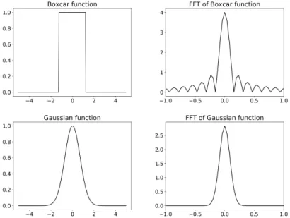
A basic approach to reducing high frequencies is to average the signal values over a given 2-dimensional window using a mean filter. Mathematically, this is achieved by convolving a boxcar function with the noisy signal _˜︁x. However, mean filtering will tend to increase some harmonic frequencies, which is undesirable. This is because the Fourier transform of the boxcar function is the Sinc function, and its absolute value has evenly-spaced high-frequency bumps as shown in Figure 3.1. Those high-frequency terms are also known as harmonic frequencies. In that regard, a better filter is the Gaussian filter whose Fourier transform is also a Gaussian function: consequently, the amount of applied filtering gently increases along with the frequency of the noisy signal _˜︁x. However, it is impossible to create an exact Gaussian filter either numerically and analogically, which is why they are often approximated.

Figure 3.1: Boxcar and Gaussian functions with corresponding Fourier transform.

It must be noted that filtering out high frequencies, depending on how flat the original signal’s spectrum is, will remove part of the original signal of interest as well. However, this is usually not noticeable if the cutoff frequency is high enough, as the human per-ception of visual signals is weakly sensitive to high frequencies. In practice, the flattest possible response in the signal band along with a steep roll-off in the stopband is often sought out. Better filters than mean or Gaussian filters are used for this purpose, like the Butterworth filter. Chebyshev filters of type I or II are also sometimes favored for their steeper roll-off in the stopband, with the drawback of being less flat in the passband.

We now provide more details on the low-pass Gaussian filter that is used to reduce the noise by filtering out high frequencies. Note that filters are also being reffered to as kernel. Considering the noisy signal as a function f : _R → _R, convolving f with a Gaussian kernel is known as a Weierstrass transform, which is a functional of the function

f that makes it smoother. The convolved Gaussian kernel can be defined as 1

√

4πte

−x2_/₄_t

(18)

where t controls the smoothness of the transformation. The one-dimensional generalised Weierstrass transform Wt[·] of function f is

Wt[f](x) = 1 √ 4πt ∫︂ y f(y)e−(x−4ty)2dy , (3.3)

which can also be expressed as a convolution

Wt[f](x) = 1 √ 4πt ∫︂ y f(x−y)e−y 2 4tdy . (3.4)

Interestingly, the generalised Weierstrass transform Wt[·] in 3-dimensional space can be used to accurately model the diffusion of heat in materials through time. Equation 3.2 is then referred to as the heat kernel, wheret becomes the time elapsed since heat diffusion began in the material. In fact, Joseph Fourier proved in 1822 that Expression 3.2 is the fundamental solution of the heat equation. Beyond physics, the generalised Weierstrass transform can also be used to make some functions easier to analyze. Indeed, it has been shown that if the Weierstrass transform of f exists between real numbers a and b, then it also exists everywhere in between. Furthermore, the Weierstrass transform generates analytical functions which are smooth by definition, hence infinitely differentiable.

The white Gaussian noise that we previously considered was static, in the sense that its statistical properties were stable over time. If the noise is dynamic, better filtering methods are available. The Kalman filter [31], by both estimating the expected signal using previous measurements and measuring the actual signal through time, can estimate the noise, or prediction error, by subtracting the two. Its performance can be tuned using the Kalman gain, which balances the importance given between current measurements and the estimation of the state of the noise and signal from previous measurements. The author Rudolf Kalman proved that the Kalman filter is the optimal linear filter if the noise is a white Gaussian noise whose parameters µY and σY are changing over time.

So far, the previously described noise reduction techniques only made use of the esti-mated statistical properties of the noise and signal. However, in most cases, we do have some prior knowledge about the signal of interest that can be leveraged. Given enough examples of noisy signals and their clean counterparts, we can train a machine-learning algorithm to denoise more effectively. For instance, convolutional DAEs have been suc-cessfully applied to noisy images [50]. Similarly, in this work, we use learning algorithms to denoise and hence predict what the original signal is given its noisy counterpart.

3.2 Recommendation systems

The problem of recommending complementary items is part of another important research domain, the one of recommendation systems. Numerous methods were designed since the advent of the internet in the 90’s. The major types of recommendation systems as well as their most representative algorithm are presented in this section. A literature review of previous work on the problem of recommending complementary items is then conducted. Recommendation systems are a specific type of information filtering system designed to predict which items in an inventory are most likely to be bought by users. They solve two problems. The first one is the discovery problem, that is the difficulty for customers to find the products they need online efficiently. For example, Amazon proposes more

(19)

than 12 million different products online, therefore helping their customers find what they need faster is a strong value proposition. The second problem that recommendation systems are solving is the one of increasing the retailer’s revenue. This is why some of the largest online retailers are willing to invest millions in research and development to improve their recommendation systems.

Recommendation Systems Content-based Collaborative-filtering Memory-based User-based Item-based Model-based Hybrid Figure 3.2:

Hierarchy of recommendation systems

Recommendation systems have been historically divided into two categories, namely collaborative-filtering (CF) and content-based filtering. Content-based recommendation systems recommend users items whose attributes are similar to those of items that they previously bought or interacted with. CF algorithms differentiate from content-based algorithms in that they do not need to understand or have access to the content of items they are recommending. They are rather based on the observed interactions between users and items. CF algorithms can be further divided into memory-based and model-based algorithms. Memory-based CF is concerned with predicting missing ratings as a function of other known ratings given by similar users (user-based) or received by similar items (item-based). Opposed to memory-based CF algorithms are model-based CF algorithms that are leveraging more advanced machine learning techniques to predict missing ratings. Finally, at the crossroads between content-based and CF recommendation systems, hybrid systems merge both approaches to get the best that each can provide [54] [4]. The relationship between those different methods is summarized in Figure 3.2 which proposes a hierarchy of recommendation systems. We now look more closely into these different types of recommendation systems and present some of their most representative algorithms.

3.2.1 Content-based

The first approaches to making recommendations were based on the item’s attributes and the preferences of users for those same attributes. Attributes can include information like color, category, texture, or even visual features like Scale Invariant Feature Transform (SIFT) [51]. Content-based recommendation systems have several limitations. The first one is that items must be annotated with attributes that can be processed by computers. Nowadays, there are almost no limitations on the kind of information a computer can

(20)

process, but this has not always been the case. Until recently computers weren’t able to fully understand the content of images for example. A second limitation of content-based algorithms is their limited ability to provide relevant recommendations. Let’s say for example that a given user has been buying a lot of DVDs online from the movie genre

Nouvelle Vague, a French art film movement of the late 50’s. Although this user only bought DVDs, it would be most natural for them to also be interested in literature on the

Nouvelle Vague genre, or even biographies of directors who initiated this art movement. Unfortunately, unless all items related to the Nouvelle Vague genre are annotated using a Nouvelle Vague tag, a content-based filtering algorithm won’t be able to pick up this relationship and will only recommend DVDs whose attributes are similar to the one the user has previously bought. A content-based approach can also be limited by the noisy nature of item attributes, which are often manually annotated and therefore error-prone. That being said, because content-based approaches are easy to implement and provide satisfactory performance, they are still being used extensively. We now present a simple content-based algorithm used for document recommendation and search, the Term Frequency-Inverse Document Frequency (TF-IDF) algorithm [39].

TF-IDF is one of the first and most popular content-based algorithms. It is used as a measure of relevance between a term and a document that is part of a corpus of doc-uments. Variations of TF-IDF were found in most search engines before being gradually replaced by more advanced Natural Language Processing (NLP) techniques. TF-IDF is made up of two measures, the term-frequency (TF) which measures the frequency of a term in a document, and the inverse document frequency (IDF), which measures the importance of a term in the corpus of documents by assigning it a weight that is inversely proportional to its frequency in the corpus of documents. It is often recommended to normalize the TF measure either by the maximum term frequency in the document or by the length of the document. Let ft,d ∈Nbe the raw count of term t in a documentd, and ld ∈N+ be the length of document d. The length normalized TF score of t in d is:

T F(t, d) = ft,d / ld (3.5)

LetD be a corpus of documents as a set, such that d∈D. The IDF score measures the specificity, or rarity, of a termt across all documents d∈D. It is traditionally defined as the logarithm of the total number of documents in the corpus D divided by the number of documents containing the termt:

IDF(t, D) = log |D|

|{d ∈D :t ∈d}| (3.6)

The final TF-IDF relevance score between a term t and a document d in a corpus D is

T F IDF(t, d, D) = T F(t, d)×IDF(t, D) . (3.7) Note that numerous variations of TF-IDF exist, most of them being based on how the TF and IDF scores are normalized, but all are fundamentally grounded on the same principles of term frequency and term specificity. TF-IDF is known to work very well as a heuristic, but the theory behind it is not well understood. Theoretical interpretations of it have been reviewed in [61]. We now look more closely into the other major type of recommendation systems, that is collaborative-filtering.

(21)

3.2.2 Collaborative-filtering

Let’s consider again our user who is interested in the Nouvelle Vague movie genre. By analyzing his purchase history, we can find similar users to him and realize that on top of buying DVDs on the Nouvelle Vague genre, those similar users also bought books on the Nouvelle Vague. A CF algorithm will be able to pick-up this relationship and recom-mend books on the Nouvelle Vague subject. In that regard, CF algorithms are generally considered to be superior to content-based algorithms [10]. However, a major drawback of CF algorithms is a decrease in their prediction accuracy as the sparsity of user-item observations increases. Indeed, usually, only a small subset of user-item interactions are observed. This eventually culminates with the impossibility to recommend anything if interactions between users and items are too sparse, an issue also known as the cold start problem. Hybrid recommendation systems, by integrating both CF and content-based filtering, were designed in part to solve this issue.

Memory-based CF

We now look more closely into CF. CF algorithms can be divided into two different sets of algorithms, namely memory-based and model-based algorithms. Memory-based algo-rithms are also known as neighbor-based and work by finding similar users, or neighbors, to the user we are interested in. It also has an item-based variant that considers similar items instead of similar users. Let’s consider as an example a simple memory-based CF algorithm based on the similarity between different users (user-based). The ratings given by neighbors to a specific item are combined using an aggregation function to predict the rating the user would give to this same item. Let Iu be the set of items that user u has rated, and ru,v be the rating given by user u to item v. We can define the mean rating

bu given by user u as:

bu = 1 |Iu| ∑︂ v∈Iu ru,v (3.8)

The predicted rating ̂ru,v given by useru to item v is then

̂ ru,v =bu+k N ∑︂ u′₌₀ w(u, u′)(ru′_,v−b_u′) , (3.9)

where w(u, u′) is a similarity metric between users u and u′, N is the total number of users, and k is a normalizing factor such that k∑︁N

u′₌₀w(u, u′) = 1. In practice, the

similarity functionw(u, u′) would often be a Pearson coefficient [60] or a cosine similarity [9]. Memory-based algorithms, just like content-based algorithms, are known to have scalability issues, as all observed ratings must be processed each time a prediction is requested. This makes the use of those algorithms challenging for online systems, where recommendations must be provided in real-time. Note that the prediction speed can be increased by approximating the nearest-neighbor search at the cost of lower prediction accuracy. This can be achieved either by keeping the top-N similar users to u as in [60], or by using a similarity threshold to discard users that are not similar enough.

(22)

Model-based CF

Opposed to memory-based CF algorithms are model-based CF algorithms, which try to model the underlying process that generates observed ratings. This often translates into learning what is known as latent factors. Due to its state of the art prediction accuracy and speed [10] amongst CF recommendation systems, matrix factorization (MF) methods are often favored. MF became widely known when Simon Funk discussed how good his model (dubbed Funk MF) was performing on the Netflix dataset in a blog post during the Netflix Prize competition in 2009. Inspired by the mathematical SVD decomposition, it consists of factorizing a sparse rating matrixR∈_Rm×n _{into two sub-matrices}_P_∈

Rm×k

and Q ∈ _Rk×n_{, also known as latent factors, such that} _r

u,v ∼ puqv, ∀(u, v) ∈ K where

K is the set of user-item pairs for which ratings are known. If the mathematical SVD is deterministic, matrix factorization is an optimization problem, and solutions are obtained using an iterative process. A benefit that MF has over mathematical SVD is that latent factors inPandQare forced to be non-negative, which is more practical. The biased MF variant proved to be very effective. It consists of separating the user, item, and global biases from the latent factors P and Q. This simple modification led to a significant increase in prediction accuracy. Biased MF was later improved by Koren et al. with SVD++[35] which added the implicit feedback that lies behind any user-item interaction, be it rated good or bad, as a sign of interest from users. timeSVD++[36] was later introduced to model temporal changes in users’ behaviors using trigonometric functions. Let’s consider as an example the biased SVD model proposed by Funk in 2009. The predicted rating ̂ru,v given by useru to itemv is given by

̂

ru,v =puqv +µ+bu+bv , (3.10)

where µ is the global mean rating, bu is the mean rating given by user u and bv is the mean rating received by item v. We can express the prediction error aseu,v =ru,v−r̂u,v. To avoid overfitting of the training data, a regularization term weighted by the hyper-parameter β ∈ _R+ _{is added to the loss as to penalize large value for the parameters,}

which are symptomatic of overfitting:

L= ∑︂

(u,v)∈K

e2_u,v+β(||p_u||2+||q_v||2+b2_u+b2_v) (3.11)

Latent factors P and Q are either learned using Alternative Least Square (ALS) or Stochastic Gradient Descent (SGD). ALS works by iteratively fixing p_u and solving for

q_v, and then conversely, for each pairs (u, v)∈ K. This gives a sequence of convex opti-mization problems that can be solved using the Ordinary Least Square (OLS) method, and for which a closed-form solution is known. Refer to Appendix 7.1 for more informa-tions on the closed-form solution of OLS. Gradient descent directly computes the gradient of the non-convex loss with respect to each parameter of the model before updating them. The stochastic variant of gradient descent uses the loss of each observed rating iteratively instead of using the combined loss over all observed ratings as in Equation 3.11. Both SGD and ALS are guaranteed to converge to a local minimum. A notable difference between the two is that with ALS the error is guaranteed to either decrease or stay the same, because of the convexity of the problem, whereas an SGD iteration can either increase or decrease the error. Let’s consider the SGD derivation as an example. The derivative of the loss function for a single observation (u, v) with respect to the user bias

(23)

parameter bu is

∂L ∂bu

=−2eu,v+ 2βbu (3.12)

Let η ∈ _R+ _{be the learning rate which controls how big of a step we take to update}

the parameters. The constant factor of 2 can be merged with the learning rate η for simplicity. With SGD, the parameters of the model are updated as follow:

bu ←bu+η(eu,v−βbu)

bv ←bv+η(eu,v−βbv)

p_u ←p_u+η(eu,vqv−βpu)

q_v ←q_v +η(eu,vpu−βqv)

(3.13)

SGD is often favored for the simplicity of its implementation, the speed at which pa-rameters are updated, and its capacity to sometimes cross ”bumps” in the loss function to escape a local minimum. ALS on the other hand provides longer but more accurate updates of the parameters. ALS also has the benefit of being easily parallelized, which allows the practitioner to train MF models on very large datasets. Parallelized versions of SGD, like DSGD [20] [40], were later proposed to address the issue of using SGD to train MF models on large datasets using a cluster of computers. Overall, a key benefit of model-based CF over memory-based CF and content-based systems is the ability of those CF models to make fast online predictions. This is at the cost of training a model be-forehand which can take a non-negligeable amount of time depending on the complexity of the model and the number of parameters.

Note that MF methods are linear, in that they try to model observed ratings by assuming a linear relationship between the unknown latent factors that we try to learn. However, linear models are fairly simple and might fail to accurately model the process that generates observed ratings. This led practitioners to experiment with non-linear models.

Neural approach to CF

Lately, many neural approaches to CF have been developed with the hope that the non-linearity of those models would help to design better recommendation systems. One of the first attempts at making recommendations using neural networks was proposed by Sedhain et al. with AutoRec [65], where a DAE was used to impute missing ratings in a sparse rating matrix. It has two variants, I-AutoRec and U-AutoRec, depending on how the rating matrix is being fed to the input layer of the DAE. Indeed, one can either slice the rating matrix in the column (item) direction or the row (user) direction. While an increase in prediction accuracy compared to their baselines was observed, they acknowledged that increasing the number of layers, which allows for more non-linearity of the model, only provided modest gains in prediction accuracy. This hints that CF latent factors can be effectively learned using simple models. In 2019, realizing that both user and item perspectives of the sparse rating matrix were complementary, Zhu et al. proposed a joint CF DAE architecture and reported an improvement in the top-k recommendation score [76]. Although our wortop-k is related to [65] and [76], we aren’t exactly in a CF setup and are rather concerned about a visual content-based approach to making recommendations.

(24)

algorithms hasn’t faded, with a large number of increasingly complex neural architec-tures being proposed for this purpose, each reporting a supposedly increase in prediction accuracy. This echoes the fact that, lately, applied machine learning researchers have been mostly focussing on absolute performance metrics [72], which doesn’t necessarily improve the quality of the perceived recommendation nor imply usability and practical-ity of the proposed solution in a real-life setting. A systematic review of neural-based CF algorithms as of 2019 was conducted in [14] and raised two problems. First, they found that research results were often difficult or even impossible to reproduce. This includes inaccessibility to the source code, unclear pre-processing steps, or an unknown initializa-tion method for the parameters. Second, baselines were sometimes badly tuned, which is in favor of proposed methods, and their choice is questionable. By implementing what could be reproduced with reasonable efforts, they found a second issue: most proposed solutions could be outperformed by well-known, decade-old properly tuned baselines. Generally speaking, it seems that traditional CF recommendation problems are solved to a point where no significant improvements in terms of absolute prediction accuracy could be gained. They concluded their work by calling for improved scientific practices in this area.

Recommendation systems are traditionally concerned about recommending a single item at a time to users. However, one might observe that items can also be used or ob-served together. Beyond the simple recommendation setup that we previously described, we now look at the specific problem of recommending items that are complementary to one another, something that is independent of user interests or past behaviors.

3.2.3 Recommending for joint fashionability

Recommending for joint fashionability is the task of recommending items that are jointly fashionable with one or more other items that are provided by a user.

An item-item CF approach can be seen as the first step toward this type of recommen-dation. Presented by Amazon in 2003 [42], this approach is popular under the headline ”Customers who bought X also bought Y”. For each item in the inventory, a list of other items with which it was co-purchased is kept. Instead of building an item-item matrix, which is memory intensive and doesn’t scale, they use an adjacency-list data structure to benefit from the highly sparse nature of item-item interactions. Given a currently considered item, the list of items with which it was co-purchased is filtered. In a CF setting, items can be represented as binary vectors of users, where elements set to 1 im-ply that users associated with the index of those elements interacted with the item. The similarity between two items can then be defined as the similarity between their two user vectors. The similarity between the user vector of an item and the user vector of every item with which it was co-purchased is computed. Co-purchased items are then sorted according to their similarity score, and the topN items are recommended, whereN is the number of items to recommend. Contrary to the memory-based CF approach described in Section 3.2.2, the lists of co-purchased items can be computed offline, which allows for faster online recommendations.

However, co-purchased items do not necessarily imply complementarity of those same items, and considering so is too strong of an assumption. A well-known legend in market-ing is the one of beer and diapers, which are supposedly often purchased together. Other than this potential relationship, these two items aren’t related in any other way. How-ever, gin, tonic, and lemons are clearly complementary, as they are consumed together

(25)

as part of the same recipe. For a notion of complementarity to be applicable is highly dependent on the context and type of items that are considered. Recently, the stock investing application Robinhood made a surprising usage of that kind of item-item CF recommendation system; the application recommended its users the stocks that similar users to them previously bought. The rationality behind such recommendation is highly debatable and could lead to errors of judgment from beginner investors. Beyond the absolute prediction accuracy of the recommendation, understanding the implication and relevancy of such recommendation is also important.

One of the first real attempts at recommending jointly fashionable items based on their visual appearance was proposed by Iwata et al. in 2012 [29]. They presented a Latent Dirichlet Allocation (LDA) model to match top apparel to bottom apparel and conversely. LDAs are part of the topic model family, a group of statistical generative models for discrete data that is frequently used in text-mining. They extracted top and bottom bounding boxes from photographs. Faces were located using a simple but accurate face detection algorithm [62]. Then, using common knowledge of human proportions, and knowing that their reference photographs were exclusively made of straight and camera facing persons, they deduced from the face’s position and size the position of the top and bottom apparel regions. After randomly checking extracted regions, they reported that 73% of images could be considered as being correctly extracted. A total of approximately 3,300 photographs were used. Color and Scale Invariant Feature Transform (SIFT) [51] features were extracted and concatenated into vectors. The topic model was then trained using them to learn the parameters of the Dirichlet distributions, as well as the latent top-ics, each latent topic being the equivalent of a fashion style. The top and bottom regions of each photograph were all encoded into low-dimensional vectors of topic proportions. Bottoms were matched to tops whose topic proportion was most similar, and conversely. One might observe that their region extraction process was suboptimal. First, the top region (and to some extent the bottom region as well) can contain one or more items, like a shirt, a scarf, or a jacket, and all of those items will be considered as a single top entity. Second, not all pixels inside the detected region are part of the actual items; in fact, most of them belong to the background whose visual features are irrelevant. Clearly, the performance they obtained could be improved by using more recent region extraction methods, like semantic segmentation neural network for instance.

In 2012, Liu et al. [44] created a recommendation system for the task of dressing for the right occasion and for recommending jointly fashionable items. They used an attribute-occasion Support Vector Machine (SVM) model for the task of dressing for the right occasion, and another attribute-attribute SVM model for the task of recommending jointly fashionable items. They manually annotated the top and bottom regions of 24,417 images with 10 occasion categories, and 7 apparel attributes, each being assigned to one or more values. Similarly to [29], top and bottom regions were extracted, but this time using a dedicated model that was proposed in [74]. Visual features including Histogram of Oriented Gradients (HOG) and Local Binary Patterns (LBP) were automatically ex-tracted from the top and bottom regions. Overall, positive results were obtained, and they noted the superiority of non-linear SVM models over linear SVM models. They also mentioned the importance of accurately extracting top and bottom regions as a pre-processing step, as misdetections would necessarily result in bad recommendations.

Extending the idea of matrix factorization used in collaborative filtering, in 2015 Hu et al. [26] proposed another approach to recommend jointly fashionable items. They

(26)

modeled user-item and item-item interactions by learning the latent factors of an M+1 order tensor, where M is the number of item categories. They simplified their problem by only considering 3 categories, namely top, bottom, and shoes. A gradient boosting method was used to map feature vectors from the feature space to a latent space. Their feature vectors included advanced versions of HOG and SIFT features. They gathered their training data from 150 users on Polyvore.com and obtained a training set of 180 positive outfits and 900 neutral outfits for each of them. The sparse tensor was factorized using functional gradient descent [52], a generalization of gradient descent that works in the generalized space of functions. A benefit that functional gradient descent has over traditional gradient descent is that a non-convex parametrized function can become convex in the function space. It is then possible for the model to avoid getting stuck inside of a local minimum. Although positive results were reported, the practicality of such a method remains to be demonstrated. Furthermore, the computational complexity induced by the functional gradient descent hasn’t been discussed. All-in-all, any imple-mentation would require a solid understanding of the complex mathematical theory that is involved.

In the fashion industry, the appearance of products is of utter importance. We believe manually annotated attributes to be in their vast majority just a compressed summary of the visual appearance of fashion apparel. It is well-known that low-level visual features like the one extracted by methods such as HOG or SIFT fail to extract the abstract content and meaning that images contain. Due to their capacity to learn complex pat-terns and their non-linearity, convolutional neural networks are able to fully leverage and understand the content of images. Therefore, a content-based approach based on latent features extracted from such models makes perfect sense and should theoretically provide better item representations, and therefore better recommendations.

One of the first attempts at recommending apparels using neural networks was pro-posed by Song et al. [68]. They propro-posed a content-based approach based on Bayesian Personalized Ranking (BPR). Instead of trying to optimize the error between a predicted rating and its ground-truth rating, BPR is rather concerned about the ranking of the most relevant items to recommend. Taking a sparse user-item matrix of interactions as input, and for a given user, BPR optimizes a ranking over all items for this specific user by using pairwise item preferences. BPR uses implicit interactions, like clicks on an item’s page or search queries, instead of explicit ones like ratings or scores. Pairs of item preference are made of an item with whom the user implicitly interacted with, denoted as the positive item, and of an item with which the user did not interact, denoted as the negative item. The underlying assumption is that users prefer items with which they implicitly interacted over others. Finally, using Bayes’ theorem, the posterior probability of a user to prefer positive items over negative items is maximized. This translates into maximizing the predicted score difference between the positive item and the negative item. It has been shown in the original paper of BPR [59] that BPR optimizes the Area Under ROC Curve (AUC) metric, a well-known machine learning metric, where the ROC curve is the plot of the true-positive rate as a function of the false-positive rate.

In 2018, Nakamura et al. [55] proposed a BiLSTM that generates a sequence of compatible items from different categories which are conditioned on the previous ones. LSTM stands for Long-Term Short-Term Memory and is a Recurrent Neural Network (RNN), a specific type of neural network that is generally used to process sequences of text. That being said, RNNs and by extension LSTMs can also be used to generate

(27)

sequences of any other kind of data, including latent representation of fashion apparels for instance. The bidirectional property of an LSTM refers to its added ability to process the data in both forward and backward directions. They used a pre-trained CNN model to extract latent representations of fashion items as a preprocessing step. Then, three different sub-networks were used: a Visual Semantic Embedding (VSE) network, used to join visual features and manually annotated attributes, a Style Embedding network (SE) whose task is to learn a style embedding from the whole outfit, and the BiLSTM model per se that is generating the sequence of items to recommend. Their work is based on a previous BiLSTM implementation for sequence of complementary items prediction [22]. Their contribution compared to [22] is to add the SE sub-module, which allows for fine-grained control of the generated outfit’s style. The downside of using an LSTM is that it requires multiple inferences for each item that must be generated, and that based on the previous sequence of items. In an online recommendation setting, a single inference is preferable.

In 2019, Lin et al. proposed a variational model that recommends new items based on a picture of what needs to be complemented and a textual description of the re-quested item [41]. More specifically, a visual representation of the predicted ideal item is generated. To avoid the generation of blurry images, an issue that is often observed when variational models are used along with Deconvolutional neural networks (DCNN), they separate the generative process in two stages. The first stage is a classic DCNN which generates a low-resolution image. The second stage is made of a super-resolution residual network (SRResnet) [38], which generates high-resolution images. Their model jointly learns a top encoder, a bottom encoder, and a top/bottom image generator. They advertized the superiority of this approach over the use of feature extractors made of pre-trained CNN models and reported a state of the art prediction accuracy over previous methods. Because their generator allows for the generation of either top or bottom items, we believe that this property could be extended to generate items from an arbitrary num-ber of item categories, hence bringing the versatility property that we are seeking in this work.

As in [68] and [22], we propose to directly extract visual features from fashion apparel using a pre-trained CNN. We now present the model that will be used throughout this work, the denoising autoencoder (DAE), and show how it could be used to recommend jointly fashionable items.

(28)

4. DAEs as flexible prediction

models

While applied machine learning researchers are often focused on absolute prediction ac-curacy [72], they often discard other traits such as practicality, flexibility, and resilience under degraded conditions. This contrasts with real-world implementations which are often made of less performant but more practical methods. We those goals in mind, we experiment with the use of Denoising Autoencoders (DAE). We first introduce this partic-ular architecture of neural networks, and provide an interesting perspective of their inner working. Two of their characteristics are then investigated, namely their robustness, and versatility. We describe our method for measuring these two qualities, before training a DAE on Abalone, a classical machine learning dataset. Finally, experimental results are analyzed, and the relationship between DAEs and multi-task learning is discussed.

4.1 Denoising Autoencoders

DAEs are a variant of the autoencoder framework defined in Appendix 7.2.3. Instead of taking a full vector as input to extract an embedding of lower dimensionality, like regular autoencoders, DAEs are rather provided with corrupted inputs and are given the task of reconstructing a complete and uncorrupted version of their inputs on their output layer as accurately as possible.

DAEs were initially used as predictive models, and not as feature extractors [67]. Along with convolutional layers, DAEs were later used extensively in image processing tasks to reduce the noise in images [50]. Convolutional layers can learn spatial patterns from the input data, contrary to fully connected layers which, as later demonstrated in Proof 5.2, are insensitive to the spatial ordering of their input values. Convolutional DAEs have also been used in super-resolution tasks [38], where the goal is to increase the definition of an image by inferring the value of missing pixels. It must be noted, however, that in image super-resolution tasks, there is no need to keep missing entries in the input layer, as their location is fixed and deterministic. If the position of missing entries is not known in advance, which is generally the case, then missing entries must be kept. In [50], Mao et al. showed the superiority of convolutional DAEs over traditional upscaling techniques like linear and cubic interpolation or even Gaussian smoothing, as well as for noise removal. Others have used DAEs to increase the Signal to Noise Ratio (SNR) of sonar images [33] or to restore and colorize old video footages [57]. Apart from being used as predictive models, a recent work by Vincent et al. in 2008 [71] demonstrated that randomly corrupting the input of DAEs, and eventually values in every subsequent layer, could also be used to help the model learn more robust representations, which ultimately led to better accuracy on classification tasks. In our case, we used DAEs as prediction models, and not to learn useful features. We now present a vanilla DAE and discuss its specificities.

If not otherwise stated, everything that applies to the autoencoder framework defined in Appendix 7.2.3 also applies to the DAE framework. Just like a regular autoencoder,

(29)

a DAE is made of an encoding function f : _Rk _→

Rk

′

and a decoding function g :

Rk

′

→ _Rk_{, respectively parametrized by the set of parameters} _ϕ _and _ψ_{. Contrary to} regular autoencoders, it is not necessary to apply regularization, as DAEs cannot learn the identity function: indeed, the model is forced to reconstruct on its output layer a piece of information that is different (because it is corrupted) than that of its input layer. Therefore, corrupting the input layer, and eventually, other subsequent layers, acts as a form of regularization, which prevents the model from overfitting and helps it generalize to unseen observations.

Inputs are corrupted using a corruption process. We define a corruption process as a function of both the input to be corrupted and of a corruption mask. Later in this work, we will define our own corruption process. Apart from containing some kind of randomness, there is no restriction on the nature of a corruption process. If it wasn’t partially random, then the DAE could learn a deterministic mapping of corrupted ob-servations to their corresponding uncorrupted versions: in other words, it would overfit the training set and fail to generalize to unseen observations. Let S ={xj}nS

−1

j=0 be a set

of nS observations, where each observation xj ∈Rk is i.i.d sampled from some unknown probability distribution q(X). Corrupted observations are obtained using a corruption process x_˜︁j ∼qD(˜︁xj|xj). The encoder and decoder functions are respectively defined as

y_j =f(_˜︁xj;ϕ) , ̂

xj =g(yj;ψ),

(4.1)

where ̂xj ∈ Rk is the predicted observation associated with the corrupted observation

˜︁

xj, and yj ∈ Rk

′

is known as the embedding or latent vector. A simple 2-layer DAE is shown in Figure 4.1. Similar to regular autoencoders, the sets of parameters ϕ and

ψ are updated through one or more epochs of Stochastic Gradient Descent (SGD) and backpropagation. In the case of a DAE, a training epoch can be generically defined as follow: ϕ, ψ←arg min ϕ,ψ 1 nS nS−1 ∑︂ j=0 L(xj, g(f(x˜︁j;ψ);ϕ)) , (4.2)

We say generically because in practice finding ϕ and ψ as to minimize equation 4.2 is not trivial when more than two layers are involved, and because equation 4.2 doesn’t tell us exactly how this is achieved. One can refer to the SGD and backpropagation techniques defined in Appendix 7.2.2 for more information on how to learn the model’s parametersϕandψ. Finally,Lis some arbitrary loss function whose choice is outside the scope of this section. In the DAE framework, it will generally be a discrepancy measure between uncorrupted observations xj and their corresponding predictions ̂xj such that

L : _Rk_×

Rk → R. Equation 4.2 can be expressed in more probabilistic terms. Let q0

be the empirical distribution associated with our set of training observations S. We are trying to learn the joint distribution

q0(X,X, Y˜︁ ) = q0(X)qD(X|X˜︁ )δ_f₍

˜︁

X;θ)(Y) (4.3)

where δu(v) is the Kronecker delta function which puts mass 0 when u ̸= v: this is defined as to show that Y is a deterministic function of X˜︁. The objective function 4.2

then becomes ϕ∗, ψ∗ = arg min ϕ,ψ E_q0₍_X,_X_˜︁₎ [︂ L(X, g(f(X˜︁;ψ);ϕ)) ]︂ (4.4)