Positive Tensor Network Approach for Simulating Open Quantum Many-Body Systems

Positive Tensor Network Approach for Simulating Open Quantum Many-Body Systems

1

Dahlem Center for Complex Quantum Systems, Freie Universität Berlin, 14195 Berlin, Germany 2

Institute for Complex Quantum Systems & Center for Integrated Quantum Science and Technologies (IQST), Universität Ulm, 89069 Ulm, Germany

3

Department of Physics, Colorado School of Mines, Golden, Colorado 80401, USA (Received 5 February 2015; revised manuscript received 18 February 2016; published 7 June 2016)

Open quantum many-body systems play an important role in quantum optics and condensed matter physics, and capture phenomena like transport, the interplay between Hamiltonian and incoherent dynamics, and topological order generated by dissipation. We introduce a versatile and practical method to numerically simulate one-dimensional open quantum many-body dynamics using tensor networks. It is based on representing mixed quantum states in a locally purified form, which guarantees that positivity is preserved at all times. Moreover, the approximation error is controlled with respect to the trace norm. Hence, this scheme overcomes various obstacles of the known numerical open-system evolution schemes. To exemplify the functioning of the approach, we study both stationary states and transient dissipative behavior, for various open quantum systems ranging from few to many bodies.

DOI:10.1103/PhysRevLett.116.237201

Open quantum systems are ubiquitous in physics. To some extent any quantum system is coupled to an envi-ronment, and in many instances this interaction signifi-cantly alters the system’s dynamics. Traditionally, such decoherence processes are seen as adversary to coherent state manipulation. However, suitably engineered dissipa-tion can also have beneficial effects and can be exploited for state preparation[1–8], even of states containing strong entanglement or featuring topological order. In condensed matter physics, many concepts such as transport are often studied within the closed systems paradigm, but it is becoming increasingly clear that some familiar concepts may have to be revisited in the open system setting [9], where the interplay between Hamiltonian interactions and dissipation leads to interesting physical effects.

Since few analytical methods are available for such systems, the design of novel numerical tools for the simulation of dissipative quantum many-body systems is of the utmost importance. In this work, we present a new algorithm that captures open many-body dynamics in one spatial dimension—for both transient and steady regimes— based on a locally purified tensor network Ansatz class. It comprises a new approach in that the positivity of the operators is maintained during the whole simulation. Importantly, the approximation errors can be controlled in a way that yields a trace-norm certificate. Hence, the algorithm provides not only a conceptually new approach to the problem, but also combines several desired features of existing schemes and overcomes previous limitations.

Tensor-network Ansatz classes have proven to be suc-cessful in capturing the physics of many-body states [10–15] by parametrizing a very small but physically relevant submanifold of quantum states with local corre-lations. The density-matrix renormalization method [16]

can indeed be viewed as a variational principle over matrix-product states [11,13,17–19]. Generalizing these ideas, a number of exciting methods have been proposed[20–26], some of which also allow us to study open quantum systems. In most cases matrix-product operators (MPOs) are at the heart of these methods. Indeed, several variants have already been developed [27–35], many of which exploit the well-known features of tensor networkAnsätze

to encode the mixed many-body quantum states in a compact matrix-product formulation, ultimately making the algorithm efficient and stable both for transient [27–29] and steady state physics[34].

However, in such a MPO description, the resulting truncated operators may not be positive; in fact, this property cannot even be tested locally, because it comprises a computationally intractable problem [36]. In Ref. [27] this is circumvented by dropping the positivity assumption during the time evolution, which requires that the approxi-mation errors remain sufficiently small. Alternatively, quantum jump schemes make use of a stochastic unraveling of the master equation [30,37,38] and then employ pure-state techniques, at the expense of having to sample over many realizations. The comparative performance of these two approaches has been recently investigated[39].

Remarkably, the subset of matrix-product operators that are cast in a locally purified tensor network (LPTN) form [27,40] shows promising features: such operators are positive by construction and exhibit all the helpful features typical of tensor networks. However, while the LPTN structure has been studied to represent boundary states in projected entangled pair tensor networks [26,41,42] a practical algorithm for one-dimensional open systems has yet to be formulated. Here, we show that such a positivity-preserving algorithm can actually be engineered for

Markovian dynamics: this scheme has the computational efficiency of tensor network methods, allows us to control all approximation errors in the operationally relevant trace norm, and preserves positivity by construction, thus ulti-mately merging the advantages of previous techniques while solving known issues.

Algorithm.—Our goal is to simulate the evolution of spin chains under local Markovian dynamics, i.e., one-dimensional lattice systems (at finite system size, with open boundary conditions) governed by the Lindblad master equation

dρ

dt ¼LðρÞ ¼−i½H;ρ þDðρÞ: ð1Þ Here, H¼PjHj is the Hamiltonian and the dissipative part of the Lindblad generator L takes the form

DðρÞ ¼P_αðLαρLα†−fL†αLα;ρg=2Þ, where the Lindblad operators Lα model the coupling of the system with the environment. We focus on the typical scenario, where the elementary Hamiltonian termsHjas well as the Lindblad operatorsLαare two local, meaning that they only couple spins on neighboring sites, and denote them byH½l;lþ1 _or L½l;lþ1_{, respectively.}

We describe the variational mixed state of the system as a tensor network representing the density matrixρ. But instead of expressingρdirectly as a MPO[27,43]we keep it at every stage of our algorithm in its locally purified form ρ¼XX†, where the purification operatorXis decomposed as a variational tensor network

½Xs1;…;sN r1;…;rN ¼ X m1;…;mN−1 A½1m1s1;r1A ½2s2;r2 m1;m2 A ½NsN;rN mN−1 ð2Þ

with1≤sl≤d, 1≤rl≤K, and 1≤ml≤D. Hence, we representρby a locally purified tensor network consisting of rank-4 tensors A½l _{with physical dimension d, bond} dimension D, and Kraus dimension K [see Fig. 1(a)].

Our algorithm is an extension of the time evolving block decimation (TEBD) scheme[44], acting on the level of the local tensor A½l _{that also allows for dissipative channels,} and never requires us to contract the two tensor network layers (X and X†) together. Similarly to TEBD, we split the propagator eτL for a small time step τ into several dissipative Trotter-Suzuki layers[45]of mutually commut-ing operators. Let us consider the evolution from time t to tþτ in row-wise vectorization jρ_tþτ⟫¼ je⟫τLρt¼ eτð−iH⊗1þi1⊗H¯þDÞ_jρ

t⟫, wherejM⟫denotes the vector given as the row-wise concatenation of a matrixM. As usual, for one spatial dimension (for possible generalizations to higher dimensions see the Supplemental Material [46]) we define the operators Ho and He by splitting the Hamiltonian H¼PN

l¼1H½l;lþ1 into two sums, one con-taining the even interactionsH½2l;2lþ1 and one containing the odd interactionsH½2l−1;2l_{. If the Lindblad operatorsLα} act only on site (the case of two-site Lindblad operators is treated later on), we can approximateeτL using a second order Trotter-Suzuki formula as (see the Supplemental Material[46])

eτL¼eτHo=2_eτHe=2_eτD_eτHe=2_eτHo=2þ_Oðτ3Þ_; ð₃Þ

partially shown in Fig.1(d), whereH_ν¼−iHν⊗1þi1⊗Hν¯ with ν¼o, e. The layers H_e and H_o implement the coherent part of the evolution and are identical to the usual TEBD layers. Expressingρ_tasρ_t¼XtX†t we find that by settingXt0¼e−iτHν=2Xtwe recover exactlyρt0 ¼eτHν=2ρt. Hence, for the coherent part of the dynamics, we can just adapt the usual TEBD algorithm for nearest neighbor Hamiltonians.

The dissipative layer requires a more careful treatment and we exploit the fact that since the operators L½l _act only on a single site, we findeτD¼⊗

le τD½l , with D½l¼ P j½L ½l j ⊗L¯ ½l j −ðL ½l† j L ½l j ⊗1þ1⊗L ½lT j L¯ ½l j Þ=2, where FIG. 1. Markov dynamics of a quantum spin chain on the level of local tensors. Panel (a) shows the relationship between a density matrixρin the MPO representation (top) and the locally purified tensor network (bottom) with tensorsAl, physical dimensiond, bond

dimensionD0, and Kraus dimensionK. (b) Action of a local channelTacting exclusively on lattice site 2 on the level of the MPO and on the level of the locally purified tensors. In the latter, the Kraus rank k2 of the quantum channel T is joined together with K. (c) Compression schemes for the bond and Kraus dimension of a local tensor via singular value decompositions (SVD). (d) Locally purified evolution of a time stepeτLfor a nearest neighbor Hamiltonian and on-site Lindblad operators. We only show three of the five Trotter-Suzuki layers from Eq.(3).

the sum runs over all Lindblad operators L½_jl acting on site l. Since eτD½l is completely positive, we can find a set of Kraus operators fBl;qg satisfying eτD½l ¼

P_k

q¼1Bl;q ⊗B¯l;q. The action of eτD

½l

on the level of the local tensors is now given by a contraction ofBl;qintoA

½l t , while joining the variational Kraus dimensionK with the Kraus rankk≤d2of the quantum channeleτD½l, as shown in Fig. 1(b). The application of each Trotter-Suzuki layer increases only the dimension of a single index of the local tensors A½l_{: the bond dimension D is increased by the} coherent layers, and the Kraus dimension K by the dissipative layers. This allows for immediate compression of the enlarged dimension similar to the standard density matrix renormalisation group setting. In all compression steps the Frobenius norm error introduced on the purifi-cation operators can be kept track of. This translates into a trace-norm error for the state itself. By taking also the error from the Trotter-Suzuki approximation into account, we obtain an explicit bound for the trace-norm error; see Theorem 1 in the Supplemental Material[46].

Numerical results.—In order to verify the applicability of our method we consider three prototypical benchmark situations. The first one comprises a few-body scenario, consisting of two qubits coupled via cavities with addi-tional excitation losses [52]. As a genuine many body example we study the steady state of an XXZ spin-1=2 chain with edge dissipation channels, which allows for comparison with analytical solutions derived in Ref. [9]. Finally, we show the validity of the two-site Lindblad-operator approach in the case of the Kitaev wire [7].

In the first model, two interacting optical cavities (C1and C2) are each coupled to a private qubit (S1 and S2). Ordering the sites asðS1−C1Þ−ðC2−S2Þgives a nearest neighbor model suited for our algorithm. The coherent part of the dynamics is captured by the Jaynes-Cummings Hamiltonian, which describes each spin-cavity interaction, plus a photon tunneling between cavities. In terms of the spin operatorsσ_l ¼ ðσx

l iσ y

lÞ=2and the creationc

†

l and annihilation operators cl of the cavity photons, the Hamiltonian is given by H¼Pl¼1;2ðαlðσþlclþσ−lc

†

lÞþ ωCnlþωSσzlÞ þαCCðc†1c2þc†2c1Þ. The dissipation mod-els a homogeneous probability of excitation losses and is given by single-site Lindblad operators: LS_l ¼pffiffiffiγσ−_l for the spins and LC_l ¼pffiffiffiγcl for the cavities. We start the evolution in a pure product state, where only the right cavity is nonempty and filled exactly with Nð0Þ ¼3 photons. The symmetries of the model imply an easy relation between the total excitation numberNðtÞand the coupling strengthγ: NðtÞ ¼Nð0Þe−γt, a behavior that is reproduced by our simulations with high precision (under 0.2% relative deviation). Figure2shows the occupation on each site as well asNðtÞ, which correctly reproduces the expected exponential decay. The inset shows the infidelity

Iðρ1;ρ2Þ ¼1−Tr½ðρ21=2_ρ1ρ21=2_Þ1=2 _{of the locally} puri-fied evolution ρ1 with respect to the exact evolution ρ2 carried out in Liouville space. As expected, close to the steady state the deviation of the locally purified dynamics from the exact evolution converges to a finite value (depending both on τ and the maximal bond D and Kraus dimensionK).

As a second benchmark, we consider the evolution of a spin-chain under the XXZ Hamiltonian H¼

P lðσxlσxlþ1þσ y lσ y lþ1þΔσzlσzlþ1Þ. Via a Jordan-Wigner transformation this system is mapped into a spinless fermion Hubbard model with a density-density nearest neighbor interaction. Therefore, with the addition of two reservoirs embodied by Markov channels at the edges, it models fermionic dc transport in a quantum wire. We introduce the Lindblad operators L← ¼pffiffiffiffiffi2γσþ₁ at the leftmost site (source) and L→¼ ffiffiffiffiffi2γ

p σ−

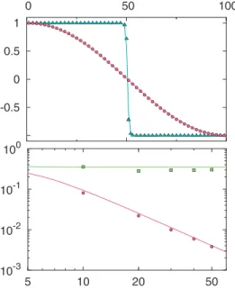
N at the rightmost site (drain). We identify the steady state for different parameter regimes ðΔ;γÞ. For comparison with analytic results from Ref. [9], we consider the local z axis magnetization σz_l and the spin-current operator Il¼ iðσþ_lσ−_lþ1−σ−_lσþ_lþ1Þ. The steady state regime is achieved by evolving the system until these observables become stationary. Figure 3 shows the local magnetization of a chain ofN ¼100spins in the top panel, while the current as a function of the chain length is plotted on the bottom frame. A remarkable quantitative match to Ref.[9]emerges even for smallDandK (∼60).

Finally, we consider a setting with two-local instead of on-site Lindblad operators (see the Supplemental Material [46] for details). We employ a two-layer Trotter-Suzuki

0.1 1 0 20 40 10-7 10-3 0 30 60

FIG. 2. Main: excitation populations of the four sites (see the main text) in the coupled spin-cavity model (yellow, cavity; violet, spin; dashed, right; straight, left), here for γ¼0.05, α1¼α2¼0.48, α_CC¼−1.0,ω_C¼ω_S¼1.0, as well as their sumN (green line). The latter is nicely fitted by an exponential, with decay rateγfit¼0.049978×10−5. Inset: comparison of the locally purified evolution, here for bond dimensionD¼40

and Kraus dimensionK¼40, with the exact Liouville evolution: infidelityI(blue line) and relative Hilbert-Schmidt distance (red line). Infidelities are estimated to be numerically reliable above

approximation with odd L_o¼H_oþD_o and even L_e¼

HeþDeterms. After computing the Kraus decomposition for the corresponding nearest-neighbor channelseτL2l;2lþ1¼

P_k

qB ½2l;2lþ1

q ⊗B¯½2ql;2lþ1one can choose how to implement the action of B½2ql;2lþ1 onto A½2l andA½2lþ1. In particular, there are different possibilities for distributing the Kraus rankk of the channel between the Kraus dimensionsK2l andK2lþ1 of the two sites.

Moreover, when such a dimension kis distributed non-trivially (k1>1to the left site, andk2>1to the right site, wherek1k2¼k) there is an additional freedom, represented by a unitary transformationUin thek-dimensional auxiliary space, that influences the precision of the algorithm. This gauge transformation U is discussed in detail in the Supplemental Material [46], alongside a numerical tech-nique we adopt to optimize it. For an appropriate compari-son, we consider three strategies: (a) Kraus rank all to one side ( e.g.,k2¼1), (b) Kraus rank distributed as evenly as possible (k1≃k2≃

ffiffiffi

k

p

), with random U (unoptimized), and (c) analogously to (b) but with optimizedU.

As a benchmark of this technique we simulated a Kitaev wire model, comparing the LPTN to the exact evolution, which we discuss in detail in the Supplemental Material[46]. The results showed that we can capture accurately the real-time evolution starting from an entangled mixed random state, by direct comparison of our scheme with the exact Liouville evolution, for a chain of six sites. It also suggests

that strategies (a) and (c) yield, surprisingly, equivalent precision, and are preferable choices to strategy (b).

Discussion and advantages of the scheme.—The LPTN algorithm introduced in this Letter yields an overall computational cost scaling as Oðd5D3KÞ þOðd5D2K2Þ, by executing a clever contraction of the coherent terms. Moreover, this method takes advantage of the gauge freedom, e.g., by reducing costs for local measurements from OðNÞ to Oð1Þ, with N being the system size. It complements known evolution schemes employed in many-body calculations for 1D systems (namely the MPO representation and the quantum trajectories tech-nique) in a significant way. Indeed, our scheme allows us to overcome known shortcomings of the other methods, although possibly concomitant with a slightly reduced efficiency, as we describe briefly in the following.

The computational cost of regular MPO techniques scales asOðd8D~2Þ þOðd6D~3Þ. They have been extensively employed with success[27–33,35]. The LPTN paradigm is a preferable choice in cases where the negativity of the MPOAnsatzbecomes pathological. Note, however, that the roles of the bond dimensions in the schemes are not identical[40], and there is an additional trade-off between DandKin the LPTN case. Quantum trajectory techniques, in contrast, carry a computational cost (assuming the single sample evolution relies on a matrix product stateAnsatz

with bond dimension Dˆ) of the order Oðηd4Dˆ2Þþ Oðηd3Dˆ3Þ, where η is the number of samples employed in the stochastic unraveling. These methods have delivered excellent accuracy in a number of physically relevant scenarios, especially in transient dynamics and in situations where the stationary states are expected to be close to being pure[30]. Their limitations are crucial, however, when the stationary states are expected to be highly mixed, such as in high temperature environments. Then, the number of samples required increases drastically, challenging also a parallel computation approach. Possibly more challenging is the fact it can happen that quantum states of relatively small correlations are represented as ensembles of matrix product states each with a large bond dimension Dˆ. An extreme case of this form is constituted by a maximally mixed stationary state withD¼1andK¼d, represented as an ensemble of pure states of bond dimensionDˆ, giving rise to an overhead ofDˆ3.

Importantly, the LPTN offers a concise control of errors accumulated during the simulation and guarantees a sim-ulation to be accurate up to a given error. At the same time, the new scheme introduced here calls for further theoretical and numerical studies to determine under which physical conditions and dynamical processes each of these three different approaches is most effective. A deeper under-standing of these issues will guide future research in out-of-equilibrium quantum many-body systems providing the best possible numerical tool available in each different scenario. -0.5 0 0.5 1 0 50 100 10-3 10-2 10-1 100 5 10 20 50

FIG. 3. Comparison of simulated steady state (points) with analytical results (lines) from Ref. [9]for theXXZ model with edge driving of γ¼1 in several parameter regimes. Green squares, Δ¼0.5; red dots, Δ¼1.0; cyan triangles, Δ¼1.5. Top: local magnetization in thezdirectionhσz_jias a function of the sitej, for a chain of lengthN¼100. Bottom: time averaged steady state spin current Ij¼2Imhσþjσ−jþ1i at the chain center j¼N=2, as a function of the total chain lengthN.

Perspectives.—In this work, we have introduced a versa-tile algorithm for simulating open quantum many-body systems. All errors made by the algorithm are bounded in the trace norm. The ideas presented here overcome a number of previous limitations and allow us to probe both transient dynamics and stationary behavior. We have discussed three important benchmark cases, and a number of perspectives open up here. First, the framework can be used to analyze weakly interacting open quantum systems, perturbing fre-quently studied free fermionic models to study topology generated by engineered dissipation[7,8]. Clearly, notions of algebraic and exponential dissipation can readily be accessed [35], as well as glasslike dynamics [53] and kinematic inhibitance, or the interplay between localization by dis-sipation and disorder. Furthermore, the method finds imme-diate application in the dissipative quantum engineering of entangled many-body states [54], for instance, by merging with optimal control techniques [55]. It also allows us to explore shortcuts to adiabaticity[56]in open-system quan-tum many-body settings. Another intriguing enterprise is to investigate the stability of stationary states under local Liouvillian perturbations, in particular, without the assumption of a finite log-Sobolev constant or rapid mixing [57,58]. It would also be exciting to explore formulations of our method in a time-dependent variational principle frame-work[14,18].

This work has been supported by the EU (SIQS, RAQUEL, COST, AQuS), the ERC (TAQ), the DFG (SFB/TRR21, EI 519/7-1, CRC 183), and the Baden-Württemberg Stiftung (Eliteprogramm for Postdocs). We thank T. Prosen for discussions. We acknowledge the BWgrid for computational resources.

[1] S. Diehl, A. Micheli, A. Kantian, B. Kraus, H. P. Buechler, and P. Zoller,Nat. Phys. 4, 878 (2008).

[2] F. Verstraete, M. M. Wolf, and J. I. Cirac,Nat. Phys.5, 633 (2009).

[3] H. Krauter, C. A. Muschik, K. Jensen, W. Wasilewski, J. M. Petersen, J. I. Cirac, and E. S. Polzik,Phys. Rev. Lett.107, 080503 (2011).

[4] M. B. Plenio and S. F. Huelga,Phys. Rev. Lett.88, 197901 (2002).

[5] J. Eisert and T. Prosen,arXiv:1012.5013.

[6] M. J. Kastoryano, M. M. Wolf, and J. Eisert,Phys. Rev. Lett. 103, 110501 (2009).

[7] S. Diehl, E. Rico, M. A. Baranov, and P. Zoller,Nat. Phys.7, 971 (2011).

[8] C.-E. Bardyn, M. A. Baranov, C. V. Kraus, E. Rico, A. Imamoglu, P. Zoller, and S. Diehl,New J. Phys.15, 085001 (2013).

[9] T. Prosen,Phys. Rev. Lett.107, 137201 (2011).

[10] M. Fannes, B. Nachtergaele, and R. F. Werner,Lett. Math. Phys.25, 249 (1992).

[11] D. Perez-Garcia, F. Verstraete, M. M. Wolf, and J. I. Cirac, Quantum Inf. Comput.7, 401 (2007).

[12] V. Murg, F. Verstraete, and J. I. Cirac, Phys. Rev. A 75, 033605 (2007).

[13] U. Schollwöck,Ann. Phys. (Amsterdam) 326, 96 (2011). [14] C. M. Dawson, J. Eisert, and T. J. Osborne,Phys. Rev. Lett.

100, 130501 (2008).

[15] J. Eisert, M. Cramer, and M. B. Plenio,Rev. Mod. Phys.82, 277 (2010).

[16] S. R. White,Phys. Rev. Lett.69, 2863 (1992).

[17] S. Östlund and S. Rommer, Phys. Rev. Lett. 75, 3537 (1995).

[18] J. Haegeman, J. I. Cirac, T. J. Osborne, I. Pizorn, H. Verschelde, and F. Verstraete, Phys. Rev. Lett. 107, 070601 (2011).

[19] R. Orus,Ann. Phys. (Amsterdam)349, 117 (2014). [20] M. Rizzi, S. Montangero, and G. Vidal,Phys. Rev. A77,

052328 (2008).

[21] M. Rizzi, S. Montangero, P. Silvi, V. Giovannetti, and R. Fazio,New J. Phys.12, 075018 (2010).

[22] M. Gerster, P. Silvi, M. Rizzi, R. Fazio, T. Calarco, and S. Montangero,Phys. Rev. B90, 125154 (2014).

[23] P. Corboz, G. Evenbly, F. Verstraete, and G. Vidal,Phys. Rev. A 81, 010303(R) (2010).

[24] T. Barthel, C. Pineda, and J. Eisert,Phys. Rev. A80, 042333 (2009).

[25] T. Barthel, M. Kliesch, and J. Eisert,Phys. Rev. Lett.105, 010502 (2010).

[26] M. Lubasch, J. I. Cirac, and M.-C. Bañuls,Phys. Rev. B90, 064425 (2014).

[27] F. Verstraete, J. J. Garcia-Ripoll, and J. I. Cirac,Phys. Rev. Lett.93, 207204 (2004).

[28] M. Zwolak and G. Vidal, Phys. Rev. Lett. 93, 207205 (2004).

[29] L. Bonnes, D. Charrier, and A. M. Läuchli,Phys. Rev. A90, 033612 (2014).

[30] A. J. Daley,Adv. Phys.63, 77 (2014).

[31] C. Karrasch, J. H. Bardarson, and J. E. Moore,Phys. Rev. Lett.108, 227206 (2012).

[32] C. Karrasch, J. H. Bardarson, and J. E. Moore,New J. Phys. 15, 083031 (2013).

[33] I. Pižorn, V. Eisler, S. Andergassen, and M. Troyer,New J. Phys.16, 073007 (2014).

[34] J. Cui, J. I. Cirac, and M. C. Bañuls,Phys. Rev. Lett.114, 220601 (2015).

[35] Z. Cai and T. Barthel,Phys. Rev. Lett.111, 150403 (2013). [36] M. Kliesch, D. Gross, and J. Eisert,Phys. Rev. Lett.113,

160503 (2014).

[37] H. Pichler, J. Schachenmayer, A. J. Daley, and P. Zoller,

Phys. Rev. A87, 033606 (2013).

[38] S. Sarkar, S. Langer, J. Schachenmayer, and A. J. Daley,

Phys. Rev. A90, 023618 (2014).

[39] L. Bonnes and A. M. Laeuchli,arXiv:1411.4831.

[40] G. de las Cuevas, N. Schuch, D. Perez-Garcia, and J. I. Cirac,New J. Phys.15, 123021 (2013).

[41] I. Pižorn, L. Wang, and F. Verstraete, Phys. Rev. A 83, 052321 (2011).

[42] M. Lubasch, J. I. Cirac, and M.-C. Bañuls,New J. Phys.16, 033014 (2014).

[43] B. Pirvu, V. Murg, J. I. Cirac, and F. Verstraete,New J. Phys. 12, 025012 (2010).

[45] M. Kliesch, T. Barthel, C. Gogolin, M. Kastoryano, and J. Eisert,Phys. Rev. Lett.107, 120501 (2011). [46] See Supplemental Materialhttp://link.aps.org/supplemental/

10.1103/PhysRevLett.116.237201for an in-depth analysis of our algorithm including discussions about convergence, error bounds, and extensions to more general physical scenarios. It contains Refs. [47–51].

[47] J. Watrous,arXiv:1207.5726.

[48] M. Suzuki,J. Math. Phys. (N.Y.)32, 400 (1991). [49] U. Schollwoeck,Ann. Phys. (Amsterdam)326, 96 (2011). [50] M.-D. Choi,Linear Algebra Appl. 10, 285 (1975). [51] N. Schuch, M. M. Wolf, F. Verstraete, and J. I. Cirac,Phys.

Rev. Lett.98, 140506 (2007).

[52] S. Schmidt, D. Gerace, A. A. Houck, G. Blatter, and H. E. Türeci,Phys. Rev. B82, 100507 (2010).

[53] D. Poletti, P. Barmettler, A. Georges, and C. Kollath,Phys. Rev. Lett.111, 195301 (2013).

[54] Y. Lin, J. P. Gaebler, F. Reiter, T. R. Tan, R. Bowler, A. S. Sorensen, D. Leibfried, and D. J. Wineland, Nature (London) 504, 415 (2013).

[55] P. Doria, T. Calarco, and S. Montangero,Phys. Rev. Lett. 106, 190501 (2011).

[56] G. Vacanti, R. Fazio, S. Montangero, G. M. Palma, M. Paternostro, and V. Vedral, New J. Phys. 16, 053017 (2014).

[57] M. J. Kastoryano and J. Eisert,J. Math. Phys. (N.Y.) 54, 102201 (2013).

[58] T. S. Cubitt, A. Lucia, S. Michalakis, and D. Perez-Garcia,