THRESHOLDING MULTIVARIATE REGRESSION AND GENERALIZED PRINCIPAL COMPONENTS
A Dissertation by RANYE SUN
Submitted to the Office of Graduate and Professional Studies of Texas A&M University
in partial fulfillment of the requirements for the degree of DOCTOR OF PHILOSOPHY
Chair of Committee, Mohsen Pourahmadi Co-Chair of Committee, Raymond J. Carroll Committee Members, Michael T. Longnecker
Vijay P. Singh Head of Department, Simon Sheather
May 2014
Major Subject: Statistics
ABSTRACT
As high-dimensional data arises from various fields in science and technology, traditional multivariate methods need to be updated. Principal component analysis and reduced rank regression are two of the most important multivariate statistical techniques that have seen major changes in recent years. To improving the statistical performance and achieve fast computational efficiency, recent approaches aim at reg-ularizing both the row and column factors of the low-rank matrix approximation by adopting the Lasso-type penalties. Thresholding is another powerful technique for regularizing the row and column factors without solving an optimization problem. This dissertation research covers two novel applications of the idea of thresholding: the thresholding reduced rank multivariate regression and the generalized principal component analysis/singular value decomposition (SVD). The following two para-graphs give brief introductions to each of the two topics, respectively.
Uncovering a meaningful relationship between the responses and the predictors is a fundamental goal in multivariate regression problems, which can be very chal-lenging when data are high-dimensional. Dimension reduction and regularization techniques are applied extensively to alleviate the curse of dimensionality. It is de-sirable to estimate the regression coefficient matrix by low-rank matrices constructed from its SVD. We reduce such regression problems to sparse SVD problems for cor-related data matrices and generalize the fast iterative thresholding for sparse SVDs algorithm to this situation. This generalization inherits the computational and sta-tistical advantages of the original algorithm including its sparse initialization, novel ways of estimating the thresholding levels and the thresholded subspace iterations. It guarantees the orthogonality of the singular vectors and computes them
simulta-neously and not sequentially as in the existing methods. We also place this algorithm in an optimization framework by introducing a specific bi-convex objective function. An iterative algorithm that minimizes the objective function, via closed form iter-ates, is proposed and its convergence is established. This enables us to study the large sample properties of the solution of the multivariate regression problem and establishes consistency of the estimators as the sample size tends to infinity. The methodology and the potential adverse impact of dependence on the earlier algo-rithms are illustrated using simulation and real data.
The second part of this dissertation considers transposable data matrices where both their rows and columns are correlated. Such datasets are routinely encountered in fields such as econometrics, bio-informatics, chemometrics, network data and so on. While methods to approximate the high-dimensional data matrices have been extensively researched for uncorrelated and independent situations, they are much less so for the transposable data matrices. A generalization of principal component analysis and the related weighted least squares matrix decomposition with respect to a transposable quadratic norm for such data matrices along with their regularized counterparts have been proposed recently. We replace this optimization framework by thresholding the factors in the decompositions and propose a fast iterative thresh-olding for sparse generalized matrix decomposition algorithm to find sparse factors of the data matrix and account for the two-way dependencies simultaneously. We show that our algorithm is suitable for the reduced rank regression and canonical correlation analysis for two-way dependent data, which is done by connecting them with the generalized matrix decomposition. These connections enable us to improve predictive accuracy in regression and to facilitate interpretation of our proposed al-gorithm. The effectiveness of the method is tested and illustrated through simulation and real data examples.
DEDICATION
ACKNOWLEDGEMENTS
First and foremost I would like to express my greatest gratitude to my advisor, mentor and friend, Dr. Mohsen Pourahmadi, for his excellent guidance, constant inspiration and systematic mentoring throughout my entire doctoral study. I cannot thank him enough for all his contributions of time, ideas, and supports to make my Ph.D. experience productive and stimulating. I respect him for his excitement for work, his attitude towards life, and his generosity to his students. Being a graduate student in a foreign country can be very difficult with lots of issues other than school work to deal with. Whenever I needed help, Dr. Pourahmadi was always there with his patience, kindness and faith in me to keep me motivated through the difficult times. I want to thank him for everything he did for me. He is the best and the kindest professor I have ever met.
Special thanks to the members of my dissertation committee: Dr. Raymond Carroll, Dr. Michael Longnecker and Dr. Vijay Singh, for generously giving their time and valuable expertise to improve my research plan. Dr. Carroll is a world leading statistician. Dr. Longnecker is the Associate Department Head. Dr. Singh is a world class researcher in environmental engineering. It is an honor to have them on my committee. Their insights in research helped me to improve my work.
I am thankful to Dr. Michael Longnecker who is a great teacher and a good friend. As the Associate Department Head, he is extremely caring and helpful to all the students. His constant advice, help and support makes my life go so much more smoothly, specially when I was working as a graduate teaching assistant. I feel very lucky to have him around in my journey to my doctoral degree in Statistics.
provided much support in my being here. Their excitement about statistics and compassion for students have inspired me to study statistics when I was an un-dergraduate student and have opened the door for me to this wonderful statistical world.
I want to thank all my colleagues in the Department and all my friends. You have made my life in College Station so colorful and exciting.
Finally, I would like to dedicate this dissertation to my family especially my parents Jianming and Xu and my wife Yanru, who have always had my back and are truly special to me. Without their endless love and support, I would never go this far.
TABLE OF CONTENTS
Page
ABSTRACT . . . ii
DEDICATION . . . iv
ACKNOWLEDGEMENTS . . . v
TABLE OF CONTENTS . . . vii
LIST OF FIGURES . . . ix
LIST OF TABLES . . . x
1. INTRODUCTION . . . 1
1.1 Transposable Data . . . 2
1.2 The Singular Value Decomposition . . . 3
1.3 The Principal Component Analysis . . . 5
1.4 Lasso-Type Regularizations . . . 8
1.5 The Low-Rank Matrix Model . . . 9
1.6 Multivariate Linear Regression . . . 15
2. REDUCED RANK MULTIVARIATE REGRESSION: THRESHOLDING AND OPTIMIZATION . . . 23
2.1 Background . . . 23
2.2 Thresholding for Sparse SVDs . . . 26
2.3 The Generalized Thresholding for Sparse Reduced Rank Regression . 30 2.4 Simulations . . . 37
2.5 Example: Lung Cancer Data . . . 45
2.6 Discussion and Future Research . . . 48
3. GENERALIZED PRINCIPAL COMPONENT ANALYSIS AND SINGU-LAR VALUE DECOMPOSITION . . . 51
3.1 Background . . . 51
3.2 The Sparse Generalized Matrix Decomposition . . . 55
3.3 The FIT-SGMD for Supervised Learning . . . 61
3.5 Conclusion . . . 76
4. CONCLUSIONS . . . 77
REFERENCES . . . 79
APPENDIX A. SUPPLEMENTARY MATERIALS FOR SECTION 2 . . . . 86
A.1 Additional Objective Functions for Hard-thresholding and SCAD . . 86
A.2 Additional Simulations . . . 87
A.3 Additional Heat Maps for the Lung Cancer Data . . . 88
A.4 Proof of Proposition 2.2.1 . . . 89
A.5 Existence of Local Minimum and Selection Consistency . . . 91
APPENDIX B. SUPPLEMENTARY MATERIALS FOR SECTION 3 . . . . 96
B.1 Additional Simulations and the fMRI Data Analysis . . . 96
B.2 Proof of Theorem 3.2.1 . . . 104
B.3 Proof of Theorem 3.3.1 . . . 106
LIST OF FIGURES
FIGURE Page
1.1 The four key steps of the orthogonal iteration algorithm. . . 5
1.2 A diagram of RRR-related methods. . . 18
2.1 The four key steps of the FIT-SSVD algorithm. . . 27
2.2 The four key steps of the FIT-SRRR algorithm. . . 32
2.3 Heat maps of the first three layers by FIT-SRRR of lung cancer data. 49 A.1 Heat maps of the first three layers using SSVD of lung cancer data. . 89
A.2 Heat maps of the first three layers by FIT-SSVD of lung cancer data. 90 A.3 Heat maps of the first three layers by IEEA of lung cancer data. . . . 91
B.1 Boxplots of RMSE ratios. (a): Ratios of FIT-SGMD to GPMF. (b): Ratios of GMD to GPMF. . . 99
B.2 Results for spatial signalU = [u1,u2] from spatio-temporal simulation. 100 B.3 Results for temporal signalV = [v1,v2] from spatio-temporal simula-tion. . . 101
B.4 Boxplots of RMSE ratios of FIT-SGMD to GPMF. . . 102
B.5 Eight slides of the brain images for the first three GMD factors of the Starplus data for FIT-SGMD. u1: (a)-(b), u2: (c)-(d); u3: (e)-(f). . . 109
LIST OF TABLES
TABLE Page
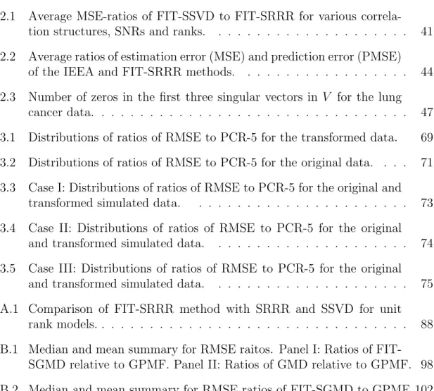
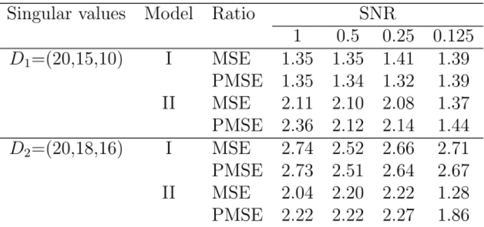
2.1 Average MSE-ratios of FIT-SSVD to FIT-SRRR for various correla-tion structures, SNRs and ranks. . . 41 2.2 Average ratios of estimation error (MSE) and prediction error (PMSE)
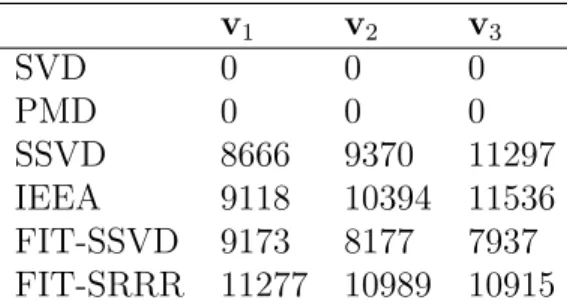
of the IEEA and FIT-SRRR methods. . . 44 2.3 Number of zeros in the first three singular vectors in V for the lung
cancer data. . . 47 3.1 Distributions of ratios of RMSE to PCR-5 for the transformed data. 69 3.2 Distributions of ratios of RMSE to PCR-5 for the original data. . . . 71 3.3 Case I: Distributions of ratios of RMSE to PCR-5 for the original and
transformed simulated data. . . 73 3.4 Case II: Distributions of ratios of RMSE to PCR-5 for the original
and transformed simulated data. . . 74 3.5 Case III: Distributions of ratios of RMSE to PCR-5 for the original
and transformed simulated data. . . 75 A.1 Comparison of FIT-SRRR method with SRRR and SSVD for unit
rank models. . . 88 B.1 Median and mean summary for RMSE raitos. Panel I: Ratios of
FIT-SGMD relative to GPMF. Panel II: Ratios of GMD relative to GPMF. 98 B.2 Median and mean summary for RMSE ratios of FIT-SGMD to GPMF. 102
1. INTRODUCTION
As high-dimensional data arises from various fields in science and technology, traditional multivariate methods need to be updated. Dimension reduction is im-portant in analyzing the high-dimensional data matrices, where low-rank matrix approximation and regularization techniques are of great interest. Principal compo-nent analysis (PCA) and reduced rank regression (RRR) are two of the most impor-tant multivariate statistical techniques that have seen major changes in recent years. In the modern approaches, particular attention is paid to improving the statistical performance and achieving fast computational efficiency. Given these goals, recent approaches aim at regularizing both the row and column factors of the low-rank ma-trix approximation by adopting the Lasso-type penalties. Thresholding is another powerful technique for regularizing the row and column factors without solving an optimization problem. This dissertation research covers two novel applications of the idea of thresholding: the thresholding reduced rank multivariate regression and the generalized PCA/singular value decomposition (SVD).
High-dimensional data matrices usually have structural dependencies where both the rows and columns are dependent. Ignoring these dependencies can lead to poor statistical performances. In this section, we first introduce the transposable data matrix with two-way dependencies and two real-data applications as the motivation for this research. We next review the classical dimension reduction tools for the low-rank matrix approximation in multivariate analysis: the singular value decom-position and the principal component analysis in Sections 1.2 and 1.3. These two approaches are central to the regularized low-rank matrix approximation methods. After introducing the Lasso-type regularization in Section 1.4, the literature review
for various regularization methods in the low-rank model and in the multivariate linear regressions are presented in Sections 1.5 and 1.6, respectively.
1.1 Transposable Data
Transposable data matrices are routinely encountered in fields such as economet-rics, bio-informatics, chemometeconomet-rics, network data, and so on. Such data matrices, where rows and columns are both dependent, have drawn much attention in re-cent statistical analyses. Recovering the true subspace or low-rank signal from the transposable data through low-rank matrix approximation is crucial in the statistical analysis.
For example, the macroeconomic data analyzed in Stock and Watson (2012) con-sisting of 144 U.S. macroeconomic time series for a total of 195 quarterly observations is a transposable dataset, because there are strong dependencies among feature vari-ables (columns) and temporal dependencies among observations (rows). To make accurate forecasting it is ideal to extract a parsimonious set of common factors from the data matrix. This idea is important and useful especially for datasets where the series are correlated and the number of observations are close to or less than the number of variables.
Another important example is the functional MRI (fMRI) data (Lindquist, 2008; Allen et al., 2013) that consists of measurements of brain images (columns) over time (rows) and exhibits spatial and temporal dependencies. Each pixel in the fMRI brain images corresponds to a measure of activation in the brain (Lazar, 2008). Finding major brain activation patterns is a primary analysis goal in the fMRI studies. It requires the algorithms to extract the important information from a mix of noise and signal, or a low-rank matrix approximation is desired.
the singular value decomposition and the principal component analysis, which are the fundamental methods for the low-rank matrix approximation.
1.2 The Singular Value Decomposition
The singular value decomposition (SVD), a fundamental conceptual and com-putational technique in linear algebra, has been used widely in the recent high-dimensional data situations for dimension reduction, data visualization, data com-pression, and information extraction by relying on its first few singular vectors (Golub and Van Loan, 1996).
LetY ∈Rn×q be a matrix, its SVD is of the form:
Y =U DV0 = q
X
i=1
diuivi, (1.1)
where the columns of U = [u1, ...,uq] ∈ Rn×q and V = [v1, ...,vq] ∈ Rq×q are the
left and right singular vectors, respectively. The matrices U and V are orthonormal with U0U =Iq, V0V = Iq and the matrix D ∈ Rq×q is a diagonal matrix with non-negative entries, called the singular values of Y. According to the Eckart-Young Theorem, for a given r, truncating the SVD gives the best rank-r approximation to a matrix Y. Let ||Y||F denote the Frobenius norm of the matrixY where ||Y||2F =
Pn i=1 Pq j=1y 2 ij =tr(Y0Y).
Theorem 1.2.1 (Eckart and Young, 1936) For anyr, the matrixY(r)=Pr
i=1diuivi
is the closest rank-r approximation to Y in the Frobenius norm,
Y(r)= arg min
rank(B)=r||Y −B||
2
F,
where di,ui,vi, i = 1, ..., r are the first r singular values and singular vectors of the
The Power method (Golub and Van Loan, 1996) is the most popular method for computing the SVD of a matrix, where a pair of left and right singular vectors is computed iteratively. For a matrix Y, it starts with an initial unit q-vector v(0) and
generates a sequence of unit vectors u(k) and v(k), k = 1,2, ...through the following
two steps until convergence:
(1). Updating u: u(k) =Yv(k−1)/||Yv(k−1)||, (2). Updating v: v(k)=Y0u(k)/||Y0u(k)||.
For u and v the unit vectors at convergence, the corresponding singular value is given by d =u0Yv. Then, the first rank-1 layer duv0 is subtracted from Y and the power method is applied to the residual matrix Y −duv0 to obtain the second pair of singular vectors, and so on.
An alternative to the power method is the idea of orthogonal iteration, which computes several leading left and right singular vectors ‘at once’ rather than a pair at a time (Golub and Van Loan, 1996). The orthogonal iteration method gener-alizes the power method from a vector to a subspace setup and achieves subspace orthogonalization through the QR decomposition. The QR decomposition is a de-composition of the matrix into an orthogonal matrix and a triangular matrix (Golub and Van Loan, 1996). For a matrix Y ∈ Rn×q, the orthogonal iteration is a stan-dard method for computing the subspaces spanned by its leading r singular vectors. Of course, for r = 1 the method reduces to the power method. It starts with an initial orthonormal matrix V(0) ∈Rq×r and generates sequences of orthonormal ma-trices U(k) ∈ Rp×r and V(k) ∈ Rq×r, k = 1,2, ... through the four steps in Figure 1.1 until convergence. For U and V the orthonormal matrices at convergence, their columns are the leading left and right singular vectors of Y, which are orthogonal by construction using the QR decomposition.
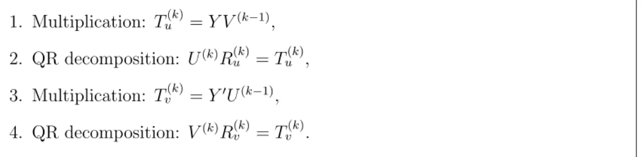
1. Multiplication: Tu(k)=Y V(k−1), 2. QR decomposition: U(k)R(k) u =Tu(k), 3. Multiplication: Tv(k)=Y0U(k−1), 4. QR decomposition: V(k)R(k) v =Tv(k).
Figure 1.1: The four key steps of the orthogonal iteration algorithm.
1.3 The Principal Component Analysis
The principal component analysis (PCA) is one of the most popular techniques in multivariate analysis, which is closely related to the SVD (Golub and Van Loan, 1996).
For a q-vector y = (y1, ..., yq)0, the PCA is to explain the population covariance matrix Σ of y through r linear combinations of y. Let V = [v1, ...,vr] ∈ Rq×r, then the linear combinations of y given by z1 = v10y, ..., zr = v0ry are called the principal components (PC) if the zi’s have the maximum variance and are uncorre-lated with each other. More precisely, the PCA computesV by solving the following optimization problems: v1 = arg max v v 0 Σvsubject to v0v= 1, v2 = arg max v v 0 Σvsubject to v0v= 1,v0v1 = 0, .. . vr = arg max v v 0 Σv subject to v0v= 1,v0vj = 0, for j = 1,2, .., r−1, (1.2)
which leads to the orthogonal matrix V with V0V = Ir. The vectors v1, ...,vr are called the loadings of the PCs, where the vi is the ith eigenvector of Σ and
var(zi) =var(v0iy) =d2i is its ith largest eigenvalue (Johnson and Wichern, 2007). For the sample data, the PCA of the centered data matrix Y ∈ Rn×q finds the eigen-decomposition of its sample covariance matrix S = n1Y0Y, an estimator of the population covariance Σ. The PCA provides the dimension reduction by forming the first r PCs of the originalq variables, where the PCs are possibly easier to interpret and visualize.
Since the SVD is usually used to solve the eigen decomposition problem, there is a direct relation between them where the loading matrix V of the PCs can be found by the SVD of Y = ˜UD˜V˜0 (Golub and Van Loan, 1996). More precisely,
Y0Y = ( ˜UD˜V˜0)0( ˜UD˜V˜0) = ˜VD˜2V˜0,
by using the orthogonality of the singular vectors ˜U and ˜V. By (1.1), the columns of ˜V corresponding to the first r largest singular values are the eigenvectors of Y0Y, which are the solutions for (1.2). Thus, the right singular vectors ˜V of Y are the same as the loading matrix of PCs of Y. This connection is crucial in introducing the sparse PCA and SVD algorithms in Sections 1.5 and 1.6.
For transposable matrices, the generalized principal component analysis (GPCA), first proposed by Escoufier (1977), is a natural generalization of the PCA. To high-light the key idea of the GPCA, we give a heuristic account on how to compute its loading matrix before introducing it more formally in Section 3.3.2. Given two symmetric positive-definite matrices Ω and Σ, the GPCA finds the loading matrix V = [v1, ...,vr] by maximizing the following criterion incorporating the matrices Ω
and Σ:
v1 = arg max
v v
0
ΣY0ΩYΣv subject tov0Σv= 1, v2 = arg max
v v
0
ΣY0ΩYΣv subject tov0Σv= 1,v0Σv1 = 0,
.. .
vr= arg max
v v
0
ΣY0ΩYΣv subject tov0Σv= 1,v0Σvj = 0, for j < r.
(1.3)
Different from the PCA, the loading matrix V of GPCA observes the generalized orthogonality constraint V0ΣV = Ir. The generalized principal components (GPC) are given byYΣv1, ..., YΣvr. The matrices Ω and Σ are closely related to the depen-dency structures of the transposable data discussed in details in the later sections.
Unfortunately, classical PCA and SVD encounter major problems in the high-dimensional data situations. The sample eigenvectors and singular vectors of PCA and SVD are not consistent estimators for their population counterparts (Johnstone and Lu, 2009; Fan and Lv, 2010). In addition, when eigenvectors and singular vectors of PCA and SVD have too many non-zero entries, they are hard to interpret and their use in practice could lead to misleading conclusions. Methods imposing sparsity or smoothness on the singular vectors and values have been shown to lead to consistency in high-dimensional settings (Johnstone and Lu, 2009). When the irrelevant entries in the eigenvectors and singular vectors are forced to zero, the statistical efficiency of the model and its interpretability are improved.
We review the Lasso-type regularization for the linear regression models in Section 1.4. We then illustrate its usage in the low-rank matrix approximation and the multivariate regression model in Sections 1.5 and 1.6, respectively.
1.4 Lasso-Type Regularizations
In this subsection, we review the method of least-squares estimation of the re-gression parameters with the Lasso-type (l1) penalties on the coefficients (Tibshirani,
1996).
Consider the linear model for the responsey∈Rn×1 and covariate X ∈Rn×p:
y=Xβ+e, (1.4)
whereβ∈Rp×1 is the coefficient vector andeis the noise. The ordinary least-squares
estimator of (1.4) ˆβ = (X0X)−1X0y does not perform well for the high-dimensional data situation when n ≤pas shown in Hastie et al. (2009).
The least absolute shrinkage and selection operator (Lasso) is one of the most popular approaches for selecting the most significant variables and estimating re-gression coefficients simultaneously. It penalizes the least-squares rere-gression using the l1 penalty on the coefficients and finds the Lasso solution ˆβ by minimizing the
objective function 1 2||y−Xβ|| 2 +λ p X j=1 |βj|, (1.5)
where λ denotes the tuning parameter controlling the sparsity of the coefficients. Note that λ= 0 corresponds to the least-squares estimator.
A number of innovative approaches are available to compute the Lasso solution. Two representative examples are the least angle regression (LARS) algorithm (Efron et al., 2004) and the coordinate descent algorithm (Friedman et al., 2008). The LARS algorithm starts with the variable which is most correlated with the response, and computes the whole solution path of the Lasso as the tuning parameter λ changes.
The coordinate descent algorithm solves (1.5) by minimizing over one βi at a time while the other β’s are kept fixed and cycles through the parameters βi, i= 1, ..., p, until convergence.
The Lasso regression is very popular, but has some drawbacks such as the bias problem (Fan and Li, 2001). There are several alternative Lasso-type penalty func-tions designed to fix these drawbacks. Zou (2006) proposed the adaptive Lasso with the weighted l1 penalty leading to the objective function
1 2||y−Xβ|| 2+λ p X j=1 wj|βj|,
where the weights are data-driven with wj = 1/|βˆj|γ, ˆβj the ordinary least-squares estimator and γ > 0. Zou and Hastie (2005) proposed the elastic net where the penalty is a linear combination of the l1 and l2 penalties. Given nonnegative λ1 and
λ2, the objective function for elastic net is given by
(1 +λ2)||Y −Xβ||2+λ1 p X j=1 |βj|+λ2 p X j=1 |βj|2,
which generalizes both the Lasso (λ2 = 0) and the ridge regression (λ1 = 0).
There are extensive research in this area where other penalized least-squares or likelihood methods with various types of regularizations have been developed. A representative but incomplete list of references is Fan and Li (2001), Yuan and Lin (2007), Zhao and Yu (2007) and Meier et al. (2008).
1.5 The Low-Rank Matrix Model
In this subsection, we review the regularization methods in low-rank matrix ap-proximation. To find low-rank signal from the data matrix Y ∈Rn×q, the following
setup (Yang et al., 2013; Allen et al., 2013) is considered
Y =B+E, (1.6)
where Y and B = U DV0 denote the data and the signal matrices, D the singular values, U and V the left and right factors, respectively.
The goal is to find a low-rank structure for the signal in the data matrix. IfY is the spatial-temporal fMRI data set described in Section 1.1, the rows would represent locations in the brain image and the columns point to the time effect. We present an overview of various methods for regularizing and computing the sparse singular vectors in U and V. There are two categories of algorithms: (i) the optimization-based sequential algorithms and (ii) the subspace iteration algorithms.
1.5.1 The Sequential Algorithms
Various regularization methods for computing the singular vectors have been pro-posed where the solutions are found sequentially through rank-one approximations. More precisely, the first rank-1 approximation is computed by imposing penalties on the vectors u and v. Then, the first computed layer duv0 is subtracted from Y and the procedure is repeated on the residual matrix. The first pair u and v, of U = [u1, ...,ur] and V = [v1, ...,vr], is found by minimizing the following objective function:
1
2||Y −duv 0||2
F +Pλ(u,v), (1.7)
with respect to the triplet (d,u,v), where λ is the tuning parameter andPλ(u,v) is a penalty function on u and v. Some penalty functions introduced in recent years are listed below.
1. The sparse PCA via regularized SVD algorithm in Shen and Huang (2008) and the sparse SVD (SSVD) algorithm in Lee et al. (2010) use the additive penalty function:
Pλ(u,v) = λu||u||1+λv||v||1,
where λu and λv are the tuning parameters for the left and right singular vectors, respectively. Using additive penalties with two penalty parameters allows different levels of sparsity on u and v.
2. The penalized matrix decomposition (PMD) algorithm proposed by Witten et al. (2009) relies on the following constraints/penalties:
||u||2 ≤1,||v||2 ≤1, Pu(u)≤cu, Pv(v)≤cv,
where Pu(·), Pv(·) are the Lasso or fused Lasso penalty, cu and cv are the cor-responding tuning parameters.
3. The sparse reduced rank regression algorithm (SRRR) in Chen et al. (2012a) applies multiplicative penalty on the singular vectors:
Pλ(u,v) = λ n X i=1 p X j=1 wij|duivj|,
whereui andvj are theith andjth entries of the vectorsuand v, respectively, and wij’s are data-driven weights as in the adaptive Lasso.
4. The penalized SVDs approach in Huang et al. (2009) uses a more general form of the multiplicative penalty function to regularize the singular vectors in the context of two-way functional data.
Unfortunately, the above regularization methods assume the entries of Y are i.i.d and ignore the row and column dependencies present in the transposable data. Ignoring the two-way dependencies in transposable data is known to lead to poor statistical performance (Efron, 2009; Allen and Tibshirani, 2010; Allen et al., 2013).
1.5.2 The Sequential Algorithm For Transposable Data
In Section 1.5.1, the low-rank matrix approximation problem was solved by min-imizing the Frobenius norm: ||Y −duv0||2
F. This loss function treats errors with equal weight and the covariances in the transposable data are ignored. To permit unequal weights according to the dependence structure of the data, Allen et al. (2013) proposed a generalized least-squares matrix decomposition (GMD) framework to di-rectly accounts for the known covariance matrices Ω and Σ. Define the transposable quadratic norm ((Ω,Σ)-norm) of a matrix A as ||A||2
Ω,Σ = tr(A
0ΩAΣ) to replace the Frobenius norm in finding the best low-rank approximation by minimizing the (Ω,Σ)-norm
||Y −duv0||2Ω,Σ , (1.8)
subject to the generalized orthogonality conditions
u0Ωu=v0Σv= 1. (1.9)
It turns out that for normally distributed data matrix defined next, the transposable quadratic norm (1.8) is proportional to the log-likelihood of the transposable data matrix Y ∈Rn×q.
distribu-tion (Gupta and Nagar, 1999) is defined and denoted by
Y ∼M Nn,q(M,Ω−1,Σ−1), (1.10)
where Ω−1,Σ−1 denote the rows and columns covariance matrices and M denotes the mean matrix of the data. The definition in (1.10) means that the vectorized Y is distributed as
vec(Y)∼Nnq(vec(M),Ω−1⊗Σ−1),
with a separable covariance structure where ⊗ denotes the Kronecker product and the vec operator forms a vector by stacking up the columns of a matrix.
It is easy to show that the log-likelihood function ofY can be written as:
l(Y|Ω−1,Σ−1)∝tr{(Y −duv0)0Ω(Y −duv0)Σ}=||Y −duv0||2Ω,Σ,
where the right hand side is (1.8).
To find the sparse GMD factors, Allen et al. (2013) proposed to regularize (1.8) using the Lasso penalty P(u,v) = λu|u|1 +λv|v|1 on u and v. However, their
algorithms are still sequential as in Shen and Huang (2008), Witten et al. (2009) and Lee et al. (2010), which lack orthogonality of the columns of U and V when r >1.
1.5.3 Subspace Iterations and FIT-SSVD
It is known that the sequential algorithms have expensive computation costs and cannot guarantee the orthogonality of the regularized singular vectors (Yang et al., 2013). Hence, a novel approach for low-rank approximation using the orthogonal iteration in (1.6) was proposed by Yang et al. (2013). Their fast iterative
thresh-olding for sparse SVDs (FIT-SSVD) algorithm computes the two subspaces spanned by the leading left and right singular vectors simultaneously which guarantees the orthogonality of the singular vectors. More precisely, the key ideas that distinguish the FIT-SSVD method from the earlier sequential methods are listed below:
1. the use of orthogonal iteration to compute the subspaces spanned by the first r singular vectors in U and V,
2. the use of thresholding to replace the smaller entries ofU andV by zeros, and novel, inexpensive ways of estimating the threshold levels,
3. sparse initialization by deleting the rows and columns of the data matrix with low signal.
Rather than solving the optimization problems in Section 1.5.1, the FIT-SSVD algorithm is based on thresholding. It adopts a thresholding function, like the familiar soft-thresholding
S(y, γ) =sgn(y)(|y| −γ)+,
the hard-thresholding
H(y, γ) = y1|y|>γ
or SCAD (Fan and Li, 2001), where γ is the threshold level. The threshold level γ is selected to be √2 logn motivated by the asymptotic results from the Gaussian sequence models (Johnstone, 2011) or using the idea of “m out of n” bootstrapping the data. These novel ways of estimating the threshold level avoid choosing tuning parameters by the computationally expensive cross-validation methods and hence
lead to fast computational performance. A detailed introduction of the FIT-SSVD is given in Section 2.2.1.
Selecting the threshold level in the FIT-SSVD algorithm relies heavily on the independence of the entries of a data matrix. Generalizations of the FIT-SSVD to account for the row-dependence are proposed in Section 2, where the correlations are incorporated in selecting the threshold levels.
1.6 Multivariate Linear Regression
In this subsection, we review the reduced rank regression (RRR), its connection to various multivariate methods and various ways to regularize the regression coefficient matrix.
Givennobservations on theq-vector of responsesyand thep-vector of predictors x, the multivariate linear regression model is
Y =XB+E, (1.11)
where Y = (y1, ...,yn)0 ∈ Rn×q, X = (x1, ...,xn)0 ∈ Rn×p and B ∈ Rp×q denote the responses, covariates and regression coefficients matrices, and E the noise matrix consists of iid normal random variables. Note that at least for a full-rank design matrix, X can be removed from (1.11) by left multiplying both sides by (X0X)−1X0 leading to
˜
Y = (X0X)−1X0Y = (X0X)−1X0XB+ (X0X)−1X0E.
It appears to be of the form (1.6), but with Y and E replaced by ˜Y = ˆBOLS = (X0X)−1X0Y and ˜E = (X0X)−1 X0E. This situation with the ˜E will be extensively studied in this dissertation.
The number of parameters inB can be quite large when both dimensions p and q are large, and its regularization is advisable when either dimension exceeds the sample size n. An early approach to regularization of B is the RRR (Anderson, 1951; Izenman, 1975) where one finds the least-squares estimate of B subject to the rank constraint rank(B) = r, for a given integer r. Hence, the coefficient matrix B = Θ1Θ2 can be written as a product of two lower dimensional matrices Θ1 ∈Rq×r
and Θ2 ∈ Rr×p of rank r. Thus, the RRR reduces the potentially large number of
parameters in B from pq to r(p+q) which is linear in p and q. Let the matrices X and Y be centered, given any positive-definite matrix W ∈Rq×q, the solution Θ1
and Θ2 of the RRR problem is computed by minimizing a weighted sum-of-squares
criterion
tr{(Y −XΘ1Θ2)0W(Y −XΘ1Θ2)}, (1.12)
which is of the form of (Ω,Σ)-norm, see Figure 1.2. Then, the solution is given by (Reinsel and Velu, 1998; Izenman, 2008)
Θ1 = Σ−XX1 ΣXYW1/2P = ˆBOLSW1/2P,
Θ2 = P0W−1/2,
where P = [p1, ..., pr] ∈ Rq×r and pi is the eigenvector corresponding to the ith largest eigenvalue of the matrix
where
ΣXX =Cov(X, X),ΣXY = ΣY X0 =Cov(X, Y),ΣY Y =Cov(Y, Y),
which are proportional to X0X, X0Y and Y0Y, since X and Y are centered.
The RRR problem provides a very general framework subsuming various widely used techniques in multivariate statistics, see Figure 1.2.
1. Setting W = I and Y = X, the (1.12) reduces to a PCA problem and have solutions Θ1 =P and Θ2 =P0, where P =V is the eigenvectors of ΣY Y as in Section 1.3. Thus, the RRR solves the PCA problem for data Y.
2. In the canonical correlation analysis (CCA) (Hotelling, 1935, 1936), the goal is to find vectors g and h such that the correlation corr(g0x, h0y) is maximized. Let G = (g1, ..., gr) ∈ Rp×r and H = (h1, ..., hr) ∈ Rq×r, the CCA is to find matricesGandHthat minimize all the eigenvalues of (Y H−XG)0(Y H−XG). It has been shown in Reinsel and Velu (1998) that by letting W = Σ−Y Y1 in (1.12), the solutions of the CCA are G= Θ1 and H = Θ02 as in the RRR.
3. The CCA setup can be reduced to the Fisher’s linear discriminant analysis (Fisher, 1936) if the response is a vector of binary variables.
4. The CCA setup can also be reduced to the correspondence analysis (Hirschfeld, 1935) if both the responses and the predictors are binary variables as shown in (Izenman, 2008).
There is a host of regression estimators that either regularize the weighted least-squares estimators (WLS) or regularize the likelihood function. In the literature, particular attention is paid to using the penalty on the singular values and singular
Figure 1.2: A diagram of RRR-related methods.
vectors of the coefficient matrix. The rank-r approximation of the coefficient matrix B is found using the SVD of B = Pr
i=1diuiv
0
i (Chen et al., 2012a). We show the details of the connection between the solution of (1.12) and the SVD in Section 3. Using the weighted Frobenius norm or the (Ω,Σ)-norm, the regularized RRR finds the minimizer of
||(Y −XB)W1/2||2F +Pλ(B) =||Y −XB||2I,W +Pλ(B),
where W denotes a weight matrix andPλ(B) is a penalty function on B or its SVD factors U, D andV. WhenW = Σ−Y Y1, where ΣY is the population covariance matrix
of the responseY andY ∼N(XB,ΣY Y), the above objective function is proportional to the regularized log-likelihood function:
l(Y|ΣY Y)∝tr{(Y −XB)0ΣY Y−1(Y −XB)}=||Y −XB||
2
I,Σ−Y Y1.
We list first those methods where penalties are imposed on the singular values of the coefficient matrix:
1. Yuan et al. (2007) proposed a nuclear norm penalized (NNP) least-squares estimator by setting Pλ(B) =λ||B||∗ = r X i=1 di,
where di(B) denotes the ith singular value of B. The NNP encourages sparse singular values, hence it performs dimension reduction and coefficient estima-tion at the same time. However, computing the estimates is very challenging in practice due to the nuclear norm constraint. Cai et al. (2010), Toh and Yun (2010) and Lu et al. (2012) have conducted extensive research to solve this optimization problem.
2. Bunea et al. (2011) proposed the rank selection criterion (RSC) by setting
Pλ(B) = λ r
X
i=1
I(di 6= 0),
where I(·) is an indicator function. It has low computational complexity com-pared to the NNP and has the explicit solution ˆB = (X0X)gX0Y V D−1H(D)V0, whereU DV0 is the SVD of the predictorX(X0X)gX0Y,H(D) =diag{diI(di > λ), i= 1, ..., r}. The RSC provides consistent estimators of the rank of the
co-efficient matrix when both n and pgo to infinite.
3. Dobrev and Schaumburg (2013) proposed the Tikhonov regularization of re-duced rank regression (TRRR) by setting
Pλ(B) =λ||R(Θ1Θ02)W 1/2||2
F =λ||Θ1Θ02|| 2
R0R,W,
subject to Θ01ΣXXΘ1 = Ir. Here, B = Θ1Θ02 and R is a pre-determined
ma-trix which may be chosen to differentially penalize certain directions in the parameter space. Its solution can be obtained by solving a generalized eigen-value problem |ΣXYWΣY X−ρ(ΣXX +λR0R)|= 0, where ρ is the generalized eigenvalue.
4. Chen et al. (2012b) proposed the adaptive nuclear norm penalization (ANN) by penalizing the mean (predictor) XB instead ofB,
Pλ(B) = λ r
X
i=1
widi(XB),
where di(XB) denotes the ith singular value of XB. It has the explicit so-lution ˆB = (X0X)gX0Y V D−1S
λw(D)V0, where U DV0 is the SVD of the pre-dictor X(X0X)gX0Y, Sλ(D) = diag{(di −λ)+, i = 1, ..., r}, where the
soft-thresholding operator acts on the singular values of the matrixXB. The ANN method directly tackles the prediction matrix approximation and imposes the sparsity on XB rather thanB. The selection of the tuning parameters {λ, w}
in the ANN are data-driven.
These regularized RRR approaches penalize the singular values of the coefficient matrix and encourage sparsity in the singular values and hence restricts the rank.
In order to account for the possible sparsity of the singular vectors, we list two representative methods below that enforce sparsity penalties on the singular vectors of the coefficient matrix.
1. Chen et al. (2012a) proposed the sparse reduced rank regression by setting
Pλ(B) = r X k=1 λk p X i=1 q X j=1 wijk|dkuikvjk|,
where uik, vjk are entries of uk and vk and wijk’s are the data-driven weights as used in the adaptive lasso. The iterative exclusive extraction algorithm is proposed to estimate B with sparse SVD structure starting from some initial consistent estimator ofB, e.g. the reduced rank least-squares estimator ˆBOLS =
Pr
l=1dˆluˆlvˆl0. They reduce the task of regularizing B into r parallel sparse unit rank regressions by decomposing the response matrix Y into r layers Yl = Y −X( ˆBOLS −BˆOLS,l), where ˆBOLS,l = ˆdluˆlvˆl0 and l = 1, ..., r, and solve the sparse regression of Yl’s on X with unit rank coefficient matrix.
2. Chen and Huang (2012) proposed a group lasso penalty of sparse reduced rank regression by setting Pλ(B) =λ p X i=1 |Θi.,1|,
whereB = Θ1Θ02, Θi.,1 is the ith row of Θ1, subject to condition Θ02Θ2 =Ir. It uses the idea of group lasso in Yuan and Lin (2007) and the numerical solution can be obtained through the subgradient or variational method.
Unfortunately, these regularization methods either simply assume the entries of noise E are iid distributed or assume E consists of independent columns, where the
dependencies among rows and columns as in the transposable data are ignored. The rest of the dissertation is organized as follows. We present our proposed novel regularization approach for the reduced-rank regression in Section 2, where its optimization problem is extensively discussed. We then extend our approach to the transposable data situation and incorporate the row and column dependencies in Section 3. Analyses of a micro-array data and a macroeconomic data follow the development of methodologies in each section. We conclude and discuss some future research topics in Section 4, and present the proofs and additional simulations in the Appendix.
2. REDUCED RANK MULTIVARIATE REGRESSION: THRESHOLDING AND OPTIMIZATION
Uncovering the meaningful relationship between the responses and the predic-tors is a fundamental goal in multivariate regression problems, which can be very challenging when data are high-dimensional. Dimension reduction and regularization techniques are applied extensively to alleviate the curse of dimensionality. It is desir-able to estimate the regression coefficient matrix by low-rank matrices constructed from its SVD. In this section, we integrate the reduced-rank regression approach with the regularization techniques and reduce such regression problems to sparse SVD problems for correlated data matrices and generalize the FIT-SSVD algorithm in Yang et al. (2013) to this situation. We also place Yang et al.’s algorithm in an optimization framework by introducing a specific bi-convex objective function. This enables us to study the large sample properties of the solution of the multivariate regression problem and establish consistency of the estimators as the sample size tends to infinity.
2.1 Background
There are very close and synergistic connections between the reduced rank mul-tivariate regression (Anderson, 1951; Izenman, 1975) and the SVD of its coefficient matrix (Reinsel and Velu, 1998; Yuan et al., 2007; Chen et al., 2012a). Consider the multivariate linear regression model
where Y, X and B denote the n ×q, n× p and p×q matrices of the responses, covariates and regression coefficients, and E the noise matrix which consists of iid normal random variables.
To reduce the potentially large number of parameters in B, the reduced rank regression (RRR) finds the least-square estimate ofB subject to the rank constraint rank(B) = r ≤ min(p, q). Its solution is known (Reinsel and Velu, 1998; Chen et al., 2012a) to relate to the low-rank approximation property of the SVD of B =
Pr
i=1diuiv
0
i as discussed in Section 1.6. Note that the special case of p = n and X =Ip leads to the model
Y =B+E, (2.2)
where the low-rank approximation ofB has been studied as a free-standing low-rank model in the recent literature of high-dimensional data analysis, see Section 1.5. However, it has been noted (Johnstone and Lu, 2009) that for high-dimensional data the classical SVD lacks good computational and statistical properties.
A regularized least-squares approach to the RRR proposed by Yuan et al. (2007) penalizes the sum of the singular values of the coefficient matrix, it encourages spar-sity in the singular values and hence restricts the rank of B. Unfortunately, this approach and its variants (Bunea et al., 2011) do not take into account the possi-ble sparsity of the singular vectors. Regularization of the singular vectors has been proposed by Shen and Huang (2008, p.123), Witten et al. (2009), Lee et al. (2010) and Allen et al. (2013) where the solution is found sequentially through rank-one ap-proximations of the data matrix Y in (2.2). More generally, Chen et al. (2012a) have introduced a regularized reduced rank regression method by considering a low-rank approximation to the ordinary least square estimate (OLS) of the coefficient matrix
in the multivariate regression (2.1) using an adaptive lasso penalty on the singular vectors ul,vl, l = 1,· · · , m. A notable drawback of this sequential approach is that the orthogonality of the singular vectors cannot be guaranteed.
A common feature of these sequential algorithms is that they provide solutions of certain penalized optimization problems. A novel non-optimization based iterative approach for low-rank approximation of high dimensional data in (2.2) is the fast iterative thresholding for sparse SVDs (FIT-SSVD) algorithm proposed by Yang et al. (2013). Unlike Shen and Huang (2008), Witten et al. (2009) and Lee et al. (2010) which compute singular vectors sequentially one at a time, the FIT-SSVD algorithm computes the two subspaces spanned by the leading left and right singular vectors using the idea of orthogonal iteration (Golub and Van Loan, 1996, Chapter 8) which guarantees the orthogonality of the singular vectors. More precisely, the key ideas that distinguish the FIT-SSVD method from the earlier sequential methods are the use of orthogonal iteration, thresholding and its novel sparse initialization, see Section 1.5.3. The theory and simulation studies in Yang et al. (2013) confirm that the FIT-SSVD algorithm is computationally much faster than the earlier sequential algorithms.
Unlike the sequential algorithms, the FIT-SSVD algorithm is neither motivated by nor based on solving optimization problems. In this section, our first contribution is to place the FIT-SSVD algorithm in an optimization framework. We introduce a suitable bi-convex objective function and an iterative algorithm to minimize it via closed form iterates. This setup enables us to study the large sample properties of the FIT-SSVD solution and establish consistency of the estimators as the sample size n tends to infinity. Our second contribution is to reduce the more general regression problem (2.1) to the low-rank model (2.2), recognize and deal with its correlated error by generalizing the FIT-SSVD algorithm to the correlated data situation. We
propose a fast iteratively thresholded sparse reduced rank regression (FIT-SRRR) algorithm which addresses the lack of orthogonality of the singular vectors in Chen et al. (2012a) and accounts for the correlation. The FIT-SRRR methodology allows the use of covariates and guarantees that the SVD layers are orthogonal. It makes effective use of the distribution of errors in finding the threshold levels and inherits all the good computational and statistical properties of the FIT-SSVD algorithm. Our simulation study and data analysis reveal the considerable gain when the dependence in the data is accounted for.
The rest of the Section 2 is organized as follows. In Section 2.2, after briefly reviewing the FIT-SSVD algorithm in Yang et al. (2013), we place it in an optimiza-tion framework. We develop in Secoptimiza-tion 2.3 the FIT-SRRR algorithm for the sparse reduced rank regression. We illustrate our methodology using simulations and real data in Sections 2.4 and 2.5, respectively. Section 2.6 concludes this section.
2.2 Thresholding for Sparse SVDs
In this subsection, we briefly review the FIT-SSVD algorithm and place it in an optimization setup by proposing a bi-convex objective function.
2.2.1 Overview
Recalling Section 1.2, the power method (Golub and Van Loan, 1996) is the most basic tool for computing the singular vectors of a matrix. Given an initial vector, it iteratively computes a pair of left and right singular vectors at a time. The alternative technique of orthogonal iteration computes several left and right singular vectors ‘at once’ and generalizes the power method from a vector to a subspace setup. It achieves subspace orthogonalization through the QR decomposition. A key step of the FIT-SSVD algorithm is based on the idea of orthogonal iteration.
vec-tors ofB withrorthonormal columns, the FIT-SSVD algorithm at the kth iteration applies multiplication toB andB0byV(k−1)andU(k)followed by thresholding. Then,
the QR decomposition of the thresholded matrices gives the orthonormal matricesU and V. It iterates according to the four steps in the Figure 2.1 until convergence.
1. Right-to-left Multiplication and Thresholding: U(k),thr =η(BV(k−1), γu), 2. Orthonormalization with QR Decomposition: U(k)Ru(k) =U(k),thr,
3. Left-to-right Multiplication and Thresholding: V(k),thr =η(B0U(k), γ
v), 4. Orthonormalization with QR Decomposition: V(k)R(k)
v =V(k),thr. Figure 2.1: The four key steps of the FIT-SSVD algorithm.
In Figure 2.1, the function η(.) is a pre-selected threshold function, like the fa-miliar soft-thresholding withη(y, γ) =S(y, γ) =sgn(y)(|y| −γ)+, hard-thresholding
η(y, γ) = H(y, γ) = y1|y|>γ or SCAD (Fan and Li, 2001), where γ is the threshold level. We work with the soft-thresholding function in the theoretical development here and discuss the other cases in the Appendix A.
Choosing the proper threshold levelγ requires the knowledge of the distribution of the noise E. In fact, selection of γ in Yang et al. (2013) relies heavily on the assumption of independence of the entries of the noise matrix. When this assumption is violated, we present a generalized FIT-SSVD algorithm in Section 2.3, which incorporates the dependence in the data.
2.2.2 An Objective Function Framework
Although the FIT-SSVD algorithm for model (2.2) as developed in Yang et al. (2013) is not optimizing-based, we introduce a suitable objective function in this
subsection and place it in an optimization-based framework. Consider minimizing the objective function,
Ψ(U, D, V) =||Y −U DV0||2 F +λu p X i=1 r X k=1 |uikdk|+λv q X j=1 r X k=1 |vjkdk|, (2.3)
over (U, D, V) subject to
U0U =Ir, V0V =Ir, (2.4)
where Y, U and V are p×q, p×r and q×r matrices, r≤m =min(p, q), andλu, λv are the regularization parameters. Note that (2.3) as an optimization problem with respect to matrices U, D, V is not bi-convex due to the two equality conditions onU and V in (2.4). We reduce it to a bi-convex optimization problem, following Witten et al. (2009) and Wittstock (1984, Definition 1.1) and finesse the equality conditions (2.4) and replace them by
(U0U −I)0,(V0V −I)0, (2.5)
where A 0 means that the matrix A is negative semi-definite. Now, it is evident that for V fixed, (2.3) subject to (2.5) is convex in U D, and similarly it is convex in V D for U fixed. Thus, the function Ψ(·) in (2.3) is bi-convex in U D and V D subject to (2.5). It can be minimized (Gorski et al., 2007) by iteratively minimizing the convex functions (2.6) and (2.7) below with respect to ˜U = U D and ˜V = V D
while keeping the other fixed: ||Y −U V˜ 0||2 F +λu p X i=1 r X k=1 |u˜ik|, (2.6) ||Y −UV˜0||2 F +λv q X j=1 r X k=1 |v˜jk|. (2.7)
Fortunately, the minimizers of (2.6) and (2.7) have closed forms as component-wise soft-thresholding operators acting on Y. Moreover, the minimizers ˜U(k) and
˜
V(k) in the kth iteration of (2.3) have the same form as those in the kth updating
steps U(k),thr, V(k),thr in the FIT-SSVD algorithm for certain threhsolding levels, see Figure 2.1. These observations are summarized in the following proposition and its proof is given in the Appendix A.
Proposition 2.2.1 (a)Given the data matrixY and model (2.2), the objective
func-tion Ψ(.) in (2.3) subject to conditions (2.5) is bi-convex and can be minimized by
alternatively minimizing (2.6)-(2.7) with respect to U ,˜ V˜.
(b) The solution U˜ of (2.6) for V fixed is the component-wise soft-thresholding
of Y V, i.e. S(Y V,1
2λu) = [S(Y V)ij, 1
2λu]i=1,...,n;j=1,...,r. Similarly, the solution V˜
of (2.7) for U fixed is S(Y0U,12λv), where S(A, λ) for a matrix A denotes
soft-thresholding every entry of A with threshold level λ.
(c) The FIT-SSVD algorithm is equivalent to iteratively minimizing (2.6)-(2.7) for
fixed λu, λv, and then obtaining the orthonormal matrices U and V through the QR
decompositions of their solutions.
Proposition 2.2.1 shows that the FIT-SSVD algorithm provides the solution for the estimator (U, V) of (2.3) subject to (2.5) through iteratively solving for the matricesU andV. Compared to the sequential algorithms in Lee et al. (2010),Witten et al. (2009) and Chen et al. (2012a), it is a matrix-based algorithm. It solves
for the matrices U and V directly as opposed to solving for their column vectors sequentially. Specifically, if the threshold levels γu, γv in the FIT-SSVD algorithm are set to be 12λu,12λv as in (2.3), then the soft-thresholding estimators of the kth iteration ˜U(k),V˜(k) in (2.6) and (2.7) are identical to the estimators U(k),thr, V(k),thr in the FIT-SSVD (Figure 2.1, Step 1 and 3).
An advantage of placing the FIT-SSVD algorithm in the optimization-based framework is that the asymptotic properties of its solution can be studied using the techniques developed for the Lasso-type objective functions (Knight and Fu, 2000; Zou, 2006; Chen et al., 2012a; Chen and Huang, 2012). We discuss the existence of a local minimum of (2.3) and the selection consistency of its solutions in the Appendix A.
2.3 The Generalized Thresholding for Sparse Reduced Rank Regression In this subsection, we reduce the multivariate regression model (2.1) to a low-rank model for a correlated data matrix, and then generalize the FIT-SSVD to the correlated data situation. The transformed model (2.9) below is the bridge connecting the regression problem to the low-rank model and the standard SVD problems. Compared to the FIT-SSVD algorithm the key changes in the FIT-SRRR are in selecting the threshold levels for correlated data and the separate updating of U and V, which no longer is symmetric in U and V due to the dependence in the rows of the data matrix.
The close connection between the FIT-SSVD and FIT-SRRR methodologies is explained by noting that at least for a full-rank design matrix, X can be removed from (2.1) by left multiplying both sides by (X0X)−1X0 leading to
It appears to be of the form (2.2), but with Y and E replaced by ˜Y = ˆB = (X0X)−1X0Y the least-square estimate ofB, and the transformed noise ˜E = (X0X)−1
X0E. However, the model (2.8) is more general than (2.2), since with
˜
Y =B+ ˜E, (2.9)
the columns of ˜E are iid Np(0, σ2Σ) where Σ = (X0X)−1 is known. Depending on the rank of the design matrix X, the following three cases are of interest:
I: X is orthonormal and X0X = I: Then, the proposed FIT-SRRR algorithm reduces to the FIT-SSVD algorithm of Yang et al. (2013). The latter will be used verbatim in computing the sparse SVD of the coefficient matrix B where
˜
Y =X0Y is used as the data matrix in the algorithm.
II: X has full column rank: Then, the entries of transformed noise ˜E in (2.9) are no longer iid, but row-wise dependent, so that the FIT-SSVD algorithm is not directly applicable, and it needs to be modified to account for the correlation. III: X is less than full-rank: In this case, there is no unique least square estimator of B in (2.8) because the Gram matrix X0X is singular. Some alternative estimators are the Moore-Penrose inverse (Bunea et al., 2011), and the ridge estimator. Throughout the Section 2, following Chen et al. (2012a, p. 8), the ridge estimator is used where a small positive constant = 10−4 is added to
the diagonal elements of the Gram matrix to make it invertible.
In the rest of this subsection, we describe the details of the FIT-SRRR algorithm, especially in updating U(k), V(k) and choosing the corresponding threshold levels.
1. Right-to-left Multiplication and Threshold U(k),thr =η( ˜Y V(k−1), γu), where γu is selected by Algorithm 1,
2. Orthonormalization with QR Decomposition: U(k)R(k)
u =U(k),thr,
3. Left-to-right Multiplication and ThresholdV(k),thr =η( ˜Y0U(k), γv), where γv is selected by Algorithm 2,
4. Orthonormalization with QR Decomposition: V(k)R(k)
v =V(k),thr. Figure 2.2: The four key steps of the FIT-SRRR algorithm.
2.3.1 Threshold Levels and Updating the U(k), V(k)
The goal of thresholding is to retain the entries of ˜Y with high signal and replace the others with zero. Due to row-dependence in the data matrix in (2.9), unlike the FIT-SSVD, finding U(k), V(k) in Step 1 and 3 in Figure 2.2 are no longer symmetric,
although they both require thresholding. We highlight this difference using some properties of matrix normal distributions (Gupta and Nagar, 1999). Recall that a random matrix Y (m×n) is said to have a matrix normal distribution and denoted asY ∼M Nm,n(M,Σ,Ω), whereM is the mean matrix and Σ,Ω denote the row and column covariance matrices. The following properties of linear transformations of matrix normal distributions are needed in the sequel.
Proposition 2.3.1 (a) Let Y ∼ M Nm,n(M,Σ,Ω) and a be a suitable vector, then
Ya∼Nm(Ma,(a0Ωa)Σ), and Y0a∼Nn(M0a,(a0Σa)Ω).
(b) If E˜ ∼ M Np,q(0, σ2Σ, Iq) as in (2.9), and u,v are suitable vectors of unit
norm, then the entries of Ev˜ ∼ Np(0, σ2Σ) are dependent, while those of E˜0u ∼
We discuss the details of selecting the threshold levels and the updating proce-dures for U(k), V(k) through their lth column u(k)
l ,v
(k)
l , l = 1· · · , r. To update U(k), letV(k−1) be the update ofV at the (k−1)st iteration andv(k−1)
l be its lth column. Right multiplying both sides of (2.9) by v(lk−1) and using the SVD ofB leads to the mean model,
˜
Yv(lk−1) =Bvl(k−1)+ ˜Ev(lk−1). (2.10)
For the moment, let γul be a threshold level used in (2.10). Then, [ ˜Yv
(k−1)
l ]thr, a thresholded version of the response vector, would serve as an estimator of the mean vector in (2.10). Repeating this procedure for all l = 1,· · · , r leads to the matrix [ ˜Y V(k−1)]thr, and the orthonormal matrixU(k)is obtained from its QR decomposition. From Proposition 2.3.1(b), since the noise ˜Ev(lk−1) in (2.10) is dependent with covariance matrix Σ, the universal threshold level (Donoho and Johnstone, 1994) used in Yang et al. (2013) is not applicable. Then, we need to modify the FIT-SSVD to account for the dependence and heterogeniety in (2.10). Johnstone and Silverman (1997) and Kovac and Silverman (2000) suggest more general thresholding methods for correlated and heteroscedastic noise. In brief, their methods view the entries of the noise vector ˜Evl(k−1) as independent heterogeneous random variables and ignore the correlation structure.
Berkner and Wells (1998, 2001) and Delouille et al. (2004) generalize the above thresholding methods by incorporating the correlations. More precisely, the threshold level γujl for the jth entry of the vector ˜Yv
(k−1)
l is selected as
where from Proposition 2.3.1(b), ˆσ2
ujl = ˆσ2σjj and σjj is thejth diagonal entry of Σ. The γul, following Berkner and Wells (2001), is given by
γul = p 2(1 +δ) log(p), (2.12) where δ = max j6=j0(|corr({ ˜ Yvl(k−1)}j,{Y˜v (k−1) l }j0)|),
is the maximum of the magnitudes of the correlations in ˜Yv(lk−1). We adopt this thresholding procedure for the correlated case in updating U(k), and summarize the
details in Algorithm 1.
Algorithm 1: Selection of the threshold level γul =gu( ˜Y , U(k−1), V(k−1),σ).ˆ Input:
1. Data matrix ˜Y, covariance matrix Σ for the rows of the noise matrix; 2. Previous estimators of the singular vectorsU(k−1), V(k−1);
3. An estimate of ˆσ. Output:
Threshold level vectorsγul for l = 1, ..., r.
1 ˆσ2ujl←σˆ2σjj, where σjj is the jth diagonal entry of Σ;
2 γul ←p2(1 +δ) log(p) where δ= maxj6=j0(|corr({Y˜v(k−1)
l }j,{Y˜v
(k−1)
l }j0)|);
3 γujl←σujlγul,ˆ j = 1, ..., p;
4 returnγul = (γu1l, . . . , γupl)0, l = 1, ..., r.
We update V(k) through its lth column v(lk), l = 1, ..., r. Right multiplying the transpose of both side of (2.9) by u(lk), it follows that
˜
where the entries of the vector ˜E0u(lk) are iid N(0, σ2u(k)0
l Σu
(k)
l ), see Proposition 2.3.1(b). Since the noises in (2.13) are uncorrelated, a theoretically sensible (though not actionable) threshold level for ˜Y0u(lk) would be γvl = E{||( ˜E0u(lk))||∞} (Yang et al., 2013, Section 2.4). We adjust their Algorithm 3 to obtain the threshold levels γvl, l = 1, ..., r for the regression setup. Since the SVD of the matrix B is assumed to be sparse, let Lu, Lv denote the index sets for U and V in which every element in a row is zero, and Hu, Hv be the complimentary sets of Lu and Lv. Then, after a reordering of the rows and columns of B (still denoted as B), it can be partitioned as, B =U DV0 = BHuHv BHuLv BLuHv BLuLv = BHuHv 0HuLv 0LuHv 0LuLv . | {z } p×|Hv| | {z } p×|Lv|
Using a compatible partitioning of X, (2.1) can be rewritten as,
Y = X11BHuHv 0 X21BHuHv 0 +E, (2.14) | {z } n×|Hv| |{z} n×|Lv|
where X11, X21 are the corresponding submatrices of X. Note that in our setting,
the (2,1)-block or the submatrix X21BHuHv in (2.14) is not a zero matrix as in Yang
et al. (2013, Section 2.4) and the pure noise part is a n× |Lv| matrix. Following Yang et al. (2013, Section 2.4), if the dimension of the pure noise is large enough, say, n|Lv| > pqlog(pq), we find the threshold level by using the rule of ”m out n”
bootstrap (Bickel et al., 1997). Otherwise, we use the universal threshold level
γvl = ˆσvl
p
2 log(q), (2.15)
where ˆσvl2 = ˆσ2ul(k)0Σu(lk), for l ∈ {1, ..., r}. The details of choosing the threshold level is presented in the Algorithm 2. Then, [ ˜Y0u(lk)]thr, a thresholded version of the response vector in (2.13), would serve as an estimator of the mean vector. Repeating this procedure for all l = 1,· · · , r leads to the matrix estimator [ ˜Y0U(k)]thr, where the orthonormal matrix V(k) is obtained from its QR decomposition.
Algorithm 2: Selection of the threshold level γvl =gv( ˜Y , U(k), V(k−1),σ).ˆ Input:
1. Data matrix ˜Y, covariance matrix Σ for the columns of the noise matrix; 2. Previous estimators of the singular vectorsU(k), V(k−1);
3. Pre-specified number M of bootstraps; 4. An estimate of ˆσ.
Output:
Threshold level γvl for l= 1, ..., r.
1 Subset selection: Lu ={i:ui(1k)=...=u(irk) = 0}, Lv ={j :v (k−1) j1 =...=v (k−1) jr = 0},Hu =Luc,Hv =Lcv; 2 if n|Lv|> pqlog(pq) then 3 for t in 1,· · ·, M do
4 Sample pq entries from the pure noise part in (2.14) and reshape them
into a matrix Z ∈Rq×p; 5 C = [C:1, . . . , C:r]←Z[Σ1/2U(k)]Hu ∈q×r; 6 Dt:←(||C:1||∞,· · · ,||C:r||∞) ∈R1×r ; 7 γvl ←median(D:l),l = 1, . . . , r; 8 else 9 γvl ←σˆvlp2 log(q), where ˆσvl2 = ˆσ2u(k) 0 l Σu (k) l ; 10 returnγvl, l = 1, ..., r.
2.3.2 Implementing the Algorithm
The FIT-SRRR algorithm is designed to inherit the statistical and computational properties of the FIT-SSVD algorithm. Its main steps are described in Algorithm 3, where the sub-algorithms for selecting the threshold levels for U and V are given in Section 2.3.1.
The initial orthonormal matrices U(0) ∈ Rp×r and V(0) ∈ Rq×r are chosen as in Yang et al. (2013) by first reducing the dimensionality of data matrix as in Johnstone and Lu (2009) and then computing its ordinary SVD. We stop the FIT-SRRR Algo-rithm after thekth iteration if the maximum distance between the successive iterates is small, i.e. max{||PU(k) −PU(k−1)||22,||PV(k−1) −PV(k−1)||22} is less than or equal to
a preselected = 10−8, where P
A =AA0 is a projection matrix for an orthonormal matrix A, and ||A||2 denotes the spectral norm of the matrix A.
2.4 Simulations
In this subsection, we use simulations to assess and compare the performance of the FIT-SRRR with the existing methods, and report the results in next two subsections. The first subsection compares the FIT-SRRR with the FIT-SSVD for correlated data matrices in model (2.2). The second compares the FIT-SRRR in the regression model (2.1) with the iterative exclusive extraction algorithm (IEEA) in Chen et al. (2012a) described in Subsection 2.4.2.
Throughout, the rank of the true underlying matrixB is assumed to be known. The parameters and setups are as the same as in the simulations in Yang et al. (2013) and Chen et al. (2012a), i.e. we keep their setups for the threshold func-tion, Huberizafunc-tion, bootstrap, cross-validation and initial values. In particular, for the FIT-SRRR, the bootstrap parameter M = 100 in Algorithm 2, the thresh-old function is the hard threshthresh-olding η(·) = H(·) in Algorithm 3, and ˆσ = 1.4826
Algorithm 3: The FIT-SRRR Algorithm. Input:
1. Data matrix ˜Y, covariance matrix Σ for the rows of the noise matrix; 2. Target rank r, and an estimate of ˆσ;
3. Thresholding functionη;
4. Algorithmsgu and gv to calculate the threshold levels γu, γv; 5. Initial orthonormal matricesU(0) ∈Rp×r, V(0) ∈Rq×r. Output:
Estimators ˆU =U(∞),Vˆ =V(∞).
1 repeat
2 Obtain the matrix U(k),thr ←[u1(k),thr, ...,u(rk),thr], where
u(lk),thr =η( ˜Yvl(k−1), γul) and γul =gu( ˜Y , U(k), V(k−1),σ) forˆ l = 1,· · · , r;
3 Orthonormalization with QR decomposition for U: U(k)Ru(k)←U(k),thr;
4 Obtain the matrix V(k),thr ←[v1(k),thr, ...,vr(k),thr] where
v(lk),thr =η( ˜Y0u(lk), γvl) andγvl =gv( ˜Y , U(k), V(k−1),σ) forˆ l = 1,· · · , r;
5 Orthonormalization with QR decomposition for V: V(k)Rv(k) ←V(k),thr;
6 untilConvergence;
7 returnEstimators Uˆ =U(∞),Vˆ =V(∞).
M AD(as.vector( ˜Y)) is a multiple of the median absolute deviation (MAD) of the data. The repetitions for each simulation are N = 1000 times.
2.4.1 The Low-Rank Model with Correlated Data
In this subsection, we consider the low-rank model (2.2) with correlated data. Yang et al. (2013) have compared the FIT-SSVD algorithm with several sequential sparse SVD methods, such as SSVD in Lee et al. (2010), PMD-SVD in Witten et al. (2009), and found it to outperform them in terms of estimation accuracy and computation cost. Hence, it suffices here to compare the FIT-SRRR with only the FIT-SSVD algorithm.
The following three covariance structures for Σ = (σij) of the correlated noise in model (2.2) are used to illustrate the effects of correlated error on the FIT-SSVD
algorithm and the proposed FIT-SRRR algorithm which is designed to account for the correlation. 1. Compound symmetry, CS. σij = σ2 if i=j, σ2γ if i6=j.
2. Auto Regression, AR(1).
σij =σ2ρ|i−j|, i, j ∈ {1,· · · , p},
3. Moving Average, M A(1).
σij = σ2 if i=j, σ2 θ 1+θ2 if |i−j|= 1,
where γ, ρ and θ are the parameters in CS, AR(1) and M A(1) structures, respec-tively.
We generate data matrices according to model (2.2) with covariance structures from the above list and set parameters γ, ρ and θ to the three levels: 0.1, 0.5, 0.9. We chooseσ2 so as to have four different levels of signal to noise ratio (SNR): 1, 0.5,
0.25 and 0.125, where the SNR is calculated following Chen et al. (2012a, Section 4) and Yang et al. (2013).
For the unit rank B, following the example in Lee et al. (2010) and Chen et al. (2012a), we let the signal B =duv0 be a 50×100 matrix (p= 50 andq = 100), with
d= 50 and
˜
u = (10,−10,8,−8,5,−5, rep(3,5), rep(−3,5), rep(0,34))0, ˜ v = (10,9,8,7,6,5,4,3, rep(2,17), rep(0,75))0, u = u˜ ||u˜||,v= ˜ v ||v˜||,
where rep(m, n) denotes a vector of length n, whose entries are all equal to m. For the rank-2B, we set B =P2l=1dlulv0l where
˜
u1 = (10,−10,8,−8,5,−5, rep(3,4), rep(0,40))0,
˜
u2 = (rep(0,40), rep(2,5), rep(−2,5))0,
˜ v1 = (10,9,8,7,6,5,4,3, rep(2,17), rep(0,75))0, ˜ v2 = (rep(0,80),5,4,3, rep(2,17))0, d1 = 40, d2 = 30, ul = ˜ ul ||u˜l|| ,vl = ˜ vl ||v˜l|| , l = 1,2.
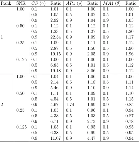
We measure the estimation accuracy of a method using the average mean-squared error ratio from the 1000 simulation repetitions, i.e. M SEi =||B −Bˆi||2F, and the average MSE-ratio is calculated by 10001 P1000i=1 M SEi,F IT−SSV D
M SEi,F IT−SRRR, where a value greater
than 1 indicates better performance of our proposed method.
Table 2.1 summarizes the results for the three correlation structures, four levels of SNRs and two ranks r = 1,2. It is evident that for the CS structure, the FIT-SRRR universally outperforms the FIT-SSVD. It enjoys a significantly lower level of mean-square errors than its counterpart, especially when the correlation parameter γ is large. It holds true for all levels of SNRs, and both ranksr = 1,2. For instance,