The Gender Pay Gap: Micro Sources and Macro Consequences

Munich Personal RePEc Archive

The Gender Pay Gap: Micro Sources and

Macro Consequences

Morchio, Iacopo and Moser, Christian

University of Vienna, Columbia University

11 May 2018

Online at

https://mpra.ub.uni-muenchen.de/99276/

The Gender Pay Gap:

Micro Sources and Macro Consequences

Iacopo Morchio† _{Christian Moser}‡

March 24, 2020

Abstract

We assess the sources and consequences of the gender pay gap using a combination of the-ory and measurement. We start by documenting three empirical facts. First, women are more likely than men to work at low-paying employers. Second, for women as for men, pay is not the sole determinant of workers’ revealed-preference rankings of employers. Third, both pay and the revealed-preference rank differ between women and men within the same employer. To inter-pret these facts, we develop an empirical equilibrium search model featuring endogenous gender differences in pay, amenities, and recruiting intensities across employers. The estimated model suggests that compensating differentials explain one fifth of the gender gap, that there are signif-icant output and welfare gains from eliminating gender differences, and that an equal-pay policy fails to close the gender pay gap.

Keywords: Worker and Firm Heterogeneity, Misallocation, Compensating Differentials, Discrimination,

Em-pirical Equilibrium Search Model, Linked Employer-Employee Data

JEL classification:E24, E25, J16, J31

∗_{We thank Daron Acemoglu, Jim Albrecht, Jorge Alvarez, Roc Armenter, Jesper Bagger, Erling Barth, Martin Beraja,} Mary Ann Bronson, Sydnee Caldwell, Rebecca Diamond, Rafael Dix-Carneiro, David Dorn, Niklas Engbom, Mikhail Golosov, Émilien Gouin-Bonenfant, Kyle Herkenhoff, Jonas Hjort, Philipp Kircher, Francis Kramarz, Kory Kroft, David Lagakos, Tzuo Hann Law, Rasmus Lentz, Ben Lester, Ilse Lindenlaub, Paolo Martellini, Guido Menzio, Magne Mogstad, Ben Moll, Giuseppe Moscarini, Andreas Mueller, Makoto Nakajima, Tommaso Porzio, Pascual Restrepo, Isaac Sorkin, Kjetil Storesletten, Coen Teulings, Gabriel Ulyssea, Gianluca Violante, and Susan Vroman for valuable comments and dis-cussions. We also thank attendants at the 2018 GEA Conference, 2019 AEA Annual Meeting, 2019 Search and Matching Network Conference, the 2019 Bank of Italy/CEPR/IZA Conference, the 2019 SED Annual Meeting, the 2019 NBER Sum-mer Institute, the 2019 Stanford SITE Workshop, the 3rd Dale T. Mortensen Centre Conference, the Boston Macro Juniors Conference, the 2020 Columbia Junior Micro Macro Labor Conference, and seminar participants at Columbia University, Boston University, CREST, Iowa State University, the University of Oslo, the University of Bristol, the University of Ed-inburgh, the University of Vienna, the Johannes Kepler University Linz, the Federal Reserve Bank of Philadelphia, and Temple University for helpful comments. Ian Ho and Rachel Williams provided outstanding research assistance. Moser gratefully acknowledges financial support from the Ewing Marion Kauffman Foundation and the Sanford C. Bernstein & Co. Center for Leadership and Ethics at Columbia Business School. Any errors are our own.

†_{University of Vienna. Email:[email protected].} ‡_{Columbia University. Email:[email protected].}

1

Introduction

During the past decades, the introduction of gender in economic theory and empirics has had a pro-found impact on studies of labor markets and the macroeconomy. A common thread in these studies is the robust empirical finding of a gender pay gap that is partly explained by gender imbalances in employment across different types of jobs. The goal of this paper is to identify the microeconomic sources of the gender pay gap and to assess its macroeconomic consequences.

We focus on two competing explanations for why women work in relatively lower-paid jobs. The first explanation pertains to compensating differentials: women may self-select into jobs with low pay but attractive amenities like work-schedule flexibility and paid parental leave. The second explanation pertains to gender-specific barriers to employment in desirable jobs: women may experi-ence more family-related labor market interruptions and certain employers may discriminate against them. The implications of the gender pay gap for output and welfare crucially depend on the relative importance of these two explanations.

In assessing the micro sources and macro consequences of the gender pay gap, we make three contributions. First, we use rich linked employer-employee data to establish novel facts on gen-der segregation, gengen-der-specific pay heterogeneity, and revealed-preference ranks across employers. Second, we develop and estimate a new empirical equilibrium search model featuring endogenous gender differences in pay, amenities, and recruiting intensities across employers. Third, we use the estimated model to decompose the empirical gender pay gap, to quantify the output and welfare gains from moving to an economy with no gender differences, and to evaluate the effects of a hy-pothetical equal-pay policy. In doing so, we provide the first estimates of output and welfare losses from firm-level gender misallocation.

To shed light on the gender dimension of employer heterogeneity, we analyze linked employer-employee records from Brazil between 2007 and 2014. The presence of a large gender earnings gap of around 14 log points makes it interesting in its own right to study the sources of gender inequality in a nation of over 200 million people. Such a study is feasible because Brazil’s remarkable data in-frastructure contains detailed information on gendered labor market outcomes, including workers’ educational attainment, occupation, contractual work hours, and employment histories with infor-mation on parental leaves.

We document that there is significant gender segregation across employers, with large differences in female employment shares across firms, even within sectors. To understand the link between

employer segregation and the gender pay gap, we estimate an empirical specification with gender-specific employer pay components developed byCard et al.(2016), building on the seminal two-way fixed effects (FEs) framework byAbowd, Kramarz, and Margolis(1999, henceforth AKM). Control-ling for unobserved worker heterogeneity, we find a gender pay gap of around 8 log points that is accounted for by gender-specific employer pay heterogeneity, with women sorting to lower-paying employers relative to men.

The extent to which empirical sorting patterns reflect compensating differentials can be inferred from revealed-preference employer rankings, which we construct separately by gender using the PageRank index (Page et al.,1998;Sorkin,2018). The PageRank is a network centrality measure that quantifies the attractiveness of employers based on the nature of worker flows between employers. Intuitively, higher-ranked employers poach many workers from other high-ranked employers and lose few workers to low-ranked employers. We use these estimates to establish three novel facts. First, the distribution of employment across employer ranks is similar for both genders. Second, the correlation between pay and employer ranks is positive, but more so for men than for women. Third, both within and across genders, there is significant heterogeneity in employer ranks conditional on pay.

To interpret these facts, we develop an empirical equilibrium search model featuring endoge-nous gender differences in pay, amenities, and recruiting intensities across employers. The model remains analytically tractable while accommodating several competing explanations for the gen-der gap, including employer productivity differences (Burdett and Mortensen,1998), gender-specific compensating differentials (Rosen, 1986), statistical discrimination (Arrow, 1971), and taste-based discrimination (Becker,1971). The model gives rise to gender-specific job ladders with several no-table equilibrium properties. The equilibrium wage equation is log-additively separable in a worker component and a gender-specific employer component, providing a microfoundation for the specifi-cation used inCard et al.(2016) and our own empirical investigation. Endogenous worker transitions may be associated with wage declines. Discriminatory employers may survive in equilibrium. Equi-librium spillovers of discrimination imply that even employers without regard for gender may end up offering different pay to men compared to women.

We identify four sets of gender-specific model parameters employer-by-employer using informa-tion on worker flows and employer pay across genders. We estimate gender-specific amenity values as the residual between employers’ relative pay and revealed-preference ranks in a set of bilateral comparisons. We use empirical worker flows by gender to obtain estimates of labor market

parame-ters, which map into heterogeneous degrees of statistical discrimination across employers. We com-pare the conditional equilibrium pay gap between coworkers of different genders within employers to identify parameters guiding a firm’s payoff from employing workers of each gender. Finally, we nonparametrically estimate employers’ gender-specific hiring costs from their empirical recruiting intensity among nonemployed workers.

The estimation results shed light on the microstructure of labor markets for men and women. Employer pay, ranks, and amenities are positively correlated within employers across genders. How-ever, employer ranks depend relatively more on pay for men but on amenities for women. We find evidence of compensating differentials for both genders. Employers’ preference for men over women increases with employer productivity, consistent withBecker(1971)’s idea that discrimination cannot survive among low-productivity firms with close-to-zero economic profits.

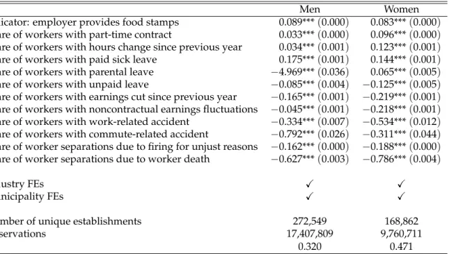
We link our structural estimates to relevant employer characteristics in the data. Women put rel-atively higher value on hours flexibility and parental leave benefits, while men are relrel-atively less averse to pay fluctuations and health risks. The empirical proxies for more woman-friendly employ-ers include higher routine-manual and nonroutine-cognitive-interpemploy-ersonal task intensities at work, higher female participation in general employment and top-paid positions, and having greater ac-countability to major financial stakeholders. These estimates speak to different reasons why some employers are not gender blind, including taste-based discrimination (Becker, 1971) and gender-specific comparative advantages related to “brain versus brawn” (Goldin,1992).

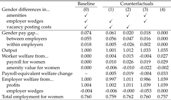
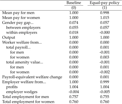
With the estimated equilibrium model in hand, we simulate a number of counterfactuals that shed light on the sources and consequences of the gender pay gap. We find that compensating differentials in the form of gender-specific amenities explain 1.3 log points (18 percent), employer tastes explain 5.4 log points (73 percent), and gender-specific hiring costs account for 5.6 log points (76 percent) of the gap. However, given the estimated structure of pay and nonpay characteristics across employers, closing the gender pay gap may or may not be welfare improving. We find that moving to an econ-omy without gender differences is associated with output gains of 3.5 percent and welfare gains of 3.3 percent, reflecting the current misallocation of talent across genders (Hsieh et al.,2019). In contrast, a hypothetical equal-pay policy is mostly output- and welfare-neutral, though it has redistributive effects.

Related literature. Several macroeconomic studies have focused on the drivers of trends in female

culture (Fernández et al.,2004;Fernández and Fogli,2009), technology (Greenwood et al.,2005;

Al-banesi and Olivetti, 2016), and information (Fogli and Veldkamp,2011; Fernández, 2013). Related

work has explored the implications of changes in female participation for economic growth (

Heath-cote et al.,2017;Hsieh et al.,2019), unemployment (Albanesi and ¸Sahin,2018), business cycles (Fukui

et al.,2019; Albanesi,2020), and declining dynamism (Peters and Walsh,2019). Whereas previous

work has focused on data at the aggregate, geographic, sectoral, or occupational level, our work highlights firm-level drivers of women’s employment and pay.

The firm is also a natural unit of analysis for studying productivity and factor input distortions in relation to macroeconomic outcomes (Restuccia and Rogerson,2008;Hsieh and Klenow,2009;Lentz

and Mortensen,2008;Bagger et al.,2014). Little prior work has connected firms’ gender composition

to aggregate output and welfare. If gender-specific barriers impede women’s relocation to higher-productivity firms, the gender pay gap may be associated with efficiency losses from misallocation of talent (Hsieh et al., 2019). By combining a rich equilibrium model with detailed microdata, we provide the first estimates of output losses from firm-level gender misallocation.

A burgeoning literature highlights firm heterogeneity in explaining empirical pay dispersion for otherwise identical workers based on AKM’s seminal contribution (Card et al.,2013;Goldschmidt

and Schmieder,2017;Alvarez et al.,2018;Card et al.,2018;Gerard et al.,2018;Song et al.,2018). We

build onCard et al.(2016), which estimates an empirical specification with gender-specific employer pay components on Portuguese data. Based on their specification, they decompose the gender gap in employer pay into sorting and rent sharing terms. The fundamental sources of the gender pay gap remain less well understood. By providing a microfoundation for their specification based on worker and firm optimization, our equilibrium model can rationalize gender-specific sorting and rent sharing patterns, and hence the empirical gender pay gap.

Our empirical equilibrium search model builds on the seminal framework byBurdett and Mortensen

(1998). Bontemps et al. (1999) and Bontemps et al.(2000) estimate variants of this framework with

heterogeneity in firm productivity. Other important extensions and empirical applications include

Postel-Vinay and Robin(2002),Cahuc et al.(2006),Moscarini and Postel-Vinay(2013),Meghir et al.

(2015),Engbom and Moser(2018),Heise and Porzio(2019), andBagger and Lentz(2018). In all these

models, firms are ex-ante heterogeneous in only one dimension, namely productivity. As a conse-quence, all workers agree on a common ranking of firms based purely on pay considerations. To rationalize our empirical facts on gender-specific employer pay and ranks, we develop and estimate a tractable framework with multiple dimensions of firm heterogeneity: productivity, gender

prefer-ences, amenity costs, and hiring costs.

Other models have addressed gender issues in the labor market. For example, Black (1995),

Bowlus (1997), Bowlus and Eckstein(2002), Albanesi and Olivetti(2009), Flabbi(2010),Gayle and

Golan (2011), and Amano-Patiño et al. (2019) study different forms of wage discrimination. It is

well known that discrimination is hard to empirically distinguish from unobserved productivity dif-ferences or compensating differentials. In our framework, linked employer-employee data with in-formation on worker transitions and coworker wages is necessary to separately identify employer preferences over gender from other dimensions of job heterogeneity.

Gender-specific compensating differentials à laRosen(1986) have been the empirical subject of

Goldin and Katz(2011,2016).Goldin(2014) andErosa et al.(2019) highlight flexibility as a job

char-acteristic with gender-specific value, which has been underlined by recent experimental evidence

(Mas and Pallais,2017, 2019;Wiswall and Zafar, 2017). Structural models of compensating

differ-entials have been developed and tested using survey data by Hwang et al. (1998), Lang and

Ma-jumdar (2004), Dey and Flinn(2005), Bonhomme and Jolivet (2009), andHall and Mueller (2018).

Like Taber and Vejlin (2016) and Xiao (2020), we exploit linked employer-employee data. Unlike

them, we identify gender-specific parameters employer-by-employer without relying on distribu-tional assumptions or indirect inference. Sorkin (2017),Lavetti and Schmutte(2017), and Lamadon

et al.(2019) also estimate firm-level amenity values from linked employer-employee data. Our

fo-cus, in contrast to theirs, is on gender. Sorkin(2018) combines PageRanks with a partial-equilibrium framework to study gender differences in pay and amenities, concluding that gender differences in the exogenous offer distribution explain a significant share of the gender pay gap. Our equilibrium framework provides a theory of endogenous gender differences in offer distributions, which is par-ticularly useful for our study the effects of an equal-pay policy.

Outline. The rest of the paper is structured as follows. Section2 introduces the data. Section 3

presents empirical facts. Section4develops the empirical equilibrium search model. Section5 out-lines the identification strategy. Section6presents estimation results. Section7conducts model-based counterfactuals. Finally, Section8concludes.

2

Data

2.1 Dataset and Variables Description

Dataset. Our main data source is theRelação Anual de Informações Sociais (RAIS)linked

employer-employee register administered by the Brazilian Ministry of Labor and Employment. Survey re-sponse by all tax-registered firms is mandatory and misreporting is deterred through threat of audits and fines. The data are available from 1985 onward, with coverage becoming near universal in 1994. Since 2007, the data contain detailed information on reasons and lengths of worker absences, includ-ing parental leaves. In 2015, the country entered a severe recession associated with a large drop in aggregate economic activity. Therefore, we focus on the eight-year period from 2007 to 2014. This leaves us with a large dataset of over 538 million employment records.

Variables. The data contain unique identifiers for workers and establishments.1 Although reports

are annual, we observe for each job spell the precise start and end dates, mean monthly earnings (henceforth “earnings”), and contractual work hours (henceforth “hours”). This allows us to avoid aggregation bias in classifying job-to-job transitions (Moscarini and Postel-Vinay,2018). Our baseline analysis uses earnings with flexible indicator controls for hours. However, for parts of our analysis we also construct hourly wages (henceforth “wages”) as earnings divided by the number of hours. Other key variables include gender in two categories, race in five categories, nationality in 37 cate-gories, educational attainment in nine catecate-gories, worker age in years, 5-digit sector codes with 672 categories, municipality codes with 5,565 categories, 6-digit occupation codes with 2,383 categories, and tenure in years. In addition, the data contain start and end dates of any absence from work, and information on the reason for absence. We exploit the full panel dimensions of the data going back to 1985 together with the tenure variable to impute actual (not just potential) formal-sector work experience in years.2

2.2 Sample Selection

We first restrict attention to male and female workers between the ages of 18 and 54 who worked at least one hour per week with earnings at or above the federal minimum wage. We then keep for each worker-year combination the highest-paid among all longest employment spells. Next, we

1_{All of our analysis is at the level of the establishment, which we intercheangably refer to as “employer” or “firm.”} 2_{The distinction between actual and potential experience is important in general but explains little of the empirical} gender pay gap—see Figure11in AppendixA.1.

iteratively drop singleton observations defined either by the combination of establishment identifier and gender, or by worker identifier. We also impose a minimum establishment size threshold of 10 nonsingleton workers per year on average.3 _{Finally, we require that establishments appear in our}

sample at least four out of the eight years. Together, the last two selection criteria ensure that we are dealing with a set of reasonably large and stable establishments for which pay policies and amenity values can be credibly estimated.

To separately identify worker and employer pay components, we follow Abowd et al. (2002) in constructing the largest connected set, where connections are formed through worker mobility between establishments over time. In the language of graph theory, there are two types of connected sets. Aweakly connected setis one in which each establishment is connected to another establishment through at least one incoming or outgoing worker. A strongly connected set is one in which each establishment is connected to another node through at least one incoming and one outgoing worker. For the AKM model to be identified, it is sufficient to restrict attention to weakly connected sets. However, to estimate revealed-preference ranks of employers using PageRanks requires restricting attention to strongly connected sets (Sorkin, 2018). Therefore, we restrict attention to the largest strongly connected set (henceforth “connected set”).

2.3 Summary Statistics

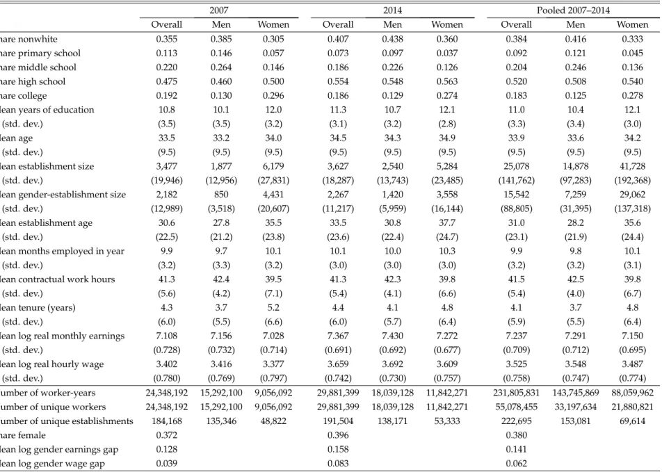
Table11 in AppendixA.2presents summary statistics on observations in the connected set in 2007, in 2014, and pooled across years 2007–2014.4 _{In the pooled sample, we have over 231 million}

worker-years, corresponding to over 55 million unique workers and over 222 thousand unique establish-ments. Around 38 percent of these observations are for women. The raw gender gap in earnings is around 14 log points and the gap in wages is around 6 log points. Compared to women, men are more likely to be nonwhite and hold at most a middle-school degree.5 _{Men are significantly younger,}

work at smaller and younger establishments, work more hours, and have lower tenure compared to women.6

3_{Following Sorkin(2018), nonsingleton workers are those who are observed at least one more time at a future date.} While the RAIS data cover only Brazil’s formal sector, the employer size restriction implies that the vast majority of informal establishments would be excluded from our analysis in any case (Ulyssea,2018;Dix-Carneiro et al.,2019).

4_{Also in AppendixA.2, we show the same summary statistics on the data before making sample selections and} restrict-ing the data to the connected set (Table12) and comparing the two samples (Table13).

5_{Since race information is missing for a significant share of observations, we report here the conditional mean.} 6_{In Brazil, full-time employment involves either 40 or 44 hours of work per week, depending on the employer.}

3

Employer Heterogeneity and the Gender Gap

A classical Mincerian analysis of the gender gap in pay is presented in Appendix B.1. Standard Mincerian controls only partly explain the empirical gender gap. Thus, building on AKM’s seminal contribution, we investigate the role of employer heterogeneity in relation to the gender gap.

3.1 Gender Segregation Across Employers

Women make up 38 percent of Brazil’s formal sector employment over the period 2007–2014. How-ever, women are highly segregated across employers, even within industries. Figure1shows a his-togram of female employment shares in 2014. Around 28 percent of establishments have less than 10% women among their workforce. In contrast, if women were equally distributed across employ-ers, we would see a single bar of height 10 in the category 30–40%.

Figure 1. Histogram of female employment shares, 2014

0 1 2 3 4 5 6 7 8 9 10 Density 0.0 0.1 0.2 0.3 0.4 0.5 0.6 0.7 0.8 0.9 1.0 Female employment share

Overall

Source:Authors’ calculations based on RAIS.

We show in AppendixB.2that gender segregation is a robust empirical phenomenon over time (Figure12), within sectors (Figure13), and across different employer sizes (Figure14). Figure15 in AppendixB.3shows that employment levels of men and women within establishments are positively but imperfectly correlated. In Appendix B.4, we quantify the degree of gender segregation across employers by defining and estimating an employer segregation index, which we find to be higher than analogous indices estimated across industries, occupations, or states.

3.2 Quantifying Employer Pay Heterogeneity

To understand the link between employer segregation and the gender pay gap, we estimate a wage equation with gender-specific employer pay components developed byCard et al.(2016), building on the seminal two-way FEs specification by AKM. This allows for the possibility that a given employer has two pay policies—one for each gender. Formally, we model earnings of individual i in year t working at establishmentj= J(i,t), denotedyijt, as

yijt= Xitβ+αi+1[genderi = M]ψMj +1[genderi =F]ψFj +εijt, (1)

whereXitis a vector of gender-specific worker characteristics including a set of restricted

age dummies as well as dummies for hours, occupation, tenure, actual experience, and education-year combinations,αiis a person FE,ψjMandψFj are the male and female employer FEs, respectively,

andεijtis a residual term.7 By including a set of person FEs, this specification controls for selection of

men and women across establishments based on unobserved time-invariant worker characteristics such as ability. In estimating equation (1), our main focus is on estimates of the gender-specific employer FEs,ψM_j andψF_j.

As is the case in all two-way fixed models, at least one normalization must be made regarding the intercept or mean of the employer FEs versus the person FEs. In our case, the model with gender-specific employer FEs requires two normalizations—one for each gender. Consistent with the the-oretical model presented later, we followCard et al.(2016) and Gerard et al.(2018) in normalizing the employer FEs of both genders to be of mean zero in the restaurant and fast-food sector, which, arguably, is populated by low-surplus employers.8

We now turn to our main object of interest in equation (1), namely the gender-specific employer FEs.9 _{Panel (a)of Figure 2 plots the distribution of employer FEs by gender. The distribution for}

women has visibly lower mean and lower variance than that for men. Panel(b)of the figure shows the distribution of within-employer differences in FEs for dual-gender establishments. The distribu-tion is relatively dispersed compared to its mean of around 2 log points.

7_{To identify age, time, and worker FEs simultaneously, we restrict the age-pay profile to be flat around ages 45–49,} which is approximately consistent with empirical raw-earnings profiles. See AppendixB.5for details.

8_{For robustness, we experimented with alternative normalizations for gender-specific employer FEs. Separately, we} have repeated our analysis based on a wage equation without worker FEs, making the normalization redundant.

9_{In AppendixB.5, we present auxiliary results relating to the AKM equation, including estimated gender-specific hours} FEs (Figure16), occupation FEs (Figure17), actual-experience FEs (Figure18), tenure FEs (Figure19), education-year FEs (Figure20), and education-age FEs (Figure21).

Figure 2. Predicted AKM employer FEs for women and men (a) Gender-specific employer FE distributions

0.0 0.5 1.0 1.5 2.0 2.5 3.0 3.5 Density −1.0 −0.8 −0.6 −0.4 −0.2 0.0 0.2 0.4 0.6 0.8 1.0

Gender−specific AKM employer FE

Men Women

(b) Gender-specific employer FE distributions

0 1 2 3 4 5 6 7 8 Density −0.5 −0.4 −0.3 −0.2 −0.1 0.0 0.1 0.2 0.3 0.4 0.5

AKM employer FE gap (male − female)

Source:Authors’ calculations based on RAIS.Note:Dashed vertical line shows mean of the distribution.

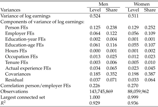
Table1shows a log-earnings variance decomposition.10 _{Men have a slightly higher variance of}

log earnings, with 52.4 log points compared to 51.1 log points. For both genders, the largest vari-ance component is due to estimated worker FEs, accounting for 24 percent for men and 25 percent for women. Employer FEs account for 12 percent of the variance of earnings for men and 11 per-cent for women. The positive covariance terms are primarily attributed to the covariance between worker and employer FEs, education-age and employer FEs, and actual experience and employer FEs. The correlation between person and employer FEs is around 23 percent for men and 27 percent for women. For each gender, the largest connected set spans close to the full data. Finally, around 93 percent of the variation in log earnings is explained by the model.

10_{To be precise, Table 1presents plug-in estimators of the variance components. In ongoing work, we are adapting} the leave-one-out estimator byKline et al.(2019), which implements a jackknife bias correction for limited-mobility bias

Table 1. Variance decomposition based on gender-specific employer FEs model

Men Women

Variances Level Share Level Share Variance of log earnings 0.524 0.511

Components of variance of log earnings:

Person FEs 0.125 0.238 0.129 0.252 Employer FEs 0.064 0.122 0.056 0.109 Education-year FEs 0.002 0.004 0.001 0.001 Education-age FEs 0.061 0.116 0.055 0.107 Hours FEs 0.000 0.001 0.001 0.002 Occupation FEs 0.013 0.025 0.012 0.023 Tenure FEs 0.003 0.006 0.005 0.010 Actual experience FEs 0.034 0.065 0.023 0.045 Covariances 0.185 0.352 0.198 0.387 Residual 0.037 0.071 0.033 0.064 Correlation person/employer FEs 0.226 0.270

Observations 143,745,869 88,059,962 Largest connected set 1.000 0.999

R2 0.929 0.936

Source:Authors’ calculations based on RAIS.Note:Variance components based on earnings equation (1).

3.3 Between vs. Within-Employer Pay Differences

Our focus from here on will be on differences in the gender-specific employer components (hence-forth “gender gap”). Using a Oaxaca-Blinder decomposition, we can write the gender gap as

γe ≡E_i,th_ψM J(i,t) genderi= M i −E_i,th_ψF J(i,t) genderi=F i =E_i,t h

ψM_J(i,t)−ψF_J(i,t)genderi= M

i

| {z }

within-employer gender pay gap

+E_i,t h ψF_J(i,t)genderi= M i −E_i,t h ψF_J(i,t)genderi=F i | {z }

between-employer gender pay gap

(2) =E_i,th_ψM J(i,t)−ψFJ(i,t) genderi=F i | {z }

within-employer gender pay gap

+E_i,th_ψM J(i,t) genderi= M i −E_i,th_ψM J(i,t) genderi=F i | {z }

between-employer gender pay gap

. (3)

Equations (2) and (3) are two alternative decompositions of the total gender gap,γe, into two terms.

Thewithin-employer pay gaporpay-policy componentis the mean difference in gender-specific employer FEs weighted by the distribution of men and women, respectively. It reflects differences in pay be-tween women and men at the same establishment. Thebetween-employer pay gaporsorting component is the difference between genders in mean male-employer FEs and female-employer FEs, respec-tively. It reflects differences in pay between men and women due to their different allocations across

establishments.11

Figure22in AppendixB.6graphically illustrates estimates of the two components of the decom-positions in equations (2) and (3). Results of the decomposition are shown in Table2. Out of the total gender pay gap of 8.4 log points, 24 (5) percent are attributed to the pay-policy component in Decomposition 1 (2). The remainder is attributed to the sorting component. This evidence suggests that women systematically work at lower-paying employers compared to men.

Table 2. Oaxca-Blinder decompositions of the gender pay gap due to employer heterogeneity Pay-policy component Sorting component Gender pay gap Level Share Level Share Decomposition 1 0.084 0.020 0.241 0.064 0.759 Decomposition 2 0.084 0.004 0.047 0.080 0.953

Source: Authors’ calculations based on RAIS.Note: Decompositions 1 and 2 correspond to equations (2) and

(3), respectively.

3.4 Life-Cycle Patterns and Event Study Analysis around Parental Leaves

An obvious candidate factor that may be behind some of the hitherto documented patterns is related to childbirth. In AppendixB.7, we study life-cycle patterns of employer pay by gender and parental status. In Appendix24, we conduct an event study analysis around childbirth (as proxied by parental leave) following Kleven et al. (2016). While we find significant gender gaps in participation and earnings associated with childbirth, our analysis suggests that firm pay heterogeneity isnotthe only, or even a very important, factor behind these gaps.

3.5 Revealed-Preference Employer Rankings

To what extent does the gender pay gap reflect a gender utility gap? To answer this question, one must take into account both pay and nonpay characteristics of jobs for both genders. To this end, we estimate gender-specific revealed-preference rankings of employers using the PageRank index. The PageRank is a network centrality measure developed by Page et al.(1998) to rank websites for the web search engine Google and first used in an economic context bySorkin(2018).

In a labor market context, the PageRank is defined as follows. Letg ∈ {M,F}index a worker’s gender, let j ∈ Jg _{= {j}

1,j2, . . . ,jNg}index a set of Ng gender-specific employers, and let t ∈ T 11_{Note that the sorting component is invariant to the choice of the normalization of gender-specific employer FEs.} Coin-cidentally, this will be the main object of interest in our study. The pay-policy component, on the other hand, depends on the normalization of men’s relative to women’s employer FEs.

index time. We denote byng_j,j′_,t the number of workers of gendergtransitioning from employer jto

employer j′ at timet, byng_j,j′ = ∑_t∈T n g

j,j′_,t the time aggregation of gender-specific flows between the

two employers, and byng_j,. = ∑_j′ng_j,j′ the number of workers of gendergflowing out from employer

j. LetBg(j) =nj′ :ng_j′_,j ≥1 o

denote the set of employers who have ever lost a worker of gendergto employerj. Letd∈[0, 1]be a damping factor. ThePageRank index,sg(j), is a probability distribution over all employersj∈ Jg_{such that}

sg(j) = 1−d Ng +d

∑

j′_,. is a weight equal to the share of worker flows from employerj′ to employer

jas a fraction of all worker flows from employer j′. Intuitively, employers with a high PageRank index poach many workers from other employers with high PageRank indices and lose few workers to other employers with low PageRank indices. The damping factordrepresents the weight on the poaching term in a convex combination with equal employer weights. Based on PageRank indices, we compute gender-specificPageRanks rg_{(j)for every employer j∈ J}g_{as the rank of the PageRank}

indices, with the lowest rank normalized to 0 and the highest rank normalized to 100.

Interestingly, the PageRank index represents the asymptotic share of time a representative worker (“random surfer”) who switches jobs by following the network of empirical worker flows would spend at a given employer. FollowingSorkin(2018), we choose as damping factord=1 in all our ap-plications. By estimating PageRank indices on the strongly connected set, we avoid absorbing states (“rank sinks”), in which a worker could get indefinitely stuck at an employer. This interpretation of the PageRank index is particularly close to the definition of an employer rank in a large class of on-the-job search models, including the one we develop. Note also that an employer’s PageRank does not directly depend on its pay or size. Indeed, in computing PageRanks, we did not use any information on worker wages or the number of workers at any employer.

Based on equation (4), we compute employer PageRanks separately by gender.12 _{We now}

estab-lish three facts relating to employer heterogeneity in pay and ranks within and across gender.13

12_{In AppendixB.9, we show that the resulting PageRanks are strongly but imperfectly correlated with gender-specific} employer FEs in pay. PageRank estimates are also strongly but imperfectly correlated with two other popular employer rank measures, namely the poaching rank (Moscarini and Postel-Vinay,2008;Bagger and Lentz,2018) and the net poaching rank (Haltiwanger et al., 2018;Moscarini and Postel-Vinay, 2018). An advantage of the PageRank over the other two rank measures is that it uses more information per worker transition in constructing an employer ranking, which reduces spurrious misclassifications of employer ranks.

13_{For the remainder of this section, we will study gender-population-weighted estimates of the unweighted PageRanks} as described above. Note that PageRanks are not restricted to have any particular mean value (e.g., 50) by construction

Fact 1. While the gender gap in pay ranks is 4.4 percentiles, that in employer ranks is 0.7 percentiles.

Figure3compares the employment distributions of men and women across pay ranks and across employer ranks. Panel(a)shows employment is weakly positively related to pay for both genders. Panel(b), on the other hand, shows that employment is strongly related to employer ranks for both genders. Furthermore, the rank-based employment distribution of women looks relatively more sim-ilar to that of men than it does for the pay-based employment distribution. Women’s mean employer pay rank is 53.9 while men’s is 58.3, implying a gender gap in pay ranks of 4.4 percentiles. On the other hand, women’s mean employer rank is 73.7 while men’s is 74.4, implying a gender gap in employer ranks of 4.4 percentiles.14

Figure 3. Densities over pay ranks and employer ranks, by gender (a) Pay ranks

0.00 0.01 0.02 0.03 0.04 0.05 Density 0 10 20 30 40 50 60 70 80 90 100

Gender−specific pay rank

Male pay ranks Female pay ranks

(b) Employer ranks 0.00 0.01 0.02 0.03 0.04 0.05 Density 0 10 20 30 40 50 60 70 80 90 100

Gender−specific employer rank

Male employer ranks Female employer ranks

Source:Authors’ calculations based on RAIS.

Fact 2. Mean employer ranks are steeper increasing in pay ranks for men than for women.

Figure 4 suggests that employer ranks are positively related to pay ranks for both men and women. However, the gradient is steeper for men than for women, especially in the bottom half of employer pay ranks. This means that there exist low-paying jobs that are at the same time rela-tive attracrela-tive for women, and that this is less so the case for men. Therefore, for men compared to women, pay is relatively more important in their overall evaluation of an employer’s rank.15

Fact 3. There is significant heterogeneity in employer ranks conditional on pay within and across genders.

since the PageRank estimation is independent of the cross-sectional employment distribution. 14_{Note, however, that this does not rule out a utility gap between genders.}

15_{AppendixB.10presents several robustness checks. Figure27shows the relationship between employer ranks and pay} ranks across sectors. Table17shows that this fact is not driven by sectoral or geographic differences. Table18shows that this fact is consistent with the dynamics of pay for different worker transitions across employer ranks.

Figure 4. Employer rank and pay, by gender 0 10 20 30 40 50 60 70 80 90 100

Mean gender−specific employer rank

0 10 20 30 40 50 60 70 80 90 100

Gender−specific employer pay rank

Men Women

Source:Authors’ calculations based on RAIS.

Figure5shows that there is significant dispersion in employer ranks conditional on pay for men in panel(a)and for women in panel(b). This suggests heterogeneity in nonpay characteristics of em-ployers.16 _{For both men and women, ranks are relatively more dispersed at low-pay employers than}

at high-pay employers. This suggests that establishments with high pay are also high in utility. This is consistent with either their pay being high enough to compensate for their level of (dis-)amenity, or alternatively their amenities being high on top of their high pay.17

Figure 5. Percentiles of employer rank distribution conditional on pay ranks, by gender (a) Men 0 10 20 30 40 50 60 70 80 90 100

Percentiles of male employer ranks

0 10 20 30 40 50 60 70 80 90 100

Percentiles of male pay

P10 P25 P50 P75 P90 (b) Women 0 10 20 30 40 50 60 70 80 90 100

Percentiles of female employer ranks

0 10 20 30 40 50 60 70 80 90 100

Percentiles of female pay

P10 P25 P50 P75 P90

Source:Authors’ calculations based on RAIS.

16_{Figure30in AppendixB.11shows that the standard deviation of employer ranks is similarly decreasing in employer} pay ranks for men and women.

17_{AppendixB.11shows that the same qualitative conclusions apply when, for robustness, we compare employer ranks} across pay ranks by industry for women (Figure28) and for men (Figure29).

Figure6 shows that there is also significant within-employer between-gender dispersion in pay ranks in panel(a)and in employer ranks in panel(b). Pay and employer ranks are strongly positively correlated within employers across genders. This is consistent with the idea that an employer’s pro-ductivity and amenities, such as its location and certain benefit policies, are partly shared by its male and female workers. Cross-gender employer ranks are also relatively more dispersed than cross-gender pay ranks. This may reflect that productivity (e.g., technology or management practices) is shared more freely across genders compared to valuations of certain amenities (e.g., hours flexibility or parental leave policies). Finally, men and women closely agree on their rankings of top employers, both in terms of pay ranks and employer ranks, but less so for lower-ranked employers.18

Figure 6. Female vs. male employer characteristics (a) Pay 0 10 20 30 40 50 60 70 80 90 100

Percentiles of female pay

0 10 20 30 40 50 60 70 80 90 100

Percentiles of male pay

P10 P25 P50 P75 P90 (b) Ranks 0 10 20 30 40 50 60 70 80 90 100

Percentiles of female employer rank

0 10 20 30 40 50 60 70 80 90 100

Percentiles of male employer rank

P10 P25 P50 P75 P90

Source:Authors’ calculations based on RAIS.

4

Model

Addressing the above empirical facts requires a structural model with the following ingredients. First and foremost, the model must allow for an employer’s revealed-preference rank to differ from its pay rank. To rationalize this, workers in the model value an employer’samenitiesin addition to pay. Second, the model must generate differences in pay and amenities across employers. To ratio-nalize this, the labor market is modeled as frictional. Third, the model must admit gender differences in pay, revealed-preference ranks, and employment within the same employer. To rationalize this, 18_{For robustness, AppendixB.11shows the same relation between female and male pay ranks by industry (Figure31)} and that between female and male employer ranks by industry (Figure32). The same qualitative conclusions apply within each of the industries.

employers in the model post gender-specific wages, amenities, and job vacancies. We combine these ingredients in an equilibrium model of the labor market.

4.1 General Environment

A measure 1 of workers and measureEof firms meet in a continuous-time frictional labor market.

4.2 Workers

Workers are infinitely lived, risk neutral, and discount the future at rateρ. They permanently differ

in abilitya∈ [a,a]and genderg ∈ {M,F}with measureµa,gsuch that∑g=M,F´aµa,gda =1. At any

point in time, they find themselves either employed or nonemployed.19

Job search. While nonemployed, workers receive flow utilityba,gand engage in random job search

within segmented labor markets by worker type. Search is random in the sense that workers cannot direct their search to specific firms. Labor markets are segmented in the sense that workers search for jobs in a market specific to their type. While employed, workers receive flow utilityx=w+πequal

to the sum of their wage,w, and job amenity value,π. Employed workers also engage in on-the-job search within the same segmented markets.

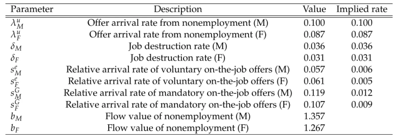
As a result of job search, workers receive regular job offers with arrival rate λu

a,g from

nonem-ployment and with rateλea,gfrom employment. While regular on-the-job offers admit free disposal,

workers also receive mandatory on-the-job offers (sometimes termed a “Godfather shock,” or an of-fer one can’t refuse) at rateλGa,gin both employment states. We think of the latter as capturing, among

other things, spousal relocation problems and other idiosyncratic reasons for switching jobs. We will writeλea,g=sea,gλua,gandλGa,g =sGa,gλua,g, wheresea,gandsGa,gare the relative search intensities of regular

and mandatory on-the-job search, respectively.

A job offer is an opportunity to work at some firm with associated wage wand amenity value

π, drawn from a distribution ˜F(w,π), which workers take as exogenous but which is determined endogenously through firms’ equilibrium decisions. Since a worker’s flow utilityx= w+πis

suffi-cient for summarizing their state, jobs will be ranked on a ladder according to xand we can restrict attention to the implied flow-utility offer distribution F(x). A job can be terminated endogenously 19_{In mapping the model to the data, we think of the “nonemployed” in the model as capturing the pool of the} unem-ployed, workers on temporary (parental or other) leave, workers marginally attached to the labor force, and workers in informal employment. The estimation of labor market parameters will take into account that some workers might spend longer periods outside of formal employment due to these factors.

when a worker with flow utilityxin their current job accepts an offer from a higher-utility job at rate

λea,g(1−F(x)), or exogenously: at rateλGa,gthe worker relocates to a randomly-drawn job, and at rate

δa,gthe worker becomes nonemployed.

Value functions. The value of an employed worker of type (a,g) in a job with flow utility x is

summarized as follows:

ρSa,g(x) =x+λea,g

ˆ

x′_≥x

Sa,g(x′)−Sa,g(x)dFa,g(x′) +λGa,g

ˆ

x′

Sa,g(x′)−Sa,g(x)dFa,g(x′)

+δa,g[Wa,g−Sa,g(x)] (5)

Analogously, the value of a nonemployed worker of type(a,g)is summarized as follows:

ρWa,g =ba,g+ (λua,g+λGa,g)

ˆ

x′

maxSa,g(x′)−Wa,g, 0 dFa,g(x′) (6)

Policy function. Strict monotonicity of the value functionSa,g(x)implies that the optimal job

accep-tance strategy of a nonemployed worker will be characterized by a threshold rule with reservation flow utilityφa,g. Thus, a nonemployed worker will accept an offer ifx ≥ φa,gand reject it otherwise.

The reservation flow utility simply equals the sum of the flow value of nonemployment plus the forgone option value of receiving job offers while nonemployed:

φa,g=ba,g+ (λua,g−λea,g)

ˆ

x′_≥φ

a,g

1−Fa,g(x′)

ρ+δa,g+λGa,g+λea,g1−Fa,g(x′)

dx′ (7)

Employed workers in a job with flow utilityxsimply accept any job that delivers flow utilityx′such thatx′ >x.

Nonemployment and utility dispersion. Since in equilibrium no firm will post a contract worth

less thanφa,gin any market(a,g), the steady-state nonemployment rate for each worker type is

ua,g= δa,g

The cross-sectional distribution of flow utilities is given by Ga,g(x) = Fa,g(x) 1+κe a,g1−Fa,g(x) , whereκe

a,g= λea,g/(δa,g+λGa,g)governs the effective speed of workers climbing the job ladder.

4.3 Firms

Firms differ in four dimensions. First, they have heterogeneous productivity p ∈ [p,p] ⊂ R₊₊ as

in Burdett and Mortensen (1998). Second, firms differ in a set of employer wedges za,g ∈ [z,z] ⊂

R representing the firm’s disutility from worker type_(a,_g), as in Becker (1971). Third, firms are

heterogeneous in a set of amenity cost shifterscπa,g,0 >0, as inHwang et al.(1998). Finally, firms differ

in a set of vacancy cost shifterscv,0a,g > 0. Thus, a firm’s type isj = (p,{z_a,g}_a,g,{cv,0_a,g}_a,g,{cπ_a,g,0}a,g),

which we assume is distributed continuously according toΓ(j).

Wages, amenities, and job vacancies. Firms deliver value to workers through a combination of

two channels. First, they post in each market a wage rate wa,g that is constant for the duration of

the employment spell. Second, they also post a market-specific value of amenitiesπa,g. Following

Hwang et al.(1998), we assume that the cost of producing a level of amenitiesπa,gmust be paid per

worker of type(a,g)employed at the firm, and that the per-worker amenity flow cost can be written ascπ

a,g(πa,g) = cπa,g,0×c˜πa,g(πa,g), where the function ˜cπa,g(·)satisfies ˜cπa,g(0) = 0,∂c˜πa,g/∂π(0) = 0, and

∂c˜πa,g/∂π(π),∂2c˜πa,g(π)/∂π2 > 0 for allπ > 0 and all(a,g). In order to recruit workers and produce

output, firms also postva,gjob vacancies in each market subject to flow costcva,g(va,g) =cv,0a,g×c˜v(πa,g),

where the function ˜cv(·)satisfies ˜cv(0) = 0, ∂c˜v/∂v(0) = 0, and ∂c˜v/∂v(v),∂2c˜v(v)/∂v2 > 0 for all

v >0.

Production. A firm with productivity pemploying {la,g}a,g workers of each type produces output

according to the following linear production technology: y(p,{la,g}a,g) = p

∑

g=M,F

ˆ

a

ala,gda

Employer wedges. In addition to output specified above, the model allows employers to care about

capture as two special cases taste-based discrimination as inBecker(1971) or firm-level comparative advantages in productivity across genders related to “brain versus brawn” (Goldin, 1992; Rendall,

2018). We restrict these wedges to take the formza,g = 1[g = F]za, where za guides an employer’s

relative preference for employing men over women among workers of abilitya.

Value function. Firms post wages, amenities, and vacancies in each market to maximize

steady-state flow payoff. The valueΠ(j)of a firm of typej= (p,{za}a,{cv,0a,g}a,g,{cπa,g,0}a,g)is given by

ρΠ_{(j) = max} {wa,g,πa,g,va,g}a,g   _g=M,F

∑

pa−wa,g−cπa,g(πa,g)−za,g

i

la,g(wa,g,πa,g,va,g)−cva,g(va,g)da

  . (9)

4.4 Matching

The effective mass of job searchers in market(a,g)equals Ua,g=µa,g

h

ua,g+sea,g(1−ua,g) +sGa,g i

. (10)

The total mass of vacancies posted in market(a,g)across firm types jequals Va,g =E

ˆ

j

va,g(j)dΓ(j). (11)

In the Diamond-Mortensen-Pissarides tradition, a Cobb-Douglas matching function with constant returns to scale combines the effective mass of job searchers with the total mass of job vacancies to produce a measure of matches between workers and firms,ma,g, according to

ma,g= χa,gVa,gα U1a,g−α,

where χa,g > 0 is the matching efficiency andα ∈ (0, 1) is the matching elasticity with respect to

aggregate vacancies. Define labor market tightness as

θa,g = Va,g

The job-finding rate among nonemployed workers, λua,g, the job-finding rate among the employed,

λea,g, the arrival rate of mandatory offers,λGa,g, and firms’ job filling rate,qa,g, are given by

λua,g =χa,gθαa,g, λea,g= sa,gλua,g, λGa,g=sGa,gλua,g, and qa,g =χa,gθα−a,g1. (13)

4.5 Firm Size Distribution

The following Kolmogorov forward (or Fokker-Planck) equation describes the law of motion of firm sizes given a firm’s flow-utility and vacancy policy (x,v), the market distribution of flow utilities Fa,g(x), and market tightnessθa,g:

˙

la,g(x,v) =h−δa,g−λa,ge 1−Fa,g(x)−λGa,g i

la,g(x,v) + "

ua,g+ (1−ua,g)sea,gGa,g(x) +sGa,g

ua,g+ (1−ua,g)sea,g+sGa,g #

vqa,g.

Solving for the stationary firm size distribution, we find la,g(x,v) =

₁

δa,g+λGa,g+λea,g1−Fa,g(x) 2

v

Va,gµa,g(ua,g+s G

a,g)λua,g(δa,g+λGa,g+λea,g). (14)

4.6 Equilibrium Characterization

We define astationary equilibriumof the economy in AppendixC.1. The assumed market segmenta-tion and linearity of the producsegmenta-tion technology allow us to keep this problem tractable in spite of the many dimensions of worker and firm heterogeneity. These assumptions allow us to divide the firm’s problem into separate subproblems by market. Conditional on productivity, a firm’s optimal choice in each market is essentially independent of all other markets, which means that we can solve the firm’s problem in each market in isolation.

For any posted wage-amenity combination, firms find themselves ranked on a market-specific ladder according to their flow-utility offerx. An argument analogous to that inBurdett and Mortensen (1998) shows that the equilibrium offer distributionFa,g(x)and the cross-sectional distributionGa,g(x)

are continuous and strictly increasing forx >max n

pa−1[g =F]z, φa,g o

in each market(a,g)up to some maximum value. Next, we characterize firms’ optimal policy functions.

Lemma 1(Optimal Amenities). A firm’s optimal amenity policyπ∗a,g(·)is strictly decreasing in its amenity

cost shifter cπa,g,0and invariant to all other parameters. Furthermore,0< cπ_a,g(π_a,g∗ )<π∗_a,g.

Lemma1extends to our setting a key result inHwang et al.(1998), who also assume that firms are heterogeneous in their convex-increasing per-worker cost of amenities. Inuitively, firms optimally offer amenities up to the point when the marginal cost of amenities equals that wages, which equals one. That the cost-minimization problem does not depend on a firm’s productivity, employer wedge, or recruiting costs follows from two assumptions: that worker utility is additively separable between wages and amenities and that the amenity cost is paid per worker. An implication of Lemma1 is that, due to the bijection between firm-specific amenity cost shifters and optimal amenity values, we can treatπa,g∗ as an exogenous firm-level parameter. Furthermore, in model counterfactuals, a firm’s

optimal amenity choice remains at the estimated value unless there are changes to its amenity cost function relative to its wage cost function.

Define a firm’scomposite productivityin market(a,g)as ˜pa,g= pa+πa,g−cπa,g(πa,g)−za,g. We can

treat ˜pa,gas an exogenous firm characteristic, allowing us to rewrite the problem of a firm as

ρΠ_a,g(p˜a,g,cv,0a,g) =max_x,v np˜a,g−xla,g(x,v)−cva,g(v) o

, ∀(a,g). (15)

Therefore, the current model is essentially isomorphic to one without amenities or employer wedges but with two modifications.20 _{First, productivitypis replaced by composite productivity ˜p. Second,}

wages ware replaced by flow utility x. This isomorphism allows us to derive comparative statics with respect to the different components of ˜pa,g.

Lemma 2(Optimal Market Selection). A firm optimally employs workers in market(a,g)if p˜a,g >_φa,g.

Proof. See AppendixC.2.2.

A firm makes positive monetary profits if pa+πa,g−cπa,g(πa,g) > φa,g.21 However, Lemma 2

states that, due to the presence of employer wedges, this condition is neither necessary nor sufficient for a firm to select into a market. Depending onza in relation to the monetary surplus pa+πa,g−

cπa,g(πa,g)−φa,g in each market, the firm may hire any combination of genders: both, either one, or

none (in which case it does not operate).

Lemma 3(Optimal Vacancy Policy). A firm’s optimal vacancy policy v∗_a,g(·)is strictly increasing in

pro-ductivity p, strictly decreasing in the vacancy cost shifter cv,0a,g for all worker types, and strictly decreasing

(constant) in zafor women (men).

20_{SeeEngbom and Moser(2018) for an example of such a model.}

Proof. See AppendixC.2.3.

The intuition behind Lemma3is that more productive firms have a higher marginal payoff per contacted worker, thus they invest more into recruiting both men and women. The opposite is true with regards to female vacancies at firms with a higher employer wedge in their payoff function. Naturally, firms with a higher vacancy cost post fewer vacancies for both genders.

Lemma 4(Optimal Flow Utility and Wages). A firm’s optimal flow-utility policy x∗a,g(·)and wage policy

w∗a,g(·)are strictly increasing in p for all worker types, constant in the vacancy cost shifter cv,0a,gfor all worker

types, and strictly decreasing (constant) in the employer wedge zafor women (men).

Proof. See AppendixC.2.4

Lemma4 extends the comparative statics results with respect to wages in Mortensen(2003) to an environment with richer employment contracts (amenities and wages, instead of just wages) and richer sources of worker mobility (Godfather shocks and heterogeneous arrival rates from nonem-ployment and emnonem-ployment, instead of just homogeneous arrival rates). Intuitively, firms with a larger payoff from employing a given worker optimally offer workers higher utility through wages in order to attract and retain a larger workforce.

Lemma 5 (Optimal Employment). A firm’s optimal employment l∗_a,g(·)is strictly increasing in p for all

worker types, strictly decreasing in the vacancy cost shifter cv,0a,g for all worker types, and strictly decreasing

(constant) in the employer wedge zafor women (men).

Proof. See AppendixC.2.5.

Lemma5 states that firms with higher composite productivity ˜p have greater steady-state em-ployment, which is a combination of their rank in the job ladder, as guided by their flow-utility rank, and their recruitment intensity, as guided by the share of their aggregate-share of vacancies.

4.7 Equilibrium Wage Equation

The current equilibrium model provides a microfoundation for the decomposition of log wages into worker FEs and gender-firm FEs by Card et al.(2016), which is based on the seminal two-way FEs framework developed by AKM. To back up this claim, we provide a set of sufficient conditions for the log-wage decomposition to obtain as an equilibrium outcome in the model.

Assumption 1(Vacancy cost function). Vacancy-posting costs cv,0a,gscale linearly in worker ability a:

cv,0a,g =acv,0g , ∀a

Assumption1could reflect that recruiting costs be paid in terms of time given to new hires for orientation and training, or in terms of the time of equally-skilled workers devoted to recruiting.

Assumption 2(Job offer arrival and separation rates). The relative arrival rates of optional job offers sEa,g,

that of mandatory job offers sGa,g, and separation ratesδa,gare constant in worker ability a:

sEa,g= sEg, sGa,g =sGg, δa,g=δg, ∀a

Assumption2allows for differential worker mobility across, but not within, genders.

Assumption 3(Amenity cost function). The amenity creation cost function cπ

a,g(π)takes on the following

piece-rate form: cπa,g(π) =acπg,0c˜ _π a , ∀a

Assumption3states that the cost of creating amenities is proportional to worker ability, and that amenities are paid to worker as a piece rate in their ability. A natural interpretation for this would be that some amenities involve time spent off work, such as in the context of paid parental leave. In this case, the cost of providing some units of time in amenities to a worker scales linearly in the worker’s ability or foregone production due to the worker’s absence from the job.

Assumption 4(Flow values of nonemployment and employer wedges). The flow values of

nonemploy-ment ba,gand employer wedges zascale linearly in worker ability a:

ba,g =bga, za =za, ∀a

Assumption4ensures symmetry in participation and composite productivity across labor mar-kets. It may be justified by higher-ability workers being also more skilled at home production, and by employers being willing to give up a fraction of workers’ output to avoid interacting with them.

Proposition 1(Equilibrium Wage Equation). Under Assumptions1–4, the equilibrium wage of a worker with ability a and gender g at a firm with composite productivity p˜gand amenity cost shifter cπg,0is

lnwa,g a, ˜pg,cπg,0 = _|{z}αa “worker FE” + ψg ˜ pg,cπg,0 | {z } “gender-firm FE” , (16) where αa=lna, ψg ˜ pg,cπg,0 =ln   p˜g−π∗g cπg,0 − ˜ pg ˆ ˜ p′_{≥φg 1+κ}e g h 1−Fg x∗g p˜gi 1+κe g h 1−Fg x∗ g(p˜′) i 2 dp˜′   . (17)

Proof. See AppendixC.2.6.

Proposition1shows that, under appropriate scaling assumptions, equilibrium wages in the model are log-additive between a worker component (“worker FE”) and a gender-specific firm component (“gender-firm FE”). The worker FE αa is a strictly monotonic transformation of worker ability. The

gender-firm FEψg(p˜g,cπg,0)depends only on gender-firm-specific parameters, namely a firm’s

com-posite productivity ˜pg and its amenity cost shiftercπg,0. Therefore, the equilibrium model provides a

microfoundation for the wage equation with gender-specific employer pay components developed

byCard et al.(2016). We will maintain Assumptions1–4and focus on differences in gender-firm FEs

between men and women for the remainder of the analysis.

4.8 Discussion of Equilibrium Properties

AppendixC.3discusses some of the more restrictive model assumptions and their implications. The above model has three notable equilibrium properties. First, the model can rationalize job-to-job transitions with wage declines. On one hand, workers receive exogenous relocation shocks that result in forced transitions from wagewtow′ < w. On the other hand, workers endogenously

transition from wage-utility combination(w,x)to(w′,x′)withx′ >_xbut_w′ < _w.

Second, “discriminatory” firms (as captured by the employer wedgez) can survive in a frictional environment.22 _{A prediction ofBecker(1971)’s seminal framework of taste-based discrimination is}

22_{We do not want to claim that the employer wedgezonly relates to discrimination. On the contrary, we think of it as} capturing many different mechanisms. Among such mechanisms, taste-based discrimination is one of particular interest. All else equal, higher taste-based discrimination against female workers is associated with higher values ofz.

that, in a competitive market, employers with a distaste for certain workers are driven out of the market. In contrast, in the current model, firms with nonzero employer wedges z survive in the presence of labor market frictions.

Third, even “nondiscriminatory” firms (as captured byz) may pay women less due tostatistical discrimination based on gender-specific transition rates, due to compensating differentials, or due to their equilibrium response to the presence of other discriminatory employers.

5

Identification Strategy

To bridge the model and the data, we connect key model objects with their empirical counterparts. Our starting point is the special case of the model characterized in Proposition1of Section4.7. Under the maintained assumptions, this allows us to pool workers of different ability types in the data and dropafrom all subscripts of this section. We adopt a three-step identification strategy.

5.1 Step 1: Employer Ranks

In the first step, we estimate revealed-preference ranks of employers by gender using the PageRank index (Page et al., 1998; Sorkin, 2018) described in Section 3.5. This constitutes a set of NM+ NF

estimates, whereNMandNFare the numbers of establishments hiring men and women, respectively,

in the data. The PageRank index represents the asymptotic share of time a representative worker (“random surfer”) would spend at a given employer. This notion of employer rank coincides with that in the structural model of Section4, in which workers are less likely to endogenously separate from, and more likely to accept offers at, higher-utility employers. In what follows, we conflate ranks and employer identities by indexing establishments by their rankrg ∈ {1, 2, . . . ,Rg}, where 1 is the

lowest andRgis the highest rank for workers of genderg.

5.2 Step 2: Labor Market Parameters

In the second step, we estimate labor market parameters by combining employer ranks from Step 1 with monthly information on worker flows.23 _{We seek gender-specific estimates of the cumulative}

density function (CDF) of offersFgr, separation ratesδg, job finding rates from nonemploymentλug, the

23_{The high-frequency nature of our data allows us obtain more precise estimates of employer ranks than has been} pos-sible in previous work. For example, Sorkin(2018) uses quarterly data to compute employer ranks based on what is effectively annual information on employment spells. We find that time aggregation bias (Moscarini and Postel-Vinay, 2018) can be substantial when repeating our estimates using aggregated data at the quarterly or annual level.

relative arrival rate of mandatory on-the-job offerssGg, and relative arrival rates of voluntary

on-the-job offers seg. This constitutes a set of NM+NF+8 parameters. To this end, we exploit the model’s

job-ladder property that worker transitions depend only on ordinal employer ranks.

Job offer distributions. After ordering employers by their revealed-preference rankr, we compute

the share of hires from nonemployment of each employerjout of total hires from nonemployment to estimate the gender-specific offer CDFFgr= Fg(xrg).

Exogenous separation rates. We identifyδgoff separation rates into nonemployment:

b

δi =Ei1 h

nonemployed_i,t+1employed_i,t, gender_i = gi.

Offer rates from nonemployment. We identifyλug off a log-hazard model for the time it takes for a

worker to return to the data from nonemployment:

b

λug =1−exp

_ln(E

i1[nonemployment duration_i ≥t|gender_i =g])

t

Mandatory on-the-job offer rates. Two insights allow us to identifyλGg using information on worker

transitions between employers. First, we focus on transitions in rank, not pay, space. Second, the share of rank-increasing transitions due to mandatory on-the-job offers declines inFgr. Formally, the

total number of job-to-job transitions from employer rankris

J2Jr_g =nr_g[λe_g(1−F_gr) +λG_g], (18)

wherenr

gis the number of workers of gendergatr. Rearranging and taking expectations, we have

b λGg =Ei " J2Jrg↓ nr gFbgr # ,

Voluntary on-the-job offer rates. On-the-job offers not associated with mandatory transitions must

have been voluntary. Hence, once we knowλGg, we can use equation (18) to estimateλegas

b λeg = J2Jr g/nrg−bλGg 1−Fbr g .

5.3 Step 3: Employer-Level Parameters and Values of Nonemployment

In the third step, we estimate employer-level parameters—productivity, amenity cost shifters, em-ployer wedges, and vacancy cost shifters—together with workers’ flow values of nonemployment using information on gender-specific employer ranks, pay, and labor market parameters. This con-stitutes a set of 3(NM+NF) +2 parameters. The insight that amenity values act as a residual between

employers’ rank and pay allows us to set-identify amenity values for each employer.24 _{We further}

narrow down the identified amenity sets using equilibrium restrictions from the structural model. Within the narrowed-down set of amenities, we pick the minimal amenity values needed to rational-ize the empirical employer rank-pay distribution. AppendixD.1presents an illustrative example of the identification routine with three employers. We now delineate the general case.

Using Lemma1, we can search for amenity values rather than amenity cost shifters, since the two are isomorphic. Given wages(w1g,w2g, . . . ,w

Rg

g )∈R

Rg

++, the problem is to find separately by genderg

a vector of amenity values(π1_g,π2_g, . . . ,πRg

g )∈RR+g subject to a sequence of flow-utility monotonicity

constraints dictated by Lemma4:

wrg+πrg ≤wr+1g +πr+1g , ∀r< Rg (19)

In partial equilibrium, one would pick an amenity vector from the identified set, for example by minimizing the sum of squared differences between rank-adjacent utilities defined as25

∑

h

wr+1_g +πr+1_g −wr_g+πr_gi2. (20)

However, in general equilibrium we can do better by taking into account additional model re-24_{The reason for set identification (as opposed to point identification) is that it is impossible to deduce cardinal utility} measures from just ordinal employer rank and pay information absent additional strong restrictions on the environment. For example, the utility offered by the highest-ranked employer can be bounded from below because it must exceed that of the second-highest-ranked employer, but it cannot be bounded from above.

25_{We tried several alternative ways of choosing amenities from the identified set in Monte Carlo simulations and found} that choosing the utility-distance-minimizing performed best across different data generating processes.