Mining Temporal Patterns from Health Care Data
Weiqiang Lin1, Mehmet A. Orgun1, and Graham J. Williams2 1
Department of Computing, I.C.S., Macquarie University Sydney, NSW 2109, Australia, Email:{wlin,mehmet}@ics.mq.edu.au
2
CSIRO Mathematical and Information Sciences, GPO Box 664, Canberra ACT 2601, Australia, Email:[email protected]
Abstract: This paper describes temporal data mining techniques for extracting
infor-mation from temporal health records consisting of a time series of elderly diabetic pa-tients’ tests. Diabetes is one of the most common diseases affecting quality of life and is potentially life threatening for elderly people in developed countries. We propose a data mining procedure to analyse these time sequences in three steps to identify pat-terns from any longitudinal data set. The first step is a structural-based search using wavelets to find pattern structures. The second step employs a value-based search over the discovered patterns using the statistical distribution of data values. The third step combines the results from the first two steps to form a hybrid model. The hybrid model has the expressive power of both wavelet analysis and the statistical distribution of the values. Global patterns are therefore identified.
Keywords: temporal data mining, discrete-valued time series, similar patterns,
period-icity analysis, waveletes function, data statistical distribution.
1
Introduction
Temporal data mining is concerned with discovering qualitative and quantitative pat-terns in temporal databases or in discrete-valued time series (DTS) datasets. Recently two threads have been studied in temporal data mining:
1. The similarity problem: finding fully or partially similar patterns in a DTS, and 2. The periodicity problem: finding fully or partially periodic patterns in a DTS.
Although there are various results to date on discovering periodic and similar pat-terns in discrete-valued time series datasets (e.g., [3]), a general theory and general method of data analysis for discovering patterns from DTS is not well known. In this pa-per we describe a new framework for discovering patterns from temporal health records by using wavelet analysis and a data regression function. There are three steps. The first step of the framework employs of a distance measure and wavelet analysis to discover structural patterns (shapes). Coarse shapes of patterns are identified from the DTS and grouped into a wavelet model by the Nearest Neighbour (NN) algorithm employing a distance measure. In the second step the degree of similarity and periodicity between the extracted patterns is measured based on the data value distribution models. The third step of the framework consists of a hybrid model for discovering global patterns based on results of the first two steps.
The paper is organised as follows. Section 2 discusses related work. Section 3 de-scribes our Wavelets Feature Model (WFM). Section 4 briefly explains the background of the application, describes the application of the approach to a real-world dataset and discuss the results. The final section concludes the paper with a brief summary.
2
Related Work
According to the principle of general pattern mining from a dataset we can classify objectives in pattern searching into three categories:
1. Create representations in terms of algebraic systems with probabilistic superstruc-tures intended for the representation and understanding of patterns in nature and science.
2. Analyse the regular structures from the perspective of mathematical theory. 3. Apply regular structures to particular applications and implement the structures by
algorithms and code.
In recent years various studies have proposed algorithms for searching different kinds of and/or different levels of patterns. These studies have only covered one or sometimes two of the above categories. For example, most researchers use statisti-cal techniques such as Metric-distance based techniques, Model-based techniques, or a combination of techniques (e.g, [8], [16]) to search different pattern problems such as in periodic pattern searching (e.g, [7, 9]) or in similar pattern searching (e.g, [5]).
Some studies have covered the above three categories for searching patterns in data mining. For instance, Agrawal et al. [1] presents a “shape definition language”, called SDL, for retrieving objects based on shapes contained in the histories associated with these objects. Das et al. [4] describes adaptive methods which are based on similar methods for finding rules and discovering local patterns and Baxter et al. [2] have con-sidered three alternative feature vectors for representing variable-length patient health records.
In this paper we differentiate our approach in two ways. First, we use a statistical language to perform the search. Second, we divide the data sequence, or data vector sequence, into two groups: the structure based groups and the pure value based groups. In the structure-based grouping our techniques are a combination of the work of Agrawal at al. [1] and Baxter et al. [2]. With this grouping we use a distance measuring function on the structural wavelet’s based sequences, similar to the work of Berger in [14]. Alternatively we could use a model-based clustering method on the state-space S(such as Snob as used in [2]) to find clusters but it does not facilitate the understanding of the pattern distribution within the dataset.
In the value-based grouping we apply statistical techniques such as a frequency dis-tribution function to deal with the actual values in relation to their structural disdis-tribution. This is similar to the work of Das et al. [4] but it benefits from combining significant information of the two groups to gather information underlying the dataset.
3
Wavelete’s Feature-based Pattern Mining
This section presents our temporal data mining model in searching and analysing pat-terns from a DTS using the wavelet feature-based regression models (WFMs). For an analysis of a real-world temporal dataset which may contain different kinds of patterns, such as complete and partial similar patterns and periodic patterns, we consider two groupings of the data sequence separately. These two groupings are: (1) structure-based grouping and, (2) pure value-based grouping. For structural pattern search we consider the data sequence as a finite-state structural vector sequence applying a distance mea-sure function in wavelet feature analysis. To discover pure value-based patterns we use data regression techniques on the data values. We then combine the results from both to obtain the final wavelet feature-based regression models (WFMs).
3.1 Definitions, Basic Models and Properties
We first give a definition of DTS and then provide some definitions and notation to be used later.
Definition 1 Suppose{Ω, Γ, Σ}is a probability space andTis a discrete-valued time index set. If for anyt∈T, there exists a random variableξt(ω)defined on{Ω, Γ, Σ},
then the family of random variables {ξt(ω), t ∈ T} is called a discrete-valued time
series (DTS).
We assume that for every successive pair of time points in the DTSti+1-ti=f(t)
is a function (in most cases,f(t)= constant). For every sequence of three time points:
Xi−1,Xi andXi+1, the triple (Yi−1,Yi,Yi+1) has only nine distinct states (or nine local features), as enumerated in Figure 1, depending on whether the values increase, decrease or stay the same over the two time steps.
i - 1 X X i + 1 (s2) (s1) i + 1 X X X X (s9) i + 1 X (s6) (s5) i + 1 X Xi Xi X i Xi + 1(s3) Xi + 1(s4) i + 1(s7) i + 1(s8) i + 1 Fig. 1.S={s1, s2, s3, s4, s5, s6, s7, s8, s9}
Definition 2 In this framework supposeSs represents the same state as the previous
state,Surepresents an increase over the previous state, andSdrepresents a decrease
over the previous state. LetS={s1, s2, s3, s4, s5, s6, s7, s8, s9}={(Yj,Su,Su), (Yj,
Su,Ss), (Yj,Su,Sd), (Yj,Ss,Su), (Yj,Ss,Ss), (Yj,Ss,Sd), (Yj,Sd,Su), (Yj,Sd,Ss),
(Yj,Sd,Sd)}. ThenSis the state-space.
A sequence is called a full periodic sequence if every point contributes (precisely or approximately) to the cyclic behaviour of the overall time series (that is, there are cyclic patterns with the same or different periods of repetition).
A sequence is called a partial periodic sequence if the behaviour of the sequence is periodic at some but not all points in the time series.
Haar’s Wavelet Function We choose the simplest basis function of the wavelet system—
the Haar wavelet basis function—in this paper. Our use of Haar’s wavelet function is limited to standard results taken from a well established literature. More details on the Haar wavelet function can be found in any standard wavelet textbook, including [15]. The Haar function was developed in 1910 [6] (and often called themother wavelet) is given by: ψ(x) = 1 if 0≤x<12 −1 if 12≤x<1 0 otherwise. (1) Iff is a function defined on the whole real line then for a suitably chosenmother waveletfunctionψwe can expandfas:
f(t) = ∞ X j=−∞ ∞ X k=−∞ wjk2−j/2ψ(2−jt−k) (2)
where the functionsψ(2−jt−k)are orthogonal to one another andw
jkis the discrete
wavelet transform (DWT) defined as
wjk=
Z ∞
−∞
f(t)2−j/2ψ(2−jt−k)dt (3) wherejandkare integers,jis a scale variable andkis a translation variable.
The Mahalanobis distance Function In a distributional space (e.g., state space,
prob-ability space), two conditional distributions with similar covariance matrices and very different means are so well separated that the Bayes probability of error is small. In this paper, we use Mahalanobis distance functions which are provided by a class of positive semidefinite quadratic forms. Specifically, ifu = (u1,u2,· · ·,up)andv =
(v1,v2,· · ·,vp)denote two p-dimensional observations of each different distance of
patterns in the same distributional space on objects that are to be assigned to two of the
gpre-specified groups, then, for measuring the Mahalanobis distance betweenuandv
we can consider the function:
D2(i) = (u¯−v¯)TX−1(¯u−¯v) (4)
Local Linear Model We consider the bivariate data (X1, Y1), . . . ,(Xn, Yn), which
forms an independent and identically distributed sample from a population (X,Y). For given pairs of data(Xi, Yi),i= 1,2, . . . , N, we can regard the data as being generated
from the model:
Y=m(X) +σ(X)ε (5)
whereE(ε)= 0,V ar(ε)= 1, andXandεare independent. For an unknown regression function m(x), applying a Taylor expansion of orderpin a neighbourhood of x0with its remainderϑp, m(x) = p X j=0 m(j)(x 0) j! (x−x0) j+ϑ p≡ p X j=0 βj(x−x0)j+ϑp. (6)
The first stage of methods for detecting the characteristics of those records is to use linear regression. We may assume the linear model is Y =Xβ +ε.The linear model based upon least square estimation (LSE) isβˆ= (XTX)−1XTY.Then we have:βˆ∼
N(β, Cov( ˆβ)).Particularly, forβˆi, we haveβˆi∼N(βi, σi2),whereσi2 = σ2aii, and
aiiis theith diagonal element of(XTX)−1.
3.2 Mining Global Patterns From a Database
For any dataset we divide the dataset into two parts: the qualitative part and the quan-titative part. The qualitative part is based on the above state space for structural pattern searching and the quantitative part is based on probability space for statistical pattern searching.
We may view the structural base as a set of a vector sequences{S1,· · ·,Sm}, where
eachSi= (s1, s2,· · ·, sp)T denotes thep-dimensional observation on an object that is
to be assigned to a prespecified group.
For qualitative pattern searching we first use multiresolution analysis (decomposi-tion) with a Haar wavelet, then we apply the Mahalanobis distance functions on the state-spaceSj ={s1j, s2j,· · ·, smj}ofS.
For quantitative pattern searching we only consider the structural relationship be-tween the response variableYand the vector of covariates X= (t, X1, . . . , Xn)T. By
Taylor expansion we may fit a linear model as above and parameters can be estimated under LSE. The problem can then be formulated as the data distribution functional analysis of a discrete-valued time series.
We combine the above two kinds of pattern discovery to discover global information from a temporal dataset. For the structure group let the structural sequence{St : t ∈
N}be data functional distribution sequence on the state-space{s1, s2, . . . , sN}. Then
suppose the pure valued data sequence is a nonnegative random vector process{Vt; t∈
N} such that, conditional onS(T) = {S
t : t = 1, . . . , T}, the random vector
variables{Vt: t = 1, . . . , T}are mutually independent.
4
An Application in Health Care Data
The dataset used in this study is Australian Medicare data. Medicare is the Australian Government’s universal health care system covering all Australian citizens and
res-idents. Each medical service performed by a medical practitioner is covered by the Medicare Benefits Scheme (MBS) and is recorded in the MBS database as a trans-action. This dataset has been collected and stored since the inception of Medicare in 1975. Such a massive collection of data provides an extremely valuable resource of information. We present a case study on using our data mining techniques to analyse the medical service profiles of diabetes, a common disease in the senior population in Australia. This study complements a recent study of the time sequence dataset using a vector feature approach [2]. Similar to that study we use a subset of de-identified data (to protect privacy) based on Medicare transactions from Western Australia (WA) for the period 1994 to 1998. Our particular focus is on the patterns of care related to elderly diabetes patients (over 65 years of age).
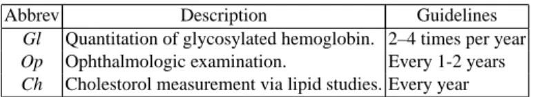
Three monitoring medical tests for diabetes treatment are given in Table 1. These are essential for controlling the condition of diabetic patients.1 Glycated hemoglobin measurements (Gl) provide information about the accumulated effect of glucose lev-els. Ophthalmologic examinations (Op) are important in the early identification and of complications related to eye sight. Cholesterol measurements via lipid studies (Ch) help identify possible complications relating to heart conditions.
Abbrev Description Guidelines
Gl Quantitation of glycosylated hemoglobin. 2–4 times per year
Op Ophthalmologic examination. Every 1-2 years
Ch Cholestorol measurement via lipid studies. Every year
Table 1. Types of services received by Patients and indicative guidelines.
4.1 Experimental Results
The data used in this paper was extracted from the Medicare transactional database.2 We used a subset of the de-identified data based on Medicare transactions from Western Australia (WA) for the period 1994 to 1998 inclusive. The sample data includes 4916 elderly diabetic patients. We have only limited demographic information about each patient, such as age, gender and location. For each patient we also have the sequence of diabetes-related monitoring tests they have received over the time interval. We identified clusters in which patterns associated with nine states for diabetes patients were found.
We study each of the three tests separately to find out how a patient’s treatment follows the guidelines. We also study the overall patterns which take all three tests into consideration. To this end we summarise all the events (the tests performed) into eight distinct types of events which are listed in Table 2. A sample patient record is illustrated in Figure 2. For example, the patient has taken test 6 (i.e., Op and Ch) in early 1994, followed by a test 5 (i.e., Gl and Ch) and so on.
Through this experiment we are interested in investigating the following issues which are of interest to medical experts with particular interest in changes to patterns of care in the management of Diabetes over time:
1
The Health Insurance Commission of Australiahttp://www.hic.gov.au.
2
All experiments were done on a Unix system and under Windows NT with the prototype writ-ten in Awk and MATLAB.
Test group Description Test group Description test 0 No test test 4 Gl and Op test 1 Gl only test 5 Gl and Ch test 2 Op only test 6 Op and Ch test 3 Ch only test 7 Gl, Op and Ch
Table 2. Eight possible test combinations tests for patients
1994 1995 1996 1997 1998 test6 * test5 * test5 * test3 * test1 * test5
test1 test1 test1test3 * test3 *test2 * test1 * test1* * * test5* test6 * test5 * * test1* * *
Fig. 2. A sample patient’s health record, showing the seven types of tests received over five years.
– Does there exist any temporal patternPtfor all patients who have one, two, or three
tests regularly?
– What features are there for those temporal patterns? and
– Does there exist any temporal subpattern inPtor between patternsPt’s?
Modelling DTS We assume that for each successive pair of time points in a DTS we
haveti+1 -ti = c (a unit constant). For mining temporal patterns from a real-world
dataset we use time gap as the time variable between events (e.g., the same test group) instead of natural time (e.g., day) between different events. For example, a patient record is given in Table 3.
Test group The day of test group taken Time gap between the same test group
1 1 time gap = 1 1 191 time gap = 190 2 331 time gap = 1 7 487 time gap = 1 2 779 time gap = 448 1 894 time gap = 703 6 947 time gap = 1
Table 3. A patient test group transactional record with time gap.
From Table 3 we apply pattern searching on state-space and use time gap as variable for each test group for structural pattern searching. This means that we may view the structural base as a set of vector sequence: S9×m ={S1,· · ·,Sm}, where each Si =
assigned to a prespecified group. Then the problem of structural pattern discovery for the sequence and its each subsequence Sij ={si1, si2,· · ·, sij : 1≤i≤9,1≤j ≤
m}of S on finite-state space can be formulated as a Haar’s function with Mahalanobis distance model.
Then we may also view the value-point process data asN-dimensional data set3:
V={V1,· · ·,Vm}, where each Vi= (v1i, v2i,· · ·, vNi)T, where theNis dependent
on how many statistical values relate to the structural base pattern searching. Then the problem of value-point pattern discovery can be formulated as stochastic distribution of the sequence and its subsequences Vj ={v1j, v2j,· · ·, vNj}of a discrete-valued time
series4.
On structural pattern searching We are investigating the data structural base to test
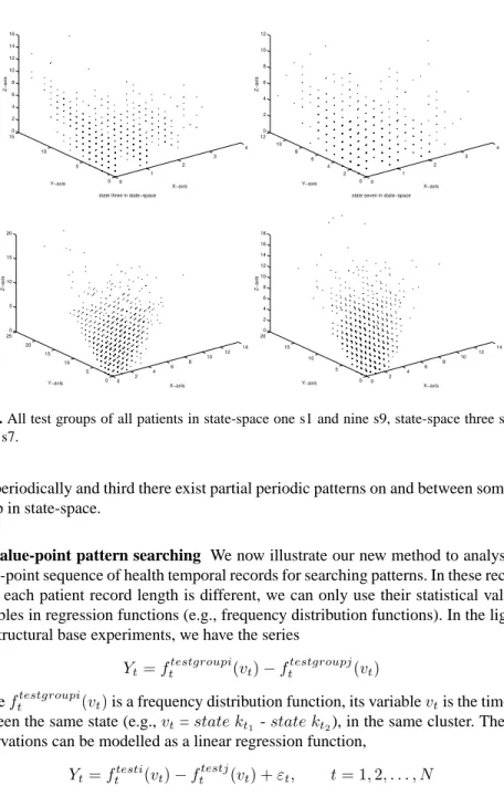
naturalness of the similarity and periodicity on Structural Base distribution. We consider seven test groups in the state-space for structural distribution:S = {s1, s2, . . . , s9}. For finding all levels patterns(or clusters), we applied Haar’s function (Equation 1) and distance function (Equation 4) on three-dimensional dataset for structural based pattern researching in state-space. First dimension is the test group, second dimension is the time gap between each test group and the third dimension is the time gap within the same test group.
For example for test group one and test group nine, in Figure 4, the X-axis represents the distribution frequency of test groups (e.g., in first dimension), the Y-axis represents distribution of time gap frequency between test groups (e.g., in second dimension) and the Z-axis represents distribution of frequency of time gap between the same test groups in state-space (e.g., in third dimension). Now we interpret an important result from the structural pattern searching: There exist similar time gap frequency patterns between and/or within state one and state nine for all test groups, this means, for example, pattern of patients not taking any test is similar to the pattern of patients taking test group one and test group two with the time gap increasing (or, decreasing).
We found some other results such as (1) there exist similar time gap frequency patterns between and/or within state two and state six for all test groups: the meaning is that the patients have not been given good care by doctors according to the clinical guidelines and (2) there exist similar and periodic time gap frequency patterns between state three and state seven for all test groups: the reason for the pattern is that the patients have been given good care by doctors according to the clinical guidelines.
In Figure 5, the x-axis represents natural integer sequenceNand the y-axis rep-resents the time gap for each state. Figure 5 explains some important facts: first that there exists the same time gap statistical distribution (e.g., the same tangent curve dis-tribution) between the test group 1, test group 2, test group 3 and test group 5. It also explains visits to doctors are stationary in different time gaps for those four types of test groups. Second, there exists a hidden periodic distribution which corresponds to patterns on the same state with different distances, this means patients visit their
doc-3
According to their structural distribution model
4
In fact, many practical problems in temporal data mining related to statistical modelling are explained in the context of regression models.
0 1 2 3 4 0 5 10 150 2 4 6 8 10 12 14 16 X−axis state one in state−space
Y−axis Z−axis 0 1 2 3 4 0 2 4 6 8 10 120 2 4 6 8 10 12 X−axis state nine in state−space
Y−axis Z−axis 0 2 4 6 8 10 12 14 0 5 10 15 20 250 5 10 15 20 X−axis state three in state−space
Y−axis Z−axis 0 2 4 6 8 10 12 14 0 5 10 15 200 2 4 6 8 10 12 14 16 18 X−axis state seven in state−space
Y−axis
Z−axis
Fig. 3. All test groups of all patients in state-space one s1 and nine s9, state-space three s3 and
seven s7.
tors periodically and third there exist partial periodic patterns on and between some test group in state-space.
On value-point pattern searching We now illustrate our new method to analyse the
value-point sequence of health temporal records for searching patterns. In these records, since each patient record length is different, we can only use their statistical value as variables in regression functions (e.g., frequency distribution functions). In the light of our structural base experiments, we have the series
Yt=f
testgroupi
t (vt)−f
testgroupj
t (vt) (7)
wherefttestgroupi(vt)is a frequency distribution function, its variablevtis the time gap
between the same state (e.g.,vt=state kt1 -state kt2), in the same cluster. Then the
observations can be modelled as a linear regression function,
Yt=fttesti(vt)−fttestj(vt) +εt, t= 1,2, . . . , N (8)
and we also consider theε(t)as an auto-regressionAR(2)model
εt0 =aεt0−1+bεt0−2+et0 (9)
wherea,bare constants dependent on sample dataset, andet0 with a small variance
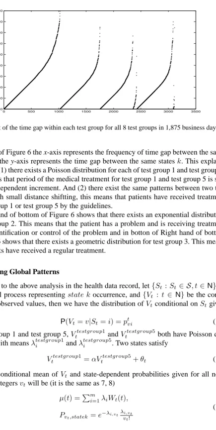
0 500 1000 1500 2000 2500 3000 3500 0 200 400 600 800 1000 1200 1400 1600 1800
Fig. 4. Plot of the time gap within each test group for all 8 test groups in 1,875 business days.
In top of Figure 6 the x-axis represents the frequency of time gap between the same states and the y-axis represents the time gap between the same statesk. This explains two facts: (1) there exists a Poisson distribution for each of test group 1 and test group 5. This means that period of the medical treatment for test group 1 and test group 5 is sta-tionary independent increment. And (2) there exist the same patterns between two test groups with small distance shiftting, this means that patients have received treatment for test group 1 or test group 5 by the guidelines.
Left hand of bottom of Figure 6 shows that there exists an exponential distribution for test group 2. This means that the patient has a problem and is receiving treatment for the identification or control of the problem and in botton of Right hand of bottom of Figure 6 shows that there exists a geometric distribution for test group 3. This means that patients have received a regular treatment.
4.2 Mining Global Patterns
According to the above analysis in the health data record, let{St:St∈ S, t∈N}be
a structural process representingstate k occurrence, and{Vt : t ∈ N}be the
corre-sponding observed values, then we have the distribution ofVtconditional onStgiven
by
P(Vt=v|St=i) =ptvi (10)
For test group 1 and test group 5,Vttestgroup1andVttestgroup5 both have Poisson dis-tribution with meansλtestgroupi 1andλtestgroupi 5. Two states satisfy
Vttestgroup1=αVttestgroup5+θt (11)
Then the conditional mean of Vt and state-dependent probabilities given for all
non-negative integersvtwill be (it is the same as 7, 8)
µ(t) =Pm i=1λiWt(t), Pvt,statek=e −λi,vtλi,vt vt! (12)
0 200 400 600 800 1000 1200 0 200 400 600 800 1000 1200 1400 1600 1800
frq for between t1 time distance
0 50 100 150 200 250 300 350 400 450 500 0 200 400 600 800 1000 1200 1400 1600
frq. between t5 time distance
0 500 1000 1500 2000 2500 3000
0 500 1000 1500
frq. between t2 time distance
0 100 200 300 400 500 600 700 800 900 1000 0 200 400 600 800 1000 1200 1400
frq. between t3 time distance
Fig. 5. Top: Time distance frequency distribution of test group 1 and test group 5 are Poisson
distributions. Bottom: Time distance frequency distribution of test group 2 is an exponential dis-tribution (Left) and Time distance frequency disdis-tribution of test group 3 is a geometric disdis-tribution (Right).
For test group 2,Vttestgroup2is an exponential distribution with parametersλtestgroupi 2
andµtestgroupi 2. Then the conditional exponential distribution ofVttestgroup2and state-dependent probabilities given for all non-negative integersvtwill be
µ(t) =Pm i=1λiWt(t), Pvt,test2= λ(i,vt)e (−λ(i,vt)(vt−µ)) v t> µ 0 vt< µ (13)
For test group 3,Vttestgroup3is a geometric distribution with parameterptestgroupi 3. Then the conditional geometric distribution ofVttestgroup3and state-dependent proba-bilities given for all non-negative integersvtwill be
µ(t) =Pm i=1λiWt(t), Pvt,testgroup3=p statek i,vt (1−p statek i,vt ) (vt−1) (14)
Test group 4, test group 6 and test group 7 are indepentent states. We use Haar func-tion and local polynomial funcfunc-tion for each of them to find their condifunc-tional distribufunc-tion
functionftestgroupk(t). We found that there exist some similar patterns between each
of their state but no patterns exist between each of their clusters of time gap, this means the patients have received number of treatments from test groupk(k= 4, 6, 7) similar but for different time periods.
The main results from structural pattern seaching and value-point pattern searching are:
– The behaviour of visiting doctors for pattients with just a diabetic is a Poisson
distribution, the meaning is that number of doctor visits by diabetic group people in the same of period(e.g., within 7 days) have the same distribution.
– The distribution of visiting pattern(taking tests) between the patient that has taken
more care and less care is log-normal distribution, the meaning is that the num-ber of doctor visits is not symmetric around the mean, but much extending to the right(e.g., pattern of less care)
– The other main combined-results on the health dataset are as follows:
1. There does exist some full periodic pattern within and between state 1 and state 5, this means the time gap between patients taking test 1, and time gap between patients taking test 1 & test 3 are both stationary.
2. There exist some partial periodic patterns between state 1, state 2, state 3 and state 5, this means the patients have sub-common problem such as they all have eye problem( e.g., taking more eye test, etc.).
3. There also exist some similar patterns between state 1, state 2, state 3 and state 5. This means there exists similar patterns of behaviour for patients visiting their doctors but for different tests.
In [2] three alternative feature vectors for representing variable-length patient health records were used. An interesting observation from there is that the average, residual, and deviance clusters have similar mean average and deviance values, but differ in their residual value. This shows the value of using the residual feature to identify intensive patterns of care during a relatively short time interval. In our approach, using a tempo-ral data mining method, we can find results (e.g., interesting patterns and unexpected patterns).
5
Concluding Remarks
This paper has presented a new approach based on hybrid models to form new models of application of data mining. The rough decision for pattern discovery comes from the structural level that is a collection of certain predefined similar patterns. The clusters of similar patterns are computed in this level by the choice of certain distance mea-sures. The point-value patterns are decided in the second level and the similarity and periodicity of a DTS are extracted. In the final level, we combine structural and value-point pattern searching into the wavelet’s feature-based regression models (WFMs) to obtain a global pattern picture and understand the patterns in a dataset better. Another approach to find similar and periodic patterns has been reported in [10, 11, 13, 12]; there the models used are based on hidden functional analysis. However, we have found that using different models at different levels produces better results.
The method guarantees finding different patterns if they exist with structural and valued probability distribution of a real-dataset. The results of preliminary experiments are promising.
References
1. R Agrawal, G Psaila, E L Wimmers, and M Zait. Querying shapes of histories. In
Proceed-ings of the 21st VLDB Conference, 1995.
2. R A Baxter, G J Williams, and H He. Feature selection for temporal health records. In
Proceedings of the 5th Pacific-Asia Conference on Knowledge Discovery and Data Mining,
2001.
3. C Bettini. Mining temportal relationships with multiple granularities in time sequences.
IEEE Transactions on Data & Knowledge Engineering, 1998.
4. G Das, K Lin, H Mannila, G Renganathan, and P Smyth. Rule discovery from time series. In Proceedings of the international conference on KDD and Data Mining(KDD-98), 1998. 5. G Das, D Gunopulos, and H Mannila. Finding similar time seies. In Principles of Knowledge
Discovery and Data Mining ’97, 1997.
6. A Haar. Zur theore der orthoganalen funktionen systeme. Annals of Mathematics 69:
331-371.
7. J Elder IV and D Pregibon. A statistical perspective on knowledge discovery in databases. In U Fayyad, G Piatetsky-Shapiro, P Smyth, and R Uthurusamy, editors, Advances in
Knowl-edge Discovery and Data Mining, pages 83–115. The MIT Press, 1995.
8. J B MacQueen. Some methods for classification and analysis of multivariate observations. In
5th Berkeley Symposium on Mathematical Statistics and Probability, pages 281–297, 1967.
9. C Li and G Biswas. Temporal pattern generation using hidden markov model based unsu-perised classifcation. In Proc. of IDA-99, pages 245–256, 1999.
10. W Q Lin and M A Orgun. Applied hidden periodicity analysis for mining discrete-valued time series. In Proceedings of ISLIP-99, pages 56–68, Demokritos Institute, Athens, Greece, 1999.
11. W Q Lin and M A Orgun. Temporal data mining using hidden periodicity analysis. In
Proceedings of ISMIS2000, University of North Carolina, USA, 2000.
12. W Q Lin, M A Orgun, and G J Williams. Temporal data mining using hidden markov-local polynomial models. In Proceedings of PAKDD2001, The University of Hongkong, Hong Kong, 2000.
13. W Q Lin, M A Orgun, and G J Williams. Temporal data mining using multilevel-local polynomial models. In Proceedings of IDEAL2000, The Chinese University of Hongkong, Hong Kong, 2000.
14. S Jajodia, S Sripada, and O Etzion, editors. Temporal databases: Research and Practice. Springer-Verlag, Lecture Notes in Computer Science, Volume 1399, 1998.
15. H L Resnikoff and R O Wells, editors. Wavelet Analysis, The scalable structure of
informa-tion. Springer-Verlag, 1998.
16. Z Huang. Clustering large data set with mixed numeric and categorical values. In