Statistical inference for varying coefficient models

(1)

STATISTICAL INFERENCE FOR VARYING COEFFICIENT MODELS

by

YIXIN CHEN

B.S., Henan University, China, 2008

M.S., Pittsburg State University, USA, 2010

AN ABSTRACT OF A DISSERTATION

submitted in partial fulfillment of the

requirements for the degree

DOCTOR OF PHILOSOPHY

Department of Statistics

College of Arts and Sciences

KANSAS STATE UNIVERSITY

Manhattan, Kansas

(2)

Abstract

This dissertation contains two projects that are related to varying coefficient models. The traditional least squares based kernel estimates of the varying coefficient model will lose some efficiency when the error distribution is not normal. In the first project, we pro-pose a novel adaptive estimation method that can adapt to different error distributions and provide an efficient EM algorithm to implement the proposed estimation. The asymptotic properties of the resulting estimator is established. Both simulation studies and real data examples are used to illustrate the finite sample performance of the new estimation proce-dure. The numerical results show that the gain of the adaptive procedure over the least squares estimation can be quite substantial for non-Gaussian errors.

In the second project, we propose a unified inference for sparse and dense longitudinal data in time-varying coefficient models. The time-varying coefficient model is a special case of the varying coefficient model and is very useful in longitudinal/panel data analysis. A mixed-effects time-varying coefficient model is considered to account for the within sub-ject correlation for longitudinal data. We show that when the kernel smoothing method is used to estimate the smooth functions in the time-varying coefficient model for sparse or dense longitudinal data, the asymptotic results of these two situations are essentially different. Therefore, a subjective choice between the sparse and dense cases may lead to wrong conclusions for statistical inference. In order to solve this problem, we establish a unified self-normalized central limit theorem, based on which a unified inference is proposed without deciding whether the data are sparse or dense. The effectiveness of the proposed unified inference is demonstrated through a simulation study and a real data application.

(3)

Key words: Varying coefficient models; adaptive estimation; local maximum likelihood; kernel smoothing; EM algorithm; dense longitudinal data; sparse longitudinal data; time-varying coefficient models; self-normalization.

(4)

STATISTICAL INFERENCE FOR VARYING COEFFICIENT MODELS

by

Yixin Chen

B.S., Henan University, China, 2008

M.S., Pittsburg State University, USA, 2010

A DISSERTATION

submitted in partial fulfillment of the

requirements for the degree

DOCTOR OF PHILOSOPHY

Department of Statistics

College of Arts and Sciences

KANSAS STATE UNIVERSITY

Manhattan, Kansas

2014

Approved by:

Major Professor Dr. Weixin Yao

(5)

Copyright

Yixin Chen

(6)

Abstract

This dissertation contains two projects that are related to varying coefficient models. The traditional least squares based kernel estimates of the varying coefficient model will lose some efficiency when the error distribution is not normal. In the first project, we pro-pose a novel adaptive estimation method that can adapt to different error distributions and provide an efficient EM algorithm to implement the proposed estimation. The asymptotic properties of the resulting estimator is established. Both simulation studies and real data examples are used to illustrate the finite sample performance of the new estimation proce-dure. The numerical results show that the gain of the adaptive procedure over the least squares estimation can be quite substantial for non-Gaussian errors.

In the second project, we propose a unified inference for sparse and dense longitudinal data in time-varying coefficient models. The time-varying coefficient model is a special case of the varying coefficient model and is very useful in longitudinal/panel data analysis. A mixed-effects time-varying coefficient model is considered to account for the within sub-ject correlation for longitudinal data. We show that when the kernel smoothing method is used to estimate the smooth functions in the time-varying coefficient model for sparse or dense longitudinal data, the asymptotic results of these two situations are essentially different. Therefore, a subjective choice between the sparse and dense cases may lead to wrong conclusions for statistical inference. In order to solve this problem, we establish a unified self-normalized central limit theorem, based on which a unified inference is proposed without deciding whether the data are sparse or dense. The effectiveness of the proposed unified inference is demonstrated through a simulation study and a real data application.

(7)

Key words: Varying coefficient models; adaptive estimation; local maximum likelihood; kernel smoothing; EM algorithm; dense longitudinal data; sparse longitudinal data; time-varying coefficient models; self-normalization.

(8)

List of Figures

1.1 Estimated coefficient functions with 95% pointwise confidence intervals (blue dot-ted line for Adapt and red solid line for LS) for model 1. . . 10 1.2 Estimated coefficient functions with 95% pointwise confidence intervals (blue

dot-ted line for Adapt and red solid line for LS) for model 2. . . 10 1.3 Estimated coefficient functions (solid curves) with 95% pointwise confidence

inter-vals (dotted curves) for Hong Kong environmental data. . . 12 1.4 Estimated coefficient functions (solid curves) with 95% pointwise confidence

inter-vals (dotted curves) for Boston housing data. . . 13 1.5 Residual QQ-plot for two data examples: (a) Hong Kong environmental data; (b)

Boston housing data. . . 14

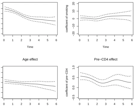
2.1 Application to AIDS data. Estimated coefficient curves for the baseline CD4 per-centage and the effects of smoking, age and pre-infection CD4 perper-centage on the percentage of CD4 cells. Solid curves, estimated effects; dashed curves, 95% self-normalization based confidence intervals; dotted curves, 95% bootstrap confidence intervals. . . 43

(11)

List of Tables

1.1 Model 1 estimation accuracy comparison–RASE and its standard error in brackets. . . 9 1.2 Model 2 estimation accuracy comparison–RASE and its standard error in

brackets. . . 9

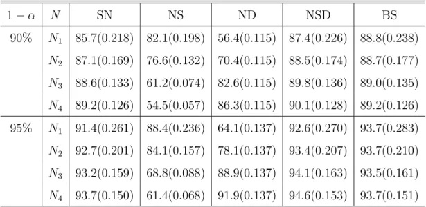
2.1 Average empirical coverage percentages and lengths, in brackets, for β0(t) of five confidence intervals. . . 39 2.2 Average empirical coverage percentages and lengths, in brackets, for β1(t) of

five confidence intervals. . . 40 2.3 Average empirical coverage percentages and lengths, in brackets, for β2(t) of

(12)

Acknowledgments

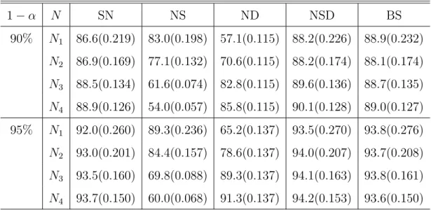
First and foremost, I would like to express my appreciation to my major professor, Dr. Weixin Yao, for all his encouragement, guidance and suggestions.

I would also like to thank Dr. Gary Gadbury, Dr. Juan Du and Dr. Xinming Ou for their willingness to serve on my committee and for their valuable insight.

In addition, I would like to thank Dr. Marianne Korten for her willingness to be the chairperson of the examining committee for my doctoral degree.

My gratefulness extends to everyone who supported me in any respect during the com-pletion of this dissertation.

(13)

Chapter 1 Adaptive Estimation for Varying

Coefficient Models

1.1 Introduction

Since the introduction in Cleveland, et al. (1992) and Hastie and Tibshirani (1993), vary-ing coefficient models have gained considerable attention due to their flexibility and good interpretability. They are useful extensions of the classical linear models and have been widely used to explore the dynamic pattern in many scientific areas, such as finance, eco-nomics, epidemiology, ecology, etc. By allowing coefficients to vary over the so-called index variable, the modeling bias can be significantly reduced and the ‘curse of dimensionality’ can be avoided (Fan and Zhang, 2008). In recent years, varying coefficient models have experienced rapid developments in both theory and methodology, see, for example, Wu, et al. (1998), Hoover, et al. (1998), Fan and Zhang (1999, 2000), Cai, et al. (2000), Fan and Huang (2005),Wang, et al. (2009),Wang and Xia (2009), etc. We refer readers toFan and Zhang (2008) for a nice and comprehensive survey.

Lety ∈ R1 _{be the response,} _x_{= (}_{x1, . . . , x}

(14)

is the index variable. The varying coefficient model is defined as y= d X j=1 gj(u)xj +, (1.1)

where{g1(u), . . . , gd(u)}T are unknown smooth coefficient functions. Throughout this

chap-ter, we assume the random error to be independent of (u, x), with mean 0 and a finite second-order moment σ2_{. By setting} _x

1 ≡1, it allows a varying intercept in the model.

Hastie and Tibshirani (1993), Hoover, et al. (1998),Chiang, et al. (2001), and Eubank, et al. (2004) proposed using smoothing spline to estimate coefficient functions. Polynomial spline was used in Huang, et al. (2002, 2004) and Huang and Shen (2004). Wu, et al.

(1998), Hoover, et al. (1998), Fan and Zhang (1999), and Kauermann and Tutz (1999) adopted kernel smoothing to estimate coefficient functions. Fan and Zhang (2000) further studied a two-step estimation procedure to deal with the situation where the coefficient functions admit different degrees of smoothness. Recently, Wang and Xia (2009) proposed a shrinkage estimation procedure to select important nonparametric components. Wang, et al. (2009) developed a highly robust and efficient procedure based on local ranks.

Nevertheless, most of existing methods used least squares type criteria in estimation, which corresponds to the local likelihood when the error is normal. However, in the absence of normality, the traditional least squares based estimators will lose some efficiency. In this chapter, we propose a novel adaptive kernel estimation procedure for varying coefficient models. The new adaptive method combines the kernel density estimation and the local maximum likelihood estimation such that the new estimator can adapt to different error distributions. The new adaptive estimator is shown to enjoy the asymptotic oracle property, i.e., it is asymptotically as efficient as if the error density were known. An efficient EM algorithm is proposed to implement the adaptive estimation method. We demonstrate through a simulation study that the new estimate is more efficient than the existing least squares based kernel estimate when the error distribution deviates from normal. In addition,

(15)

when the error is exactly normal, the new method is broadly comparable to the existing kernel approach. We further illustrate the effectiveness of the proposed adaptive estimation method with two real data examples.

The rest of this chapter is organized as follows. In Section 1.2, we introduce the new adaptive estimation method for the varying coefficient models and the EM algorithm. In Section 1.3, we compare our proposed adaptive estimation with the traditional least squares based estimation for five different error densities through a simulation study and then apply the new method to two real data examples. We conclude this chapter with a brief discussion in Section 1.4. All technical conditions and proofs are relegated to Section 1.5.

1.2 New Adaptive Estimation

1.2.1 Introduction to The New Method

Suppose that {xi, ui, yi, i = 1, . . . , n} is a random sample from model (1.1). For u in a

neighborhood of u0, we can approximate varying coefficient functions locally as

gj(u)≈gj(u0) +g0j(u0)(u−u0)≡bj +cj(u−u0), for j = 1, . . . , d. (1.2)

The traditional local linear estimation of (1.1) is to minimize

n X i=1 Kh(ui−u0) " yi− d X j=1 {bj +cj(ui −u0)}xij #2 , (1.3)

for a given kernel density K(·) and a bandwidth h, where Kh(t) = h−1K(t/h). It is well

known that the choice of kernel function is not critical in terms of estimation efficiency. Throughout this chapter, a Gaussian kernel will be used for K(·). Due to the least squares in (1.3), the resulting estimate may lose some efficiency when the error distribution is not normal. Therefore, it is desirable to develop an estimation procedure which can adapt to

(16)

different error distributions.

Letf() be the density function of . Iff() were known, it would be natural to estimate the local parameters in (1.2) by maximizing the following local log-likelihood function

n X i=1 Kh(ui−u0) logf " yi− d X j=1 {bj +cj(ui−u0)}xij # . (1.4)

However, in practice, f() is generally unknown but can be replaced by a kernel density estimate based on the initial estimated residual ˜1, . . . ,˜n

˜ f(i) = 1 n n X j6=i Kh0(i−˜j), for i, j = 1,2, ..., n (1.5) where ˜i = yi − Pd

j=1˜gj(ui)xij and ˜gj(·) can be estimated by least squares (or L1 norm, i.e., median regression) based local linear estimate (1.3). Here we use leave-one-out kernel density estimate for f(i) to remove the estimation bias. Let θ = (b1, . . . , bd, c1, . . . , cd)T.

Then our proposed adaptive local linear estimate for the local parameter θ is

ˆ θ= arg max θ Q(θ), (1.6) where Q(θ) = n X i=1 Kh(ui−u0) log 1 n X j6=i Kh0 " yi− d X l=1 {bl+cl(ui−u0)}xil−˜j #! . (1.7)

The idea of adaptiveness can be traced back to Beran (1974) and Stone (1975), where the adaptive estimation was proposed for location models. Later, this idea was extended to regression, time series and other models, see Bickel (1982), Manski (1984), Steigerwald

(1992), Schick (1993), Drost and Klaassen (1997), Hodgson (1998), Yuan and De Gooijer

(2007), andYuan(2009). Linton and Xiao(2007) proposed an elegant adaptive nonparamet-ric regression estimator by maximizing the local likelihood function. In fact, the adaptive

(17)

method proposed in Linton and Xiao (2007) can be seen as a special case of ours when d= 1 in (1.1). Wang and Yao(2012) extended the idea of adaptive estimation to sufficient dimension reduction.

1.2.2 Computation: An EM Algorithm

Unlike least squares criterion, (1.6) does not have an explicit solution. In this section, we propose an EM algorithm to maximize it by extending the generalized modal EM algorithm proposed in Yao (2013).

Let θ(0) be an initial parameter estimate, such as the least squares (or L1 norm, i.e., median regression) based local linear estimate. We can update the parameter estimate according to the following algorithm.

Algorithm 1.2.1. At (k+ 1)th step, we calculate the following E and M steps:

E-Step: Calculate the classification probabilities,

p(_ijk+1) = Kh0 h yi− Pd l=1{b (k) l +c (k) l (ui−u0)}xil−˜j i P j6=iKh0 h yi− Pd l=1{b (k) l +c (k) l (ui−u0)}xil−˜j i ∝Kh0 " yi− d X l=1 {b(_lk)+c(_lk)(ui−u0)}xil−˜j # , 1≤j 6=i≤n. (1.8) M-Step: Update θ(k+1), θ(k+1)= arg max θ n X i=1 X j6=i ( p(_ijk+1)Kh(ui−u0) log Kh0 " yi− d X l=1 {bl+cl(ui−u0)}xil−˜j #!) = arg min θ n X i=1 X j6=i n p(_ijk+1)Kh(ui−u0) yi−˜j −zTi θ 2o , = n X i=1 X j6=i p(_ijk+1)Kh(ui−u0)zizTi !−1 _n X i=1 X j6=i p(_ijk+1)Kh(ui−u0)(yi−˜j)zi (1.9)

(18)

where zi = {xTi ,xTi (ui−u0)}T and the second equation follows the use of Gaussian

kernel for density estimation.

The above EM algorithm monotonically increases the estimated local log-likelihood (1.7) after each iteration, as shown in the following theorem.

Theorem 1.2.1. Each iteration of the above E and M steps will monotonically

in-crease the local log-likelihood (1.7), i.e.,

Q(θ(k+1))_>Q(θ(k)),

for all k, where Q(·) is defined as in (1.7).

1.2.3 Asymptotic Result

We now derive the asymptotic distribution of the proposed adaptive local linear estimator of θ. Define µk = R uk_K₍_u_)d_u _and _ν k = R uk_K2₍_u_)d_u_{. Let} _H _{= diag(1}_{, h}₎_⊗_I d with ⊗

denoting the Kronecker product and Idbeing the d×didentity matrix. Let q(·) denote the

marginal density of u, and

Γjk(ui) = E(xijxik|ui) for 1≤j, k ≤d, i= 1, ..., n, (1.10)

Γ(u0) = {Γjk(u0)}₁₆_j,k₆_d. (1.11)

Theorem 1.2.2. Suppose that the regularity conditions in Section 1.5 hold. Then, with probability approaching 1, there exists a consistent local maximizer

ˆ θ = (ˆb1, . . . ,ˆbd,cˆ1, . . . ,ˆcd)T of (1.7) such that √ nh ( H(ˆθ−θ)−S−1h 2 2 d X j=1 g00_j(u0)ψj(1 +op(1)) ) D →N(02d, δ1−2δ2q(u0)−1S−1ΛS−1),

(19)

where02dis a2d×1vector with each entry being 0,ρ(·) = logf(·), δ1 =E ρ00(i) , δ2 = Eρ0(i)2 , S =    1 0 0 µ2    ⊗ Γ(u0), Λ =    ν0 ν1 ν1 ν2    ⊗ Γ(u0), ψj =    µ2 µ3    ⊗ (Γjk(u0)) T 1≤k≤d, and Γ(u0) is given by (1.11).

A sketch of the proof of the above theorem is provided in Section 1.5. As shown in

Linton and Xiao (2007), one important property of the proposed adaptive estimate is its asymptotic oracle property, i.e., it achieves the same asymptotic efficiency as if the error density were known. Therefore, the effect of estimating f by kernel density estimate will not affect the asymptotic distribution of the resulting estimator of θ.

1.3 Examples

1.3.1 Simulation Study

In this section, we conduct a simulation study to compare the proposed adaptive estimation (Adapt) with the traditional least squares based kernel estimation (LS) for varying coeffi-cient models. The following five error distributions of were considered in our numerical experiment: 1. N(0,1); 2. t3; 3. 0.5N(−1,0.52_{) + 0}_.₅_N₍₁_,₀_.₅2_); 4. 0.3N(−1.4,1) + 0.7N(0.6,0.42); 5. 0.9N(0,1) + 0.1N(0,102_).

The standard normal distribution serves as a baseline in our comparison. The second one is a t-distribution with 3 degrees of freedom. The third density is bimodal and the fourth

(20)

one is left skewed. The last one is a contaminated normal mixture distribution, where 10% of the data from N(0,102_{) are most likely to be outliers.}

For each of the above error distributions, we consider the following two models:

Model 1: y=g1(u) +g2(u)x1+g3(u)x2+,where g1(u) = exp(2u−1), g2(u) = 8u(1−u), and g3(u) = 2 sin2(2πu).

Model 2: y=g1(u) +g2(u)x1+g3(u)x2+,whereg1(u) = sin(2πu), g2(u) = (2u−1)2+ 0.5, and g3(u) = exp(2u−1)−1.

In both models, x1 and x2 follow a standard normal distribution with correlation coefficient γ = 1/√2. The index variable uis a uniform random variable on [0, 1], and is independent of (x1, x2). We conduct two simulations with sample sizen=200 and 400 respectively, each with 200 data replications. There are two bandwidths in the estimation, h in the local log-likelihood and h0 in the kernel density estimation. The bandwidthh is chosen by cross-validation with more details in Fan and Zhang (1999), and h0 =h/log(n) following Linton

and Xiao (2007). The performance of estimator ˆg(·) is assessed via the square root of the average squared errors (RASE; Cai, et al., 2000; Wang, et al.,2009),

RASE2 = 1 N N X k=1 3 X j=1 [ˆgj(uk)−gj(uk)]2, (1.12)

whereuk, k= 1, . . . , N,are the equally spaced grid points at which the functionsgj(·) were

evaluated. We used N=200 in the numerical studies.

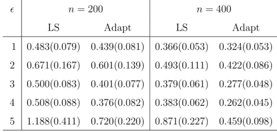
The simulation results are summarized in Tables 1.1 and 1.2. We can clearly see that the proposed adaptive estimation outperforms the least squares method when the error is non-normal. The gain in estimation efficiency can be quite substantial even for moderate sample sizes. When the error follows exactly normal distribution, our approach is still broadly comparable with the least squares based method.

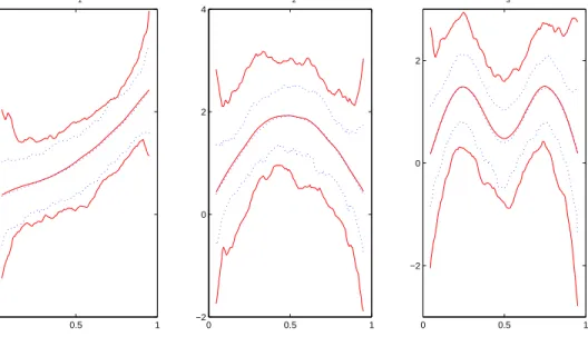
Figures 1.1 and 1.2 plot the estimated coefficient functions and the 95% pointwise con-fidence intervals based on a typical sample when n=200 and the error distribution is the

(21)

contaminated normal mixture (Case 5). It is clear that the adaptive estimation method provides narrower confidence intervals than the least squares based method, as expected.

Table 1.1: Model 1 estimation accuracy comparison–RASE and its standard error in brack-ets. n = 200 n= 400 LS Adapt LS Adapt 1 0.483(0.079) 0.439(0.081) 0.366(0.053) 0.324(0.053) 2 0.671(0.167) 0.601(0.139) 0.493(0.111) 0.422(0.086) 3 0.500(0.083) 0.401(0.077) 0.379(0.061) 0.277(0.048) 4 0.508(0.088) 0.376(0.082) 0.383(0.062) 0.262(0.045) 5 1.188(0.411) 0.720(0.220) 0.871(0.227) 0.459(0.098)

Table 1.2: Model 2 estimation accuracy comparison–RASE and its standard error in brack-ets. n = 200 n= 400 LS Adapt LS Adapt 1 0.362(0.077) 0.380(0.074) 0.263(0.051) 0.275(0.049) 2 0.618(0.301) 0.566(0.201) 0.431(0.129) 0.384(0.076) 3 0.412(0.091) 0.351(0.080) 0.290(0.059) 0.215(0.041) 4 0.407(0.102) 0.319(0.089) 0.291(0.061) 0.207(0.051) 5 1.133(0.397) 0.669(0.224) 0.828(0.224) 0.436(0.101)

1.3.2 Real-Data Applications

Example 1 (Hong Kong environmental data). We now illustrate the adaptive estimation

method via an application to an environmental data set. The data were collected daily in Hong Kong from January 1, 1994, to December 31, 1995 and have been analyzed byFan and Zhang (1999),Cai, et al. (2000),Xia, et al. (2002) and Fan and Zhang(2008). In this data

(22)

0 0.5 1 −2 0 2 4 (a) g₁(u) 0 0.5 1 −2 0 2 4 (b) g₂(u) 0 0.5 1 −2 0 2 (c) g₃(u)

Figure 1.1: Estimated coefficient functions with 95% pointwise confidence intervals (blue dotted line for Adapt and red solid line for LS) for model 1.

0 0.5 1 −2 0 2 (a) g 1(u) 0 0.5 1 0 2 4 (b) g 2(u) 0 0.5 1 −2 0 2 4 (c) g 3(u)

Figure 1.2: Estimated coefficient functions with 95% pointwise confidence intervals (blue dotted line for Adapt and red solid line for LS) for model 2.

set, a collection of daily measurements of pollutants and other environmental factors are included. Following Fan and Zhang (1999), we consider three pollutants: sulphur dioxide

(23)

x2 (in µg/m3), nitrogen dioxidex3 (inµg/m3), and respirable suspended particulatesx4 (in µg/m3_{) (this variable is named as ‘dust’ in} _{Fan and Zhang} ₍₁₉₉₉_), _{Fan and Zhang} ₍₂₀₀₈_), and Cai, et al. (2000)). The response variable is the logarithm of the number of daily hospital admissions y. We setx1 = 1 as the intercept term and let u denote time which is scaled to the interval [0, 1]. As in the previous analyses, all three predictors are centered. The following varying coefficient model is considered to investigate the relationship between y and the levels of pollutants x2,x3, and x4.

y =g1(u) +g2(u)x2+g3(u)x3+g4(u)x4+.

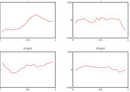
We set aside 50 observations as testing set. The bandwidth h, selected by leave-one-out cross-validation, is around 0.146. The estimated coefficient functions together with 95% pointwise confidence intervals are depicted in Figure 1.3. We also compare the median squared prediction errors, MSPE = Median{(yj −yˆj)2, j = 1, . . . , k}, from our adaptive

approach and the traditional least squares estimation, where k = 50 and ˆyj = ˆg1(uj) +

ˆ

g2(uj)xj2+ˆg3(uj)xj3+ˆg4(uj)xj4. The MSPE from our adaptive approach is 0.0183, compared to 0.0178 from the LS estimation.

In Figure1.5(a), we give the residual QQ-plot for Hong Kong environmental data. From the plot, we can see that the residual is very close to normal, which explains why the MSPE of the adaptive approach is close to the MSPE of the LS estimation.

Example 2 (Boston housing data). The Boston Housing Data (corrected version (Gilley

and Pace, 1996)), which has been analyzed by Fan and Huang (2005) and Wang and Xia

(2009), is publicly available in the R package mlbench, (http://cran.r-project.org/). In this data set, the median value of owner-occupied homes in 506 U.S. census tracts in the Boston area in 1970 and some variables that might explain the variation of housing value are included. FollowingFan and Huang (2005) andWang and Xia(2009), we consider seven in-dependent variables: CRIM (per capita crime rate by town), RM (average number of rooms per dwelling), TAX (full-value property-tax rate per $10,000), NOX (nitric oxides

(24)

concen-0 0.5 1 5.2 5.6 6 (a) g1(u) 0 0.5 1 −0.01 0 0.01 (b) g₂(u) 0 0.5 1 −0.01 0 0.01 (c) g₃(u) 0 0.5 1 −0.01 0 0.01 (d) g₄(u)

Figure 1.3: Estimated coefficient functions (solid curves) with 95% pointwise confidence intervals (dotted curves) for Hong Kong environmental data.

tration parts per 10 million), PTRATIO (pupil-teacher ratio by town), AGE (proportion of owner-occupied units built prior to 1940), and LSTAT (lower status of the population). The response variable is CMEDV (corrected median value of owner-occupied homes in USD 1000’s). We denote the covariates CRIM, RM, TAX, NOX, PTRATIO, and AGE to be x2, x3, . . . , x7, respectively. We take x1 = 1 as the intercept term and u =

√

LSTAT. By doing so, we can fit different regression models at different lower status population per-centage (Fan and Huang, 2005). Following Fan and Huang (2005) we use the square root transformation on the index variable LSTAT to make the data symmetrically distributed. We construct the following varying coefficient model

yi =g1(ui) +

7 X

j=2

gj(ui)xij +i.

Similar to the analysis in the previous example, we set aside 50 observations for checking prediction errors. The bandwidth h was selected by leave-one-out cross-validation, which is around 0.294. The estimated coefficient functions are depicted in Figure 1.4. From the

(25)

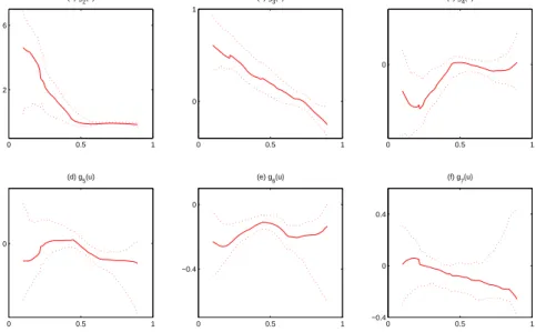
plot, we can see that the coefficient functions of x2 (CRIM) and x3 (RM) vary over time. The coefficient functions of x4 (TAX), x5 (NOX), and x7 (AGE) are very close to zero and the coefficient function of x6 (PTRATIO) shows no significant trend. These discoveries are consistent with those fromFan and Huang(2005) andWang and Xia(2009). In terms of the median squared prediction error (MSPE), the MSPE from our adaptive approach is 0.0484, compared to 0.0604 from the LS estimation.

In Figure 1.5 (b), we give the residual QQ-plot for Boston housing data. Based on the tails of the QQ-plot, there is a clear deviation of the residuals from normal, which explains why the MSPE of the adaptive approach is much smaller than the MSPE of the LS estimation. 0 0.5 1 2 6 (a) g 2(u) 0 0.5 1 0 1 (b) g 3(u) 0 0.5 1 0 (c) g 4(u) 0 0.5 1 0 (d) g 5(u) 0 0.5 1 −0.4 0 (e) g 6(u) 0 0.5 1 −0.4 0 0.4 (f) g 7(u)

Figure 1.4: Estimated coefficient functions (solid curves) with 95% pointwise confidence intervals (dotted curves) for Boston housing data.

1.4 Discussion

In this chapter, we proposed an adaptive estimation for varying coefficient models. The new estimation procedure can adapt to different errors and thus provide a more efficient

(26)

−4 −2 0 2 4 −0.4 −0.2 0 0.2 0.4

(a) Residual QQ−Plot of the Envionmental Data

−4 −2 0 2 4 −20 −10 0 10 20

(b) Residual QQ−Plot of the Boston Housing Data

Figure 1.5: Residual QQ-plot for two data examples: (a) Hong Kong environmental data; (b) Boston housing data.

estimate than the traditional least squares based estimate. Simulation studies and two real data applications confirmed our theoretical findings.

It will be interesting to know whether we can also perform some adaptive hypothesis tests for the coefficient functions using the estimated error density. For example, we might be interested in testing some parametric assumptions, such as constant or zero, for the coefficient functions. It requires more research about whether the Wilks phenomenon for generalized likelihood ratio statistic proposed byFan, et al.(2001) still holds for the proposed adaptive varying coefficient models.

The idea of the proposed adaptive estimator might also be generalized to many other models, such as varying coefficient partial linear models and nonparametric additive models. In addition, by combining this adaptive idea with shrinkage estimation, we can develop adaptive variable selection procedures. Such study is under way.

(27)

1.5 Proofs

We first impose some regularity conditions. Conditions:

1. K(·) is bounded, symmetric, and has bounded support and bounded derivative;

2. {xi}i,{ui}i,{i}i are independent and identically distributed and{i}i is independent

of {xi}i and {ui}i. Additionally, the predictor x has a bounded support;

3. The probability distribution function f(·) of has bounded continuous derivatives up to order 4. Let ρ() = logf(). Assume E[ρ0(i)] = 0, E[ρ

00

(i)]< ∞, E[ρ

0

(i)2]< ∞

and ρ000(·) is bounded;

4. The marginal density of u has a continuous second derivative in some neighborhood of u0 and q(u0)6= 0;

5. h→0, nh→ ∞ asn → ∞ and h0 =h/log(n);

6. gj(·) has bounded, continuous 3rd derivatives for 1≤j ≤d.

These conditions are adopted fromFan and Zhang(1999) andLinton and Xiao(2007). They are not the weakest possible conditions. For instance, the independence of {xi}i and {i}i

(28)

Proof of Theorem

1.2.1

Note that Q(θ(k+1))−Q(θ(k)) = n X i=1 Kh(ui−u0) log    P j6=iKh0 h yi−Pd_l₌₁ n b_l(k+1)+c_l(k+1)(ui−u0) o xil−˜j i P j6=iKh0 h yi − Pd l=1 n b_l(k)+c_l(k)(ui−u0) o xil−˜j i    = n X i=1 Kh(ui−u0) log X j6=i   Kh0 h yi− Pd l=1 n b_l(k)+c_l(k)(ui−u0) o xil−˜j i P j6=iKh0 h yi−Pd_l₌₁ n b_l(k)+c_l(k)(ui−u0) o xil−˜j i   ×   Kh0 h yi− Pd l=1 n b_l(k+1)+c_l(k+1)(ui−u0) o xil−˜j i Kh0 h yi− Pd l=1 n b_l(k)+c_l(k)(ui−u0) o xil−˜j i   = n X i=1 Kh(ui−u0) log    X j6=i p(_ijk+1) Kh0 h yi−Pd_l₌₁ n b_l(k+1)+c_l(k+1)(ui−u0) o xil−˜j i Kh0 h yi−Pd_l₌₁ n b_l(k)+c_l(k)(ui−u0) o xil−˜j i    , where p(_ijk+1) = Kh0 h yi− Pd l=1{b (k) l +c (k) l (ui−u0)}xil−˜j i P j6=iKh0 h yi−Pd_l₌₁{b (k) l +c (k) l (ui−u0)}xil−˜j i.

From the Jensen’s inequality, we have

Q(θ(k+1))−Q(θ(k)) > n X i=1 Kh(ui−u0) X j6=i p(_ijk+1)log    Kh0 h yi− Pd l=1 n b_l(k+1)+c_l(k+1)(ui−u0) o xil−˜j i Kh0 h yi−Pd_l₌₁ n b_l(k)+c_l(k)(ui−u0) o xil−˜j i    .

(29)

Proof of Theorem

1.2.2

Note that the estimator ˆθ is the maximizer of the following objective function

arg max θ n X i=1 Kh(ui −u0) log ˜f " yi− d X l=1 {bl+cl(ui−u0)}xil # , (1.13) where ˜ f(i) = 1 n X j6=i Kh0(i−˜j)

is the kernel density estimate of f(·), and ˜i is the residual based on the least squares local

linear estimate. By the adaptive nonparametric regression result ofLinton and Xiao(2007), the asymptotic result of ˆθ in (1.13) is the same whether the true densityf(·) is used or not. Therefore, we will mainly proof the existence and asymptotic distribution of ˆθ assuming f(·) is known.

We will first prove that with probability approaching 1, there exists a consistent local maximizer ˆθ= (ˆb1, . . . ,ˆbd,ˆc1, . . . ,ˆcd)T of (1.7) such that

H(ˆθ−θ) =Op{(nh)−1/2 +h2}.

Then we establish the asymptotic distributions for such consistent estimate.

Denote θ∗ = Hθ, x∗_i = (xi1, xi2, ..., xid,(ui−_hu0)xi1, ...,(ui−_hu0)xid)T, Ki = Kh(ui −u0), R(ui,xi) = Pd_j₌₁gj(ui)xij −Pd_j₌₁[bj +cj(ui −u0)]xij, and an = (nh)−1/2+h2. Let ρ(·) =

logf(·), we have the objective function

L(θ) = 1 n n X i=1 Kiρ(yi−θ∗Tx∗i) =L(θ ∗ ).

It is sufficient to show that for any given η >0, there exists a large constant csuch that

(30)

whereµhas the same dimension asθ,anis the convergence rate. By using Taylor expansion, it follows that L(θ∗+anµ)−L(θ∗) = 1 n n X i=1 Ki{ρ(i+R(ui,xi)−anµTx∗i)−ρ(i+R(ui,xi))} = −1 n n X i=1 Kiρ 0 (i+R(ui,xi))anµTx∗i + 1 2n n X i=1 Kiρ 00 (i+R(ui,xi))a2n(µ T_x∗ i) 2 − 1 6n n X i=1 Kiρ 000 (zi)a3n(µ T_x∗ i) 3 ∆ = I1+I2+I3,

whereziis a value betweeni+R(ui,xi)−anµTx∗i andi+R(ui,xi). ForI1 =−1_nPn_i₌₁Kiρ

0 (i+ R(ui,xi))anµTx∗i,E(I1) =−E Kiρ 0 (i+R(ui,xi))anµTx∗i

. By using Taylor expansion,

ρ0(i+R(ui,xi))≈ρ 0 (i) +ρ 00 (i)R(ui,xi) + 1 2ρ 000 (i)R2(ui,xi).

Based on the assumption that is independent of u and x, and E[ρ0(i)] = 0, we have

E(I1)≈ −anE Ki ρ00(i)R(ui,xi) + 1 2ρ 000 (i)R2(ui,xi) µTx∗_i . Since R(ui,xi) = Pd j=1gj(ui)xij− Pd j=1[bj +cj(ui−u0)]xij = d X j=1 [ ∞ X m=2 1 m!g (m) j (u0)(ui−u0)m]xij = Op(h2),

then 1₂ρ000(i)R2(ui,xi) = [Op(h2)]2 = Op(h4), which is a smaller order than ρ

00

(31)

Thus, E(I1)≈ −anE n Kiρ 00 (i)R(ui,xi)µTx∗i o =−anE h ρ00(i) i EKiR(ui,xi)µTx∗i . Since δ1 = E ρ00(i) , then E(I1)≈ −anδ1E KiR(ui,xi)µTx∗i =−anδ1E E R(ui,xi)µTx∗i|ui Ki . By µT_x∗ i ≤ kµk · kx ∗ ik=ckx ∗ ik, we have E(I1) = O(anch2). var(I1) = 1 nvar n Kiρ 0 (i+R(ui,xi))anµTx∗i o = 1 n{E(A 2₎₋_[E(_A_)]2_}_, where A=Kiρ 0 (i+R(ui,xi))anµTx∗i. Sinceδ2 = E ρ0(i)2 , then E(A2) = EnK_i2ρ0(i+R(ui,xi))2a2n(µ T_x∗ i) 2o ≈ a2_nEnK_i2ρ0(i)2(µTx∗i)2 o = a2_nδ2E E(µTx∗_i)2|ui Ki2 = O a2_nc21 h .

Note that [E(A)]2 = [O(anch2)]

2 E(A2), then var(I1) ≈ 1 nE(A 2_{) =} _{O a}2 nc2 1nh . Hence, I1 = E(I1) +Op( p var(I1)) =Op(anch2) +Op q a2 nc2 1nh =Op(ca2n). For I2 = 1 2n n X i=1 Kiρ 00 (i+R(ui,xi))a2n(µTx ∗ i)2,

(32)

we have E(I2) = 1 2a 2 nE n Kiρ 00 (i+R(ui,xi))(µTx∗i)2 o = 1 2a 2 nE n ρ00(i)Ki(µTx∗i)2 o (1 +o(1)) = 1 2a 2 nδ1E EµTx∗_ix_i∗Tµ|ui Ki (1 +o(1)) = 1 2a 2 nδ1µ T EEx∗_ix_i∗T|ui Ki µ(1 +o(1)). Note thatx∗_ix∗T i = xijxik ui−_hu0 l 1≤j,k≤d,l=0,1,2 and Γjk(ui) = E(xijxik|ui) for 1≤j, k ≤d, then E ( E ( xijxik ui−u0 h l |ui ) Ki ) = E ( E(xijxik|ui) ui−u0 h l Ki ) = E ( Γjk(ui) ui−u0 h l Ki ) .

By using Taylor expansion, we obtain

E ( E ( xijxik ui−u0 h l |ui ) Ki ) = 1 h Z Γjk(ui) ui−u0 h l K(ui−u0 h )q(ui)dui = q(u0)Γjk(u0) Z tlK(t)dt(1 +o(1)). So we have E(I2) = 1 2a 2 nδ1q(u0)µTSµ(1 +o(1)), where S=    1 0 0 µ2   ⊗Γ(u0) is a 2d×2d matrix. Thus, E(I2) =O(a2nδ1q(u0)µTSµ)

(33)

and var(I2) = a4 n 4nvar h ρ00(i+R(ui,xi))Ki(µTx∗i) 2i = a 4 n 4n E(B2)−[E(B)]2 , where B =ρ00(i+R(ui,xi))Ki(µTx∗i)2. Let δ3 = E ρ 00 (i)2 , then E(B2) = Enρ00(i+R(ui,xi))2Ki2(µTx ∗ i)4 o ≈ Enρ00(i)2Ki2(µ T x∗_i)4o = δ3EK_i2(µTx∗_i)4 = O 1 h .

Note that [E(B)]2 _{= [}_O_(1)]2 ₌ _O₍₁₎ _E(_B2_{), so var(}_I

2) = O

a4n

nh

. Based on the result I2 = E(I2) +Op(

p

var(I2)) and the assumptionnh→ ∞, it follows that

I2 =a2_nδ1q(u0)µTSµ(1 +op(1)). Similarly, I3 =−₆1_nPn_i₌₁Kiρ 000 (zi)a3n(µTx ∗ i)3 =Op(a3n).

Assume δ1 < 0. Noticing that S is a positive matrix, kµk = c, we can choose c large enough such that I2 dominates both I1 and I3 with probability at least 1−η. Thus P

supkµk=cL(θ∗+anµ)< L(θ∗) ≥1−η. Hence with probability approaching 1, there

ex-ists a local maximizer ˆθ∗ such that ˆ θ∗−θ∗ ≤anc, wherean= (nh) −1/2₊_h2_{. Based on the} definition ofθ∗, we can get, with probability approaching 1, H(ˆθ−θ) = Op((nh)−1/2+h2).

(34)

maximizes L(θ), then L0(ˆθ) = 0. By Taylor expansion, 0 = L0(ˆθ) =L0(θ0) +L 00 (θ0)(ˆθ−θ0) + 1 2L 000 (˜θ)(ˆθ−θ0)2,

where ˜θ is a value between ˆθ and θ0. Then ˆθ−θ0 =−[L

00 (θ0)]−1L 0 (θ0)(1 +op(1)). Since L(θ) = L(θ∗) = 1_nPn i=1Kiρ(yi −θ ∗T x∗_i) and yi −θ ∗T x∗_i = i +R(ui,xi), then L 00 (θ∗) = 1 n Pn i=1Kiρ 00

(i+R(ui,xi))x∗ix∗iT. We have the following expectation,

E[L00(θ∗)] = Enρ00(i +R(ui,xi))Kix∗ix ∗T i o ≈ Enρ00(i)Kix∗ix ∗T i o = δ1E Ex∗_ix∗_iT|ui Ki = δ1q(u0)S(1 +o(1)).

Throughout this chapter, we consider the element-wise variance of a matrix,

var[L00(θ∗)] = 1 nvar n Kiρ 00 (i+R(ui,xi))x∗ix ∗T i o =O 1 nh .

Based on the result L00(θ∗) = E[L00(θ∗)] +Op(

p

var[L00(θ∗)]) and the assumption nh→ ∞, it follows that

L00(θ∗) =δ1q(u0)S(1 +op(1)).

For L0(θ∗), we can divide it into two parts.

L0(θ∗) ≈ −1 n n X i=1 Kiρ 0 (i)x∗i − 1 n n X i=1 Kiρ 00 (i)R(ui,xi)x∗i ∆ = −wn−νn.

(35)

The asymptotic result is determined by wn. In order to find the order of νn, we compute

the following things.

E(νn) = E h Kiρ 00 (i)R(ui,xi)x∗i i =δ1E{E{R(ui,xi)x∗i|ui}Ki}.

Since g_j000(·) is bounded, then we have

R(ui,xi) = d X j=1 ( _∞ X m=2 1 m!g (m) j (u0)(ui −u0)m ) xij = d X j=1 1 2g 00 j(u0)(ui−u0)2xij(1 +op(1)). By x∗_i = (xi1, ..., xid,(ui−_hu0)xi1, ...,(ui−_hu0)xid)T, R(ui,xi)x∗i ≈   (ui−u0)2 2 ( _d X j=1 g_j00(u0)xij ) xik ! 1≤k≤d , (ui−u0) 3 2h ( _d X j=1 g_j00(u0)xij ) xik ! 1≤k≤d   T 2d×1 . Since E ( E (" _d X j=1 g_j00(u0)xij # xik|ui ) (ui−u0)2 2 Ki ) = E ( _d X j=1 g_j00(u0)E(xijxik|ui) (ui−u0)2 2 Ki ) = d X j=1 g00_j(u0)E Γjk(ui) (ui −u0)2 2 Ki = h 2 2q(u0) d X j=1 g00_j(u0)Γjk(u0) Z t2K(t)dt(1 +o(1)) and E ( E (" _d X j=1 g_j00(u0)xij # xik|ui ) (ui−u0)3 2h Ki ) = E ( _d X j=1 g00_j(u0)Γjk(ui) (ui−u0)3 2h Ki ) = h 2 2 q(u0) d X j=1 g_j00(u0)Γjk(u0) Z t3K(t)dt(1 +o(1)),

(36)

then E(νn) =δ1q(u0) h2 2 d X j=1 g_j00(u0)ψj(1 +o(1)), where ψ_j =    µ2 µ3   ⊗(Γjk(u0)) T

1≤k≤d is a 2d ×1 vector for j = 1, ..., d. Since var(νn) =

var Kiρ

00

(i)R(ui,xi)x∗i /n =O(h3/n), then based on the resultνn= E(νn)+Op(

p

var(νn))

and the assumption nh→ ∞, it follows that

νn=δ1q(u0) h2 2 d X j=1 g00_j(u0)ψ_j(1 +op(1)). Then ˆ θ∗−θ∗ =−[L00(θ∗)]−1L0(θ∗)(1 +op(1)) =−[δ1q(u0)S]−1(−wn−νn)(1 +op(1)) =S −1 wn δ1q(u0) (1 +op(1)) +S−1 h2 2 d X j=1 g00_j(u0)ψj(1 +op(1)). (1.14)

Based on the assumption E[ρ0(i)] = 0, we can easily get E(wn) = 0.

var(wn) = 1 nvar n Kiρ 0 (i)x∗i o = 1 nE n K_i2ρ0(i)2x∗ix ∗T i o = 1 nδ2E Ex∗_ix∗_iT|ui Ki2 . Since x∗_ix∗T i = xijxik ui−_hu0 l 1≤j,k≤d,l=0,1,2 and E ( E ( xijxik ui−u0 h l |ui ) K_i2 ) = E ( E{xijxik|ui} ui−u0 h l K_i2 ) = E ( Γjk(ui) ui−u0 h l K_i2 ) = 1 hq(u0)Γjk(u0) Z tlK2(t)dt(1 +o(1)),

(37)

then E E x∗_ix∗_iT|ui Ki2 = 1 hq(u0)Λ(1 +o(1)), where Λ=    ν0 ν1 ν1 ν2   ⊗Γ(u0) is a 2d×2d matrix. So var(wn) = 1 nhδ2q(u0)Λ(1 +o(1)).

We next use the Lyapunov central limit theorem to obtain the asymptotic distribution of wn. The Lyapunov conditions are checked as follows. For any unit vector d ∈ R2d, let

dTwn= Pn i=1ξi, whereξi = _n1Kiρ 0 (i)dTx∗i. Since E(ξ2_i) = E 1 n2K 2 iρ 0 (i)2dTx∗ix ∗T i d = 1 n2δ2d T EK_i2x∗_ix∗_iT d= 1 n2_hδ2q(u0)d T Λd(1+o(1)), then Pn i=1E|ξi| 23 =O 1 nh 3 . Let δ4 = Eρ0(i)3 , then E(ξ_i3) = E 1 n3K 3 iρ 0 (i)3(dTx∗i) 3 = 1 n3δ3E K_i3(dTx∗_i)3 =O( 1 n3_h2). So Pn i=1E|ξi| 32 =O _n21_h2 2 . Since _n21_h2 2 (nh)3 ₌ 1 nh →0, then 1 n2_h2 2 =o _nh1 3, which is equivalent to n X i=1 E|ξi| 3 !2 =o   n X i=1 E|ξi| 2 !3 .

Based on Lyapunov Central Limit Theorem,

wn

p

var(wn) D

→N(02d,I2d),

(38)

Pre-viously, we already computed that var(wn) = _nh1 δ2q(u0)Λ(1 +o(1)), by Slutsky’s Theorem, √

nhwn D

→N(02d, δ2q(u0)Λ).

Based on (1.14), we have the following result

√ nh ( H(ˆθ−θ)−S−1h 2 2 d X j=1 g00_j(u0)ψj(1 +op(1)) ) D →N(02d, δ1−2δ2q(u0)−1S−1ΛS−1).

(39)

Chapter 2 Unified Inference for Sparse and

Dense Longitudinal Data in

Time-Varying Coefficient Models

2.1 Introduction

Longitudinal data sets arise in biostatistics and life-time testing problems when the re-sponses of the individuals are recorded repeatedly over a period of time. Examples can be found in clinical trials, follow-up studies for monitoring disease progression, and observa-tional cohort studies. In many longitudinal studies, repeated measurements of the response variable are collected at irregular and possibly subject-specific time points. Therefore, the measurements within each subject are possibly correlated with each other and data are often highly unbalanced, but different subjects can be assumed to be independent. Typically, the scientific interest is either in the pattern of change over time of the outcome measures or more simply in the dependence of the outcome on the covariates.

A useful nonparametric model to quantify the influence of covariates other than time is the time-varying coefficient model, in which coefficients are allowed to change smoothly

(40)

over time. Let{(yij,xi(tij), tij);i= 1,2, ..., n;j = 1,2, ..., ni}be a longitudinal sample fromn

randomly selected subjects, wheretij is the time when thejth measurement of theith subject

is made, ni is the number of repeated measurements of the ith subject,yij is the response,

and xi(tij) = xij = (x0i(tij), x1i(tij), ..., xik(tij))T are the (k + 1)-dimensional covariates for

the ith subject at timetij. The total number of observations in this sample is N =Pn_i₌₁ni.

The time-varying coefficient model can be written as

yij =xTijβ(tij) +i(tij), (2.1)

where β(t) = (β0(t), β1(t), ..., βk(t))T for all t > 0 are smooth functions of t, i(t) is a

realization of a zero-mean stochastic process (t), and xij and i are independent. It allows

the time-varying intercept to exist when x0(t)≡1.

To better account for the local correlation structure of the longitudinal data, similar to the nonparametric mixed-effects model used by Wu and Zhang (2002) and Kim and Zhao

(2013), we add a subject-specific random trajectory vi(·) to model (2.1) and consider the

following mixed-effects time-varying coefficient model

yij =xTijβ(tij) +vi(tij) +σ(tij)ij, (2.2)

wherevi(t) is considered realizations of a mean 0 process with a covariance functionγ(t, t

0 ) = covvi(t), vi(t 0 ) = E[vi(t)vi(t 0

)], ij are errors with E(ij) = 0 and E(2ij) = 1, and vi(t)

and ij are assumed to be independent. Our primary goal in this chapter is to estimate the

varying coefficients β(t) and construct confidence intervals for them.

Longitudinal data can be identified as sparse or dense according to the number of mea-surements within each subject. Statistical analyses for sparse or dense longitudinal data have been a subject of intense investigation in the recent ten years. Please see, for example,

Yao, et al. (2005) andMa, et al.(2012) for the studies of the sparse longitudinal data when ni is assumed to be bounded or follow a given distribution with E(ni) < ∞; and see, for

(41)

example, Fan and Zhang (2000), Zhang and Chen (2007), Degras (2011), and Cao, et al.

(2012) for the studies of the dense longitudinal data when ni → ∞.

It is known that the boundary between sparse and dense cases is not always clear in prac-tice. Researchers may classify the same data set differently and therefore, a subjective choice between the sparse and dense cases might pose challenges for statistical inference. Hoover, et al. (1998),Wu and Chiang(2000),Chiang, et al. (2001), andHuang, et al.(2002) estab-lished some asymptotic bias and variance of their proposed estimates under some general conditions. However, the established limiting variances contain some unknown functions, which are not easy to estimate. Therefore, the bootstrap procedures were used to evalu-ate the variability of their proposed estimevalu-ates. Li and Hsing (2010) established a uniform convergence rate for weighted local linear estimation of mean and variance functions for functional/longitudinal data. Nevertheless, Kim and Zhao (2013) showed that the conver-gence rates and limiting variances under sparse and dense assumptions are different. This motivated them to develop some unified nonparametric approaches that can be used to conduct longitudinal data analysis without deciding whether the data are dense or sparse. However,Kim and Zhao(2013) only considered estimating the mean response curve without the presence of covariates effect.

In this chapter, we use the mixed-effects time-varying coefficient model (2.2) to take the covariates other than time into account. The model considered by Kim and Zhao (2013) is a special case of ours if xij = 1. We show that when using kernel smoothing method

to estimate the smoothing functions for sparse or dense longitudinal data, the asymptotic results of these two situations are essentially different. Therefore, a subjective choice between the sparse and dense cases might lead to wrong conclusions for statistical inference. In order to solve this problem, motivated by Kim and Zhao(2013), we establish a unified self-normalized central limit theorem, based on which a unified inference is proposed that can adapt to both sparse and dense cases. The resulting unified confidence interval does not depend on any unknown quantity other than the point estimator β(t) and thus is simple to

(42)

use in practice. The effectiveness of the proposed unified inference is demonstrated through a simulation study and an analysis of an acquired immune deficiency syndrome (AIDS) data set.

This chapter is organized as follows. In Section 2.2, we first introduce a sample-size weighted local constant estimator of the smoothing functions β(t) and provide the asymp-totic properties for both sparse and dense longitudinal data. Under the mixed-effects time-varying coefficient model setting, we then propose a unified convergence theory based on a self-normalization technique. In Section 2.3, we provide numerical results from a simula-tion study and use the AIDS data to demonstrate the performance of the proposed unified approach. Section 2.4 contains some discussion. Regularity conditions and proofs are as-sembled in Section 2.5.

2.2 A Unified Approach for Longitudinal Data

2.2.1 Estimation Method

Hoover, et al. (1998) proposed a local constant fit for the time-varying coefficient model. However, they did not consider the effect of repeated measurements for each subject. Similar toLi and Hsing(2010), we consider a sample-size weighted local constant estimation method for the model (2.2). Let f(·) be the density function of tij and let t be an interior point of

the support of f(·). The weighted local constant estimator we consider is

ˆ β(t) = arg min β n X i=1 1 ni ni X j=1 yij−xTijβ(t) 2 K tij −t h =H−_n1g_n, (2.3)

whereK(·) is a kernel function which is symmetric about 0 and satisfies R

(43)

h >0 is a bandwidth, with Hn= n X i=1 1 ni ni X j=1 xijxTijK( tij −t h ), gn = n X i=1 1 ni ni X j=1 xijyijK( tij−t h ). (2.4)

2.2.2 Asymptotic Properties for Sparse and Dense Longitudinal

Data

Kim and Zhao (2013) specified the sparse and dense cases clearly. Here we adopt their assumptions for the number of repeated measurements of each subject under these two scenarios:

• Sparse longitudinal data: n1, n2, ..., nn are independent and identically distributed

positive-integer-valued random variables with E(ni)<∞;

• Dense longitudinal data: ni >Mn for some Mn→ ∞ asn → ∞.

Next, we show that the convergence rates and limiting variances of ˆβ(t) are different for sparse and dense longitudinal data. To gain intuition about this, we decompose the difference between the estimated value ˆβ(t) and the true valueβ(t) in the following way:

ˆ β(t)−β(t)−H−_n1 n X i=1 1 ni ni X j=1 xij xT_ijβ(tij)−xTijβ(t) K(tij−t h ) = H −1 n n X i=1 ξ_i, (2.5)

where the asymptotic distribution of ˆβ(t) is determined by the right hand side, with

ξ_i = 1 ni ni X j=1 ξ_ij, ξ_ij =xij[vi(tij) +σ(tij)ij]K( tij −t h ). (2.6)

Based on the previous definitionγ(t, t0) = covvi(t), vi(t

0 ) = Evi(t)vi(t 0 ), and E(ξ_ijξT_ij0) = EnEξ_ijξT_ij0 |t_ij, t_ij0 o , we have, for j 6=j0, E(ξ_ijξT_ij0) = E G(tij, tij0)γ(tij, tij0)K( tij−t h )K( t_ij0 −t h ) ≈h2G(t, t)f2(t)γ(t, t), (2.7)

(44)

where G(tij, tij0) = E(xijx_ijT0 | t_ij, t_ij0) and G(t, t) = lim

t0→t

G(t, t0). Throughout this chapter, an ≈bn means thatan/bn →1. For the same subject and same time point,

E(ξ_ijξT_ij) = E Γ(tij) γ(tij, tij) +σ2(tij) K2(tij −t h ) ≈Γ(t)hf(t)ψk γ(t, t) +σ2(t), (2.8) where Γ(tij) = E(xijxTij|tij) andψK =

R RK 2₍_u_)d_u_{. Since} var(ξ_i|ni) =n−i 2    ni X j=1 E(ξ_ijξT_ij) + X 16j6=j06ni E(ξ_ijξT_ij0)    ,

then by (2.7) and (2.8), we have the following result,

var(ξ_i|ni)≈ 1 ni Γ(t)hf(t)ψK γ(t, t) +σ2(t)+ (1− 1 ni )G(t, t)h2f2(t)γ(t, t). (2.9)

Under the sparse assumption with h→0, var(ξ_i|ni)≈ Γ(t)hf(t)ψK[γ(t, t) +σ2(t)]/ni;

under the dense assumption withni ≥MnandMnh → ∞, var(ξi|ni)≈G(t, t)h2f2(t)γ(t, t).

Therefore, the limiting variances for sparse and dense cases are substantially different. We state the asymptotic properties for these two scenarios in the following theorem.

Theorem 2.2.1. Let ρ(t) = " β0(t)f0(t) f(t) + β00(t) 2 +Γ −1 (t)Γ0(t)β0(t) # Z R u2K(u)du.

Based on the regularity conditions in Section 2.5, we have the following asymptotic results.

• Sparse data: Assume nh→ ∞ and supnnh5 <∞. Then

√ nh h ˆ β(t)−β(t)−h2ρ(t) i →N(0k+1,Σsparse(t)), (2.10)

(45)

where 0k+1 is a (k + 1)×1 vector with each entry being 0, τ = E(1/n1), and Σsparse(t) =Γ−1(t)ψK[γ(t, t) +σ2(t)]τ /f(t).

• Dense data: Assume ni ≥Mn, Mnh→ ∞, nh→ ∞ and supnnh4 <∞. Then

√

nhβˆ(t)−β(t)−h2ρ(t)i→N(0k+1,Σdense(t)), (2.11)

where Σdense(t) =Γ−1(t)G(t, t)γ(t, t)Γ−1(t).

Based on Theorem 2.2.1, the ˆβ(t) has the traditional nonparametric convergence rate if the data are sparse but has the root n convergence rate if the data are dense. In addition, note that ifx= 1, then Theorem2.2.1 simplifies to the asymptotic results provided byKim and Zhao (2013).

Based on the asymptotic normalities in Theorem 2.2.1, the confidence intervals for β(t) are different under sparse and dense assumptions. Let z1−α/2 be the 1 −α/2 standard normal quantile. Then an asymptotic 1 −α confidence interval for the smooth function βl(t),l = 0, . . . , k is ˆ βl(t)−h2ρˆl(t)±z1−α/2(nh)−1/2 h ˆ Γ−1(t)ψK ˆ γ(t, t) + ˆσ2(t)τ /ˆ fˆ(t)i 1/2 l,l (2.12)

for sparse data, or

ˆ βl(t)−h2ρˆl(t)±z1−α/2n−1/2 h ˆ Γ−1(t) ˆG(t, t)ˆγ(t, t) ˆΓ−1(t)i1/2 l,l (2.13)

for dense data, where β(t) = (β0(t), β1(t), . . . , βk(t))T, ˆβl(t) is the (l + 1)th element of

ˆ

β(t), ˆρl(t) is the (l+ 1)th element of ˆρ(t) and the subscript (l, l) refers to the (l + 1)th

diagonal element of a matrix. In the above formulas, ˆτ =n−1Pn

i=1n −1 i , ˆγ(t, t), ˆσ 2₍_t_{), ˆ}_f₍_t_), ˆ ρl(t), ˆΓ −1

(t), and ˆG(t, t) are consistent estimates of τ,γ(t, t),σ2₍_t_),_f₍_t_), _ρ

l(t), Γ−1(t), and

(46)

2.2.3 Proposed Unified Approach

From Section 2.2.2, the asymptotic results for sparse and dense longitudinal data are es-sentially different and thus a subjective choice between these two situations might pose challenges for statistical inference, which motivates us to find a unified approach.

In this section, we propose a unified self-normalized central limit theorem which can adapt to both sparse and dense cases for the mixed-effects time-varying coefficient model (2.2). Let

Un(t) =H−n1WnH−n1,

where Hn has the same definition in (2.4), and

Wn= n X i=1 ( 1 ni ni X j=1 xij h yij −xTijβˆ(tij) i K(tij −t h ) ) ( 1 ni ni X j=1 xT_ijhyij−xTijβˆ(tij) i K(tij −t h ) ) .

We have the following unified central limit theorem.

Theorem 2.2.2. Assume nh/logn → ∞ and sup_nnh5 _< _∞ _{for sparse data, or}

ni ≥ Mn, Mnh → ∞, nh2/logn → ∞ and supnnh4 <∞ for dense data. Under the

regularity conditions in Section 2.5,

Un(t)−1/2

h ˆ

β(t)−β(t)−h2ρ(t)i→N(0k+1,Ik+1)

in both the sparse and the dense settings, where Ik+1 is the (k+ 1)×(k+ 1) identity

matrix.

Note that the central limit theorem proposed in Kim and Zhao (2013) is a special case of Theorem 2.2.2 if x = 1 is assumed in model (2.2). Based on Theorem 2.2.2, a unified asymptotic pointwise 1 −α confidence interval for βl(t), l = 0, . . . , k can be written as

follows: ˆ βl(t)−h2ρˆl(t)±z1−α/2 Un(t)1/2 l,l. (2.14)

(47)

The confidence intervals (2.12) and (2.13) in Section 2.2.2 require to estimate the within-subject covariance function γ(t, t), the overall noise variance function σ2₍_t_{), and the} con-ditional expectation G(t, t), which need extra smoothing procedures; but (2.14) does not need those estimations and can be used for both sparse and dense cases through the self-normalizer Un(t)1/2.

For kernel regression, the selection of bandwidth is generally more important than the selection of kernel functions. As stated inWu and Chiang(2000), under-smoothing or over-smoothing is mainly caused by inappropriate bandwidth choices in practice, but is rarely influenced by the kernel shapes. Since it is difficult to estimate the bias h2_ρ₍_t_{) in practice} due to the unknown derivatives f0, β0, β00 and Γ0, we use the same kernel function as in

Kim and Zhao (2013), K(u) = 2G(u)−G(u/√2)/√2, where G(u) is the standard normal density. Then R

Ru

2_K₍_u_)d_u _{= 0 and therefore} _ρ₍_t_{) =} ₀

k+1. This obviously does not solve the bias problem. For instance, if f, β and Γ are four times differentiable, then we have the higher order bias term O(h4). AsKim and Zhao (2013) stated, the bias problem is an inherently difficult problem and no good solutions so far.

To select the bandwidth for ˆβ, we use the “leave-one-subject-out” cross-validation pro-cedure suggested by Rice and Silverman (1991). Let ˆβ−i(t) be a kernel estimator of β(t)

computed using the data with all the repeated measurements of the ith subject left out, and define CV(h) = n X i=1 1 ni ni X j=1 n yij −xTijβˆ−i(tij) o2 (2.15)

to be the subject-based cross-validation. The optimal bandwidth is then defined to be the unique minimizer of CV(h).

(48)

2.3 Simulation and Real Data Application

2.3.1 Simulation Study

We follow Kim and Zhao (2013) to construct the subject-specific random trajectory vi(·).

Consider the model

yij = 2 X l=0 βl(tij)xijl(tij) + 3 X m=1 αimΦm(tij) +σij (i= 1, ..., n; j = 1, ..., ni),

where αim ∼N(0, ωm) and ij ∼N(0,1). Let β0(t) = 5(t−0.6)2,β1(t) =cos(3πt), β2(t) = sin(2πt), Φ1(t) = 1, Φ2(t) =

√

2sin(2πt), Φ3(t) = √

2cos(2πt), (ω1, ω2, ω3) = (0.6,0.3,0.1), σ = 1, and n= 200. Then the variance function γ(t, t) = 0.6 + 0.6sin2₍₂_πt_{) + 0}_.₂_cos2₍₂_πt_). The time points tij are uniformly distributed on [0,1]. To generate covariates, let bi1 ∼ N(0,0.3), bi2 ∼ N(0,0.3), ηij ∼ N(0,1), δij ∼ N(0,1) and ϕ(t) =

√

2(t + 1), then set xij0 = 1, xij1 = bi1ϕ(tij) + ηij and xij2 = bi2ϕ(tij) +δij for i = 1, ..., n and j = 1, ..., ni.

Under this setting, we have the following conditional expectations:

Γ(tij) = E(xijxTij |tij) =       1 0 0 0 0.6(tij + 1)2+ 1 0 0 0 0.6(tij + 1)2+ 1       , G(tij, tij) = lim t ij0→tij E(xijxTij0 |t_ij, t_ij0) =       1 0 0 0 0.6(tij + 1)2 0 0 0 0.6(tij + 1)2       .

(49)

subject, we consider four cases

N1 : ni ∼U[{5,6, ...,15}]; N2 : ni ∼U[{15,16, ...,35}]; (2.16)

N3 : ni ∼U[{80,81, ...,120}]; N4 : ni ∼U[{150,151, ...,250}]. (2.17)

Here U[D] represents the discrete uniform distribution on a finite set D. Five confidence intervals are compared in our simulation study:

1. the self-normalization based confidence interval in (2.14) (SN);

2. the asymptotic normality based confidence interval (2.12) for sparse data (NS);

3. the asymptotic normality based confidence intervals (2.13) for dense data (ND);

4. the bootstrap confidence interval with 200 bootstrap replications from sampling sub-jects with replacement (BS);

5. the infeasible confidence interval (NSD)

ˆ

βl(t)−h2ρˆl(t)±z1−α/2n−1/2Sl,l, (2.18)

whereS=Γ−1(t)G(t, t)Γ−1(t)(1−τˆ)γ(t, t) +Γ−1(t)ˆτ ψK[γ(t, t) +σ2(t)]/[hf(t)]

1/2 .

The confidence interval NSD is used as a benchmark to compare the performance of the other confidence intervals, since NSD uses the true theoretical limiting variance function (2.9). Note, however, that NSD is practically infeasible, since it depends on many unknown functions. Similar toKim and Zhao(2013), we use the true functionsγ(t, t),σ2₍_t_),_f₍_t_),_Γ(_t_), and G(t, t) for NS, ND, and NSD, which gives an advantage to the above three methods. Note that the proposed self-normalization based confidence interval only requires a point estimate of β(t) and thus is very easy to implement.

To measure the performance of different confidence intervals, we use the following two criteria: empirical coverage probabilities and lengths of confidence intervals. Let t1 <· · ·<

(50)

t20 be 20 grid points evenly spaced on [0.1,0.9]. For each grid point tj (j = 1, ..20) and a

given confidence level, we construct confidence intervals for smooth functionsβ0(tj),β1(tj),

and β2(tj), and compute the empirical coverage probabilities based on 500 replications. For

each of the five confidence intervals, the empirical coverage probabilities and lengths are averaged at 20 grid points. The bandwidth used for each replicate is the average of 20 optimal bandwidths in (2.15) based on 20 replications (Kim and Zhao, 2013).

The results are showed in Tables 2.1, 2.2, and 2.3. It can be easily seen that the perfor-mance of the confidence intervals NS and ND for allβ0(t),β1(t), and β2(t) strongly depends on the spareness or denseness of the data. When the number of repeated measurements on each subject is increased from the sparse settingN1 to the dense settingN4, the performance of the confidence interval NS assuming the sparse data becomes worse, while the confidence interval ND assuming the dense data becomes better. These two confidence intervals only perform well under their corresponding sparse or dense setting, which further confirms the theoretical results in Theorem 2.2.1.

Note that the confidence interval ND assuming dense data gives same widths for each simulation setting at a certain nominal level. This is because the asymptotic variances at 20 grid points assuming dense data are the same for each simulation setting. In addition, since we use the same way to generate two covariatesxij1 andxij2, the diagonal elements in Γ(t) and G(t, t) corresponding to β1(t) and β2(t) in (2.12), (2.13), and (2.18) are the same at a given grid point. Hence the widths of the confidence intervals ofβ1(t) and β2(t) are the same for NSD, NS, and ND .

Compared to NS and ND, the proposed self-normalization based confidence interval SN provides much robust and better performance. Firstly, it has similar widths and coverage probabilities as the bootstrap confidence interval (BS) and both of them perform closely to the infeasible confidence interval NSD; secondly, its computing time is much faster than the bootstrap confidence interval; finally, the asymptotic properties of the self-normalization method have been established in this chapter, whereas the theoretical properties of the

(51)

bootstrap procedure for longitudinal data have not been developed as far as we know. Table 2.1: Average empirical coverage percentages and lengths, in brackets, for

β0(t) of five confidence intervals.

1−α N SN NS ND NSD BS 90% N1 88.0(0.367) 80.3(0.303) 68.6(0.236) 88.9(0.375) 89.0(0.380) N2 88.0(0.301) 70.8(0.201) 78.1(0.236) 88.9(0.306) 88.7(0.307) N3 90.1(0.258) 53.5(0.112) 87.1(0.236) 90.5(0.260) 90.1(0.258) N4 89.1(0.248) 44.6(0.087) 87.4(0.236) 89.5(0.251) 89.3(0.249) 95% N1 92.8(0.437) 86.7(0.361) 75.5(0.281) 93.7(0.447) 93.5(0.451) N2 93.7(0.359) 78.4(0.240) 85.2(0.281) 94.1(0.365) 94.0(0.365) N3 94.2(0.307) 60.1(0.134) 92.1(0.281) 94.8(0.310) 94.2(0.308) N4 93.7(0.296) 51.0(0.104) 92.4(0.281) 94.1(0.299) 93.6(0.297) SN, the self-normalized confidence interval in (2.14); NS and ND, the asymp-totic normality based confidence intervals (2.12) and (2.13) assuming sparse and dense data, respectively; NSD, the infeasible confidence interval in (2.18); BS, the bootstrap confidence interval; N1−N4, the number of measurements on individual subject in (2.16) and (2.17).

2.3.2 Application to AIDS Data

In this section, we apply the self-normalization based confidence interval to the AIDS data (Qu and Li, 2006), which came from the Multi-Center AIDS Cohort Study. CD4 cells can be destroyed by human immune-deficiency virus(HIV) and thus the percentage of the CD4 cells in the blood of a human body will change after HIV infection. Because of this, CD4 cell count and the percentage in the blood are the most popular used markers for doctors to monitor the progression of the disease.

The HIV status of 283 homosexual men who were infected with HIV during the follow-up period between 1984 and 1991 was included in this data set. All individuals were scheduled to have their measurements made twice a year. Since many patients missed some of their

(52)

Table 2.2: Average empirical coverage percentages and lengths, in brackets, for

scheduled visits and all the HIV infections happened randomly during the study, the numbers of repeated measurements for each patient are not equal and their measurement times are different. Further details about the design, methods, and medical implications of the study can be found in Kaslow, et al. (1987).

The response variable is the CD4 percentage over time. Three covariates are: patient’s age, smoking status with 1 as smoker and 0 as nonsmoker, and the CD4 cell percentage before their infection. The aim of our statistical analysis is to evaluate the effects of cigarette smoking, pre-HIV infection CD4 percentage, and age at HIV infection on the mean CD4 percentage after the infection. Define tij to be the time (in years) of the jth measurement

of the ith individual after HIV infection. In this data set, the patients have minimum 1 and maximum 14 measurements. Let Yij be the ith individual’s CD4 percentage at time

tij and X1i be the smoking status for the ith individual (equal to 1 for smoker and 0 for

(53)

Table 2.3: Average empirical coverage percentages and lengths, in brackets, for

by subtracting the sample average age at infection from theith individual’s age at infection and denoted by X2i, and centered pre-infection CD4 percentage, obtained by subtracting

the average pre-infection CD4 percentage of the sample from the ith patient’s actual pre-infection CD4 percentage, which is denoted by X3i. Then we construct the time-varying

coefficient model for the AIDS data as follows:

Yij =β0(tij) +β1(tij)X1i+β2(tij)X2i+β3(tij)X3i+ij,

whereβ0(t) represents the baseline CD4 percentage and can be interpreted as the mean CD4 percentage at timetfor a nonsmoker with average pre-infection CD4 percentage and average age at HIV infection. Therefore, β1(t), β2(t), and β3(t) represent the time-varying effects for cigarette smoking, age at HIV infection, and pre-infection CD4 percentage, respectively, on the post-infection CD4 percentage at time t.

(54)

We use the kernel smoothing method stated in (2.3) to estimate the smoothing functions β0(t),β1(t),β2(t), and β3(t). The bandwidth was chosen by using the leave-one-subject-out cross-validation method. The self-normalization based 95% confidence intervals were con-structed for β0(t), . . . , β3(t) at 100 equally spaced time points between 0.1 and 5.9 years. We also constructed the bootstrap 95% confidence intervals at the same 100 time points, based on 1000 bootstrap replications. Figure2.1depicts the fitted coefficient functions (solid curves) with 95% self-normalization based confidence intervals (dashed curves) and boot-strap confidence intervals (dotted curves). It can be easily seen that the self-normalization based confidence intervals are very close to bootstrap confidence intervals. Indeed, they almost overlap with each other. However, the computing time for the self-normalization based confidence interval is much faster than the bootstrap confidence interval. The former one only takes approximately 5 seconds, whereas the latter one needs almost 50 minutes based on a personal computer with Intel(R) Core(TM) i5 CPU, 4GB installed memory, and 32-bit operating system.

Based on the constructed confidence intervals, the mean baseline CD4 percentage of the population decreases with time, but at a rate that appears to be slowing down at four years after the infection. Since the confidence intervals for cigarette smoking and age of HIV infection cover 0 most of the time, these two covariates do not significantly affect the post-infection CD4 percentage. The pre-infection CD4 percentage appears to be positively associated with higher post-infection CD4 percentage. Our findings basically agree withWu and Chiang (2000),Fan and Zhang (2000), Huang, et al. (2002), andQu and Li (2006).

2.4 Discussion

In this chapter, we proposed a unified inference for the time-varying coefficient model (2.2) for the longitudinal data based on the new established unified self-normalized central limit theorem. The new inference tool allows us to do inference for the longitudinal data without

Statistical inference for varying coefficient models

STATISTICAL INFERENCE FOR VARYING COEFFICIENT MODELS

by

YIXIN CHEN

B.S., Henan University, China, 2008

M.S., Pittsburg State University, USA, 2010

AN ABSTRACT OF A DISSERTATION

submitted in partial fulfillment of the

requirements for the degree

DOCTOR OF PHILOSOPHY

Department of Statistics

College of Arts and Sciences

KANSAS STATE UNIVERSITY

Manhattan, Kansas

Abstract

STATISTICAL INFERENCE FOR VARYING COEFFICIENT MODELS

by

Yixin Chen

B.S., Henan University, China, 2008

M.S., Pittsburg State University, USA, 2010

A DISSERTATION

submitted in partial fulfillment of the

requirements for the degree

DOCTOR OF PHILOSOPHY

Department of Statistics

College of Arts and Sciences

KANSAS STATE UNIVERSITY

Manhattan, Kansas

2014

Copyright

Yixin Chen

Abstract

Table of Contents

List of Figures

List of Tables

Acknowledgments

Chapter 1

Adaptive Estimation for Varying

Coefficient Models

1.1

Introduction

1.2

New Adaptive Estimation

1.2.1

Introduction to The New Method

1.2.2

Computation: An EM Algorithm

1.2.3

Asymptotic Result

1.3

Examples

1.3.1

Simulation Study

1.3.2

Real-Data Applications

1.4

Discussion

1.5

Proofs

Proof of Theorem

1.2.1

Proof of Theorem

1.2.2

Chapter 2

Unified Inference for Sparse and

Dense Longitudinal Data in

Time-Varying Coefficient Models

2.1

Introduction

2.2

A Unified Approach for Longitudinal Data

2.2.1

Estimation Method

2.2.2

Asymptotic Properties for Sparse and Dense Longitudinal

Data

2.2.3

Proposed Unified Approach

2.3

Simulation and Real Data Application