Clemson University
TigerPrints
Publications
Holcombe Department of Electrical & Computer
Engineering
12-2016
Power System Distributed Dynamic State
Prediction
Md Ashfaqur Rahman
Clemson University, [email protected]
Ganesh Kumar Venayagamoorthy
Clemson University
Follow this and additional works at:
https://tigerprints.clemson.edu/elec_comp_pubs
Part of the
Electrical and Computer Engineering Commons
This Article is brought to you for free and open access by the Holcombe Department of Electrical & Computer Engineering at TigerPrints. It has been accepted for inclusion in Publications by an authorized administrator of TigerPrints. For more information, please [email protected].
Recommended Citation
Power System Distributed Dynamic State Prediction
Md. Ashfaqur Rahman,
Student Member, IEEE
, and Ganesh Kumar Venayagamoorthy,
Senior Member, IEEE
Abstract—The security of the power system can be enhanced
with the prediction of the dynamic state variables. To increase the security, a distributed predictor is developed based on the Elman Recurrent Neural Network (ERNN) in this study. To develop a scalable distributed predictor, the whole network is divided in a number of ERNNs. They take the current and the previous actual states from its own and its neighbors to predict the near future values of the states. The concept is inspired from the Cellular Computational Network (CCN) framework. Each ERNN is a cell in the CCN framework. Through simulation, the effectiveness of the proposed network is shown for a single step and a multi-step predictor and their accuracies are analyzed for IEEE 68-bus system.
Index Terms: Back-propagation through time, cellular
com-putational network, dynamic systems, Elman recurrent neural network, state prediction.
I. INTRODUCTION
Modern electric power is a complex interconnected system spread over thousands of miles. The protection of the grid depends on frequent monitoring, and proper analysis of the system states. To have a clear view of the states, estimators are used to remove the measurement errors [1]. Contingency analysis is used to direct the operation in a safer region by anticipating any upcoming event [2]. Load forecasting is used to keep the production ready for probable load change [3].
Though the importance of the state predictor can be easily understood, it is not in practice as of today. Perhaps the reason is the slow rate of measurement collection that makes it a random process. It cannot be predicted if it becomes random. But, with the advent of the Phasor Measurement Units (PMUs), the data collection rate has increased tremendously [4]. With this increased rate, the dynamics of the states can be explored properly. Though the PMUs are not deployed at mass scale so far, it is assumed that they will take the place of traditional power meters in future.
Prediction is not completely new in power systems. In fact, it is used as an intermediate stage of the Kalman filter based state estimator [5]. It is a single step prediction that is used in the filtering stage. It is difficult to extend the result for multiple steps. Another important drawback of the Kalman filter is that it is a non-distributable method. Predictor is also used as a part of situational awareness [6], [7]. A good number of work is also done on predicting voltage sags [8].
Neural Networks (NNs) have always been good candidates for prediction. Due to the process of training, they adapt to
The authors are with Real Time Power and Intelligent Systems Laboratory, Clemson University, Clemson, SC, USA ([email protected],[email protected]). Dr. Venayagamoorthy is also with the School of Engineering, University of Kwazulu-Natal, Durban, South Africa. This work is supported in part by the US National Science Foundation (NSF) under grant #1312260, and the Duke Energy Distinguished Professor Endowment Fund. Any opinions, findings and conclusions or recommendations expressed in this material are those of the author(s) and do not necessarily reflect the views of NSF and Duke Energy Foundation.
unknown functions easily. A lot of work is done on the use of the NNs to predict different systems across numerous fields of research including traffic system, bankruptcy, protein structure etc. [9]–[11]. It is also used in power systems. An artificial NN is used in developing the predictor of Kalman filter in [12].
In this paper, a dynamic state predictor is developed using the concept of cellular framework and Elman network. Cellular Computational Network (CCN) is a framework to split the whole network in small cells [13]. It ensures the distributability of the computation process. On the other hand, Elman network is a simple recurrent neural network (RNN) with an extra layer of memory [14]. It is very suitable for predicting the dynamic systems.
The main contributions of this paper are,
• A distributed state predictor using ERNN is developed with inspiration from the cellular computational net-work framenet-work. The ERNNs are trained using back-propagation through time method.
• The performance of the predictor is tested with IEEE 68-bus system. The accuracy for a single-step as well as for a multi-step predictor is analyzed.
The rest of the paper is organized as follows. The back-ground of the CCN, and the Elman network and its training are discussed in Section II. The nature of the state variable and the application of the predictor are analyzed in Section III. The specifics of the setup of the experiment are described in Section IV. The simulation results are analyzed in Section V. The paper is concluded with the plan for future work in Section VI.
II. BACKGROUND
Though the concept of state estimation is not new, prediction is not used in power system. As mentioned earlier, it has a special use in Kalman filtering which is neither distributable nor extensible to multi-step.
A. Cellular Computational Network
Neural network is widely used to predict states of dynamic systems. It has input, hidden and output layers which are connected with different weights. With the training session, the weights are trained and the trained weights are used for testing unknown inputs. There are many versions of the canonical NN to serve different purposes.
One of the major drawbacks of the NNs and its variants is the size of the weight matrix. They directly depend on the number of input, hidden and the output neurons. For a10×
20×5 basic network, the size of input layer weights w, and output layer weightsvbecome10×20, and20×5respectively. For very large systems, the numbers of neurons at the input and the output layer are very large, and so are the sizes ofw, andv. In effect, the network becomes inoperative.
To solve the problem of distributability, the network is divided in smaller connected networks. As the effects of the distant states are very small, their impacts can be ignored. This introduces a new network named cellular computational network (CCN). In fact, CCN is a class of sparsely connected dynamic recurrent networks (DRNs) as shown in Fig. 1. By proper selection of a set of input elements for each output variable in a given application, a DRN can be modified into a CCN which significantly reduces the complexity of the neural network and allows use of simple training methods for independent learning in each cell thus making it scalable [13].
I1 I3 I2 I4 (a) (b) (c) I1 I3 I4 O1 I2 I3 I4 O2 I1 I2 I3 O3 I1 I2 I4 O4 I1 I2 I4 I3 O1 O2 O3 O4
Fig. 1: An example of CCN using a four node network. The individual cells are formed in (b). An equivalent of the recurrent network is shown in (c) [13].
Though the basic CCN requires the connection of the cells and exchange of their results, the cells are kept separate in this study. As a result, the whole predictor is made up of some separate cells with only one output as shown in Fig. 2. The
analysis of the connected network is left as a future work.
B. Elman Recurrent Neural Network
One of the most well known variants of NN is Elman Recurrent Neural Network (RNN). In general, the RNNs are useful for tracking the dynamic states. Beside the input, output and the hidden layer, Elman network has a context layer as shown in Fig. 2. The output of the hidden layer are fed in itself before being multiplied with the output weights. Let the main input be denoted withxi, and the context layer input be
denoted withxc.
The full input xF(t)(= [xTi x T
c]T) is multiplied with the
input layer weight matrix w and reaches the hidden layer. A bias is added with the input layer. Let the hidden layer include
N neurons. The output of the hidden layers, a are passed through normalizing units and produces d. The normalized values dare saved in the context layer for using in the next time step. The next inputxF(t+ 1)is formed with input and
context layer neurons. The values ofdare also multiplied with the output layer weightsvto formyˆ for the current stept.
a=wxF dn= 1 1 +e−an for n= 1...N ˆ y=vTd (1) Input Layer x(t) x(t-tn) x(t-2tn) xp(t+tn) Hidden Layer Output Layer x1(t) x2(t) Context Layer wij vij z-1 z-1 z-1 z-1 z-1
Fig. 2: The structure of the Elman recurrent neural network. The output of the hidden layer is fed back in the next time step.
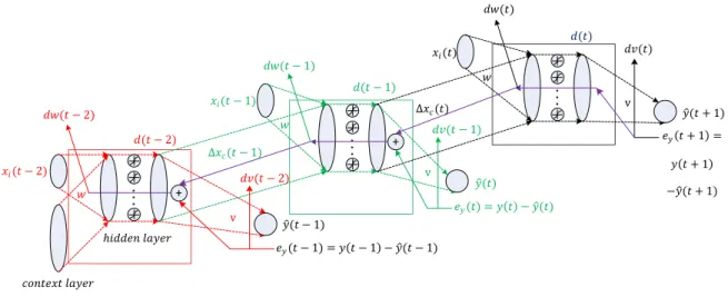
𝑦 (𝑡) 𝑥𝑖(𝑡 − 1) 𝑥𝑖(𝑡) 𝑒𝑦(𝑡) = 𝑦 𝑡 − 𝑦 (𝑡) 𝑑𝑣(𝑡 − 2) 𝑑𝑣(𝑡 − 1) 𝑑𝑣(𝑡) ℎ𝑖𝑑𝑑𝑒𝑛 𝑙𝑎𝑦𝑒𝑟 v 𝑤 v 𝑦 (𝑡 + 1) 𝑒𝑦 𝑡 + 1 = 𝑦 𝑡 + 1 −𝑦 (𝑡 + 1) 𝑤 v + 𝑦 (𝑡 − 1) 𝑥𝑖(𝑡 − 2) 𝑒𝑦(𝑡 − 1) = 𝑦 𝑡 − 1 − 𝑦 (𝑡 − 1) 𝑐𝑜𝑛𝑡𝑒𝑥𝑡 𝑙𝑎𝑦𝑒𝑟 𝑤 + 𝑑𝑤(𝑡) 𝑑𝑤(𝑡 − 1) 𝑑𝑤(𝑡 − 2) ∆𝑥𝑐(𝑡) ∆𝑥𝑐(𝑡 − 1) 𝑑(𝑡 − 1) 𝑑(𝑡 − 2) 𝑑(𝑡)
Fig. 3: The working principle of the back-propagation through time. A two step unfolded network showing back propagation of error at timet.
C. Training of the Elman Network
Before using, the network needs to be trained with a known sequence of input and its corresponding output. The training of the Elman network is different from the training of the canonical NN. It requires unfolding of the recurrent network to basic networks and back-propagation is applied on those networks. This special method is known as back-propagation through time (BPTT) [15].
1) Basic back-propagation: Back-propagation is a very simple and effective tool for training a non-recursive network. The known sequence is fed in the network and an output is found. The output is compared with the expected output and the error ey is determined. The error is fed back to the
network and the contribution of different parts i.e. ed, andea
are calculated. Then the weights are updated according to the contributions. It can be done in batch processing, i.e. the errors are summarized for all training samples and the weights are updated with that. The process is described in the following set of equations. ey=y−ˆy ed=vTey ean=dn(1−dn)edn forn= 1...N ∆v=γm∆v+γgeydT ∆w=γm∆w+γgeaxTF v=v+∆v w=w+∆w (2)
Here,γg, andγm are the learning gain and the momentum
gain respectively. γg determines how fast the network should
learn from one sample of the training sequence. On the other hand,γm determines the rigidity of the network to changes.
2) Back-propagation through time: Due to the recurrent nature of the Elman network, the training is different. BPTT is
an offline process of training the recurrent networks. A simple training method is shown in Fig. 3.
To integrate the effects of previous input, the network is unfolded upto a certain times, h. This is the depth of the network. In Fig. 3, the process of BPTT is shown forh= 3. For a single timet, the inputs are fed forxi(t−2),xi(t−1),
andxi(t). The weightsw, andvremain the same throughout
the forward process. The error for prediction of the last stage
ey(t+ 1) is fed back to updatev, andw. Forv, the update
is similar to (2). However, as w is affected by the values of
d, the values ofed(t−1) will be affected with both∆d(t),
andey(t). If∆xF(t)represents the corresponding change of
input, from the gradient based analysis, the expression of it is found as follows,
∆xF(t) =eTa(t)w (3)
∆xc(t)is the part of∆xF(t)corresponding to the context
layer. It gets added with the effect ofey to form the complete
effect ond(t−1),
ed(t−1) =∆xc(t) +vTey(t) (4)
The process runs till the starting network and the necessary corrections are determined. Then the last one of them are used to update the values ofw andv.
III. PREDICTION ANDTHELATESTTECHNOLOGIES
There is an important relation between the rate of data collection and the effectiveness of the predictor. Only one step ahead prediction is useless for a fast collection rate. It is discussed in the following section.
A. Nature of the States
In the traditional SCADA system, measurements are taken at a very slow rate of around 1 sample per 2-4 seconds. Under this rate, the collected samples miss some important changes
and they may look random. So, the use of the static WLS estimator is logical for this rate.
However, the estimator is getting faster day by day, and it requires a faster rate of collection of data. With the slowest PMU rate, i.e., 30 samples per second, the measurements show a complete dynamic nature. From the actual values of some simulations under different situations, it is observed that the states never change abruptly except the case of a fault. Even during a fault, they do not reach the final value within one sample. The actual values of the voltage magnitude of a bus of 16-machine 68-bus NY-NE system are shown in Figure 4.
Measurements taken at 1 sample per 2 seconds
10 20 30 40 50 60 70 80 90 100
Volatge magnitude of bus 25 0.9 0.95 1 1.05
Measurements taken at 30 samples/second
10 20 30 40 50 60 70 80 90 100
Voltage magnitude of bus 25 0.9 0.95 1 1.05
Fig. 4: The trend of one state under two different sampling rates. The upper one is taken at SCADA rate where the lower one presents the PMU rate.
As the SCADA rate cannot explore the dynamic natures of the states, a predictor becomes unsuitable for the purpose. With PMU rate, it can be an important part of the system.
B. Application of the state predictor
Any time ahead prediction can be helpful in the operation of the power system. The number of time steps depends on the time needed for the operator to take any action. Different actions require different amount of time to be taken. As a result, multiple predictor can run with different time steps to serve different purposes. It is important to remember that the accuracy of the prediction depends on the time step. If the prediction time is longer, the accuracy reduces.
The main application of the predictor can be in state estimation, contingency analysis, load forecasting, automatic voltage regulation, load frequency control, automatic genera-tion control, economic dispatch etc.
IV. TESTPOWERSYSTEM
The efficiency of the proposed predictor is tested in IEEE 16-machine 68-bus NY-NE test system. It has a total of 135 states with 83 transmission lines as shown in Fig. 5. For each bus, there are two computation cells for estimating the
magnitude and the angle as shown in Fig. 6. As a result, there exists a total of 135 ERNN cells which are separate from each other. They take the states of all neighboring cells. The states are taken directly from the simulation of the 68-bus system in Real Time Digital Simulator. In practice, they can be taken from the state estimator.
A. Training Data
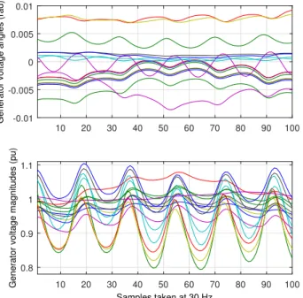
For both the single-step and the multi-step predictions, the training is done with 20000 data sampled at 30 Hz from the simulation of the system. The samples are iterated over 100-500 epochs to fit the training signals properly. To ensure a good amount of disturbance in the system, pseudo random binary signals (PRBS) are applied in the excitation control of the generators while collecting the measurements. A part of the 16 PRBS signals for 16 generators is shown in Fig. 7. The random changes take randomness in the training signals. The corresponding changes in the outputs of the generators are shown in Fig. 8.
The voltage magnitudes and the angles are separated. So, for each cell, there are two separate networks at each cell. Each cell uses the previous values of the corresponding state as well as the current value of it to predict the next value. If it predicts fornstep ahead result, it uses the previous values oft−tn andt−2tn. For the neighbors, it only uses the data
of current values.
The number of hidden layer neurons are taken to be double of the input layer. The number of the neurons of the context layer is equal to that of the hidden layers. As the network of each cell is producing either the magnitude or the angle, there is only one output neuron for each network.
The context layer is initialized with random weights. The starting inputs for this layer are zeros. As shown in Fig. 2, there is a one step delay between the output and the input part of the context layer.
B. Testing Data
The testing is done with 15428 samples of data taken under the same condition as of the training data. It is also initiated with zero values in the context layer. Though it gives some incorrect results in the beginning, the effects wear out very soon.
V. SIMULATIONRESULTS
Accuracy is the most important quality of any predictor. Though the accuracy of the voltage magnitude is well enough, the angles suffer a lot. The reason is the very low variation of phase angles over time. It makes the tracking difficult for the predictor.
To measure the accuracies of the predictors, Mean Absolute Percentage Error (MAPE) is taken for a single state over a specific number of time samples. MAPE is defined as,
M AP E= 1 n n X t=1 |Vjt−Vˆjt Vjt ×100%| (5)
Here, MAPE is taken overntime steps for busj.Vjt, and ˆ
Vjtrepresents the true and predicted value of the
9 36 4 6 17 19 1 47 48 40 41 66 14 10 15 16 11 12 13 3 2 6 7 5 4 9 8 1 42 67 52 68 49 46 62 31 30 32 63 33 38 34 35 45 51 50 39 44 64 37 43 65 3 2 8 7 5 54 27 18 16 25 26 28 29 61 53 60 24 21 22 23 58 59 55 56 57 14 13 12 11 10 15 20 Area 1 Area 2 Area 3 Area 5 Area 4
New England Test System New York Power System
Fig. 5: IEEE 68-bus NY-NE test system.
V2(t-2tn) V2(t-tn) V2(t) V1(t) V3(t) V25(t) V52(t) V2(t+tn) ERNN cell for the magnitude of bus 2 θ2(t-2tn) θ2(t-tn) θ2(t) θ1(t) θ3(t) θ25(t) θ52(t) θ2(t+tn) ERNN cell for the angle of bus 2
Fig. 6: Inputs and outputs for the two cells of bus 2.
A. Single step prediction
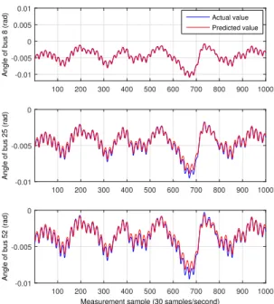
The accuracy is important for both the training session as well as for the testing session. With a repetition of 100-500 epochs, the training session usually gets an acceptable accuracy as shown in Fig. 9. For the testing session, the accuracies of the phase angles and the voltage magnitudes of bus 8, 25, and 52 are shown in Figs. 10, and 11. These are carried out for a single step prediction.
Samples taken at 30Hz
10 20 30 40 50 60 70 80 90 100
Magnitudes of the 16 PRBS signals
-0.2 -0.15 -0.1 -0.05 0 0.05 0.1 0.15 0.2
Fig. 7: PRBS signals used to perturb the generators in the power system.
B. Multi-step prediction
As the single step prediction is not suitable for some operations, multi-step predictions are needed. The training is done for multiple steps and the testing is shifted accordingly. The inputs are shifted according to the step size. For example, if the step size is six, the previous values are taken from
t−6 andt−12. It is found that the multi-step prediction is less accurate than the single step prediction. A six step ahead prediction results are shown in Figs. 12, and 13.
10 20 30 40 50 60 70 80 90 100 Generator voltage angles (rad) -0.01
-0.005 0 0.005 0.01 Samples taken at 30 Hz 10 20 30 40 50 60 70 80 90 100
Generator voltage magnitudes (pu)
0.8 0.9 1 1.1
Fig. 8: The output of the generator voltages due to the PRBS signals.
Sample number ×104 1.57 1.58 1.59 1.6 1.61 1.62
Angle of bus 25 (rad)
0.16 0.18 0.2 0.22 0.24 0.26 0.28 0.3 0.32 0.34 0.36 Actual value Predicted value
Fig. 9: A part of the final training values and the predicted training values.
prediction error (STD) for the single and the multi-step pre-dictions are shown in Table 1.
TABLE I
MAPE±STDFORPREDICTIONS
Bus Single-step Six-step
|V| θ |V| θ
8 0.77±0.61 3.48±2.29 1.84±1.21 16.5±15.4
25 0.85±0.57 3.81±2.42 2.41±1.52 15.5±12.9
52 0.55±0.39 6.81±4.37 2.19±1.27 24.4±31.4
VI. CONCLUSION
A CCN inspired ERNN based dynamic state predictor is proposed for power systems and the simulation results are shown in this study. The results show that the network works well for the single state prediction. The accuracy of the multi-step predictor is also satisfactory.
The fully connected CCN is left as the future work. The single step prediction can be effectively used for distributed dynamic state estimation. It is also left as a future work. The relation between the step size and the accuracy of the predictor is also an important area of research. Though not explored, the accuracy may get better with some periods of steps.
REFERENCES
[1] A. Abur and A. Exposito,Power System State Estimation: Theory and Implementation. New York, NY: Marcel Dekker Inc., 2004.
[2] F. D. Galiana, “Bound estimates of the severity of line outages in power system contingency analysis and ranking,”IEEE Trans. Power Apparatus and Systems, no. 9, pp. 2612–2624, 1984.
[3] D. C. Park, M. El-Sharkawi, R. Marks, L. Atlas, M. Damborget al., “Electric load forecasting using an artificial neural network,” IEEE Trans. Power Systems, vol. 6, no. 2, pp. 442–449, 1991.
[4] J. Stewart, T. Maufer, R. Smith, C. Anderson, and E. Ersonmez. (2016, January) Synchrophasor security practices. [Online]. Avail-able: https://cdn.selinc.com/assets/Literature/Publications/Technical% 20Papers/6449_SynchrophasorSecurity_EE_20100913_Web.pdf [5] Z. Huang, K. Schneider, and J. Nieplocha, “Feasibility studies of
apply-ing kalman filter techniques to power system dynamic state estimation,” in International Power Engineering Conference, 2007, Dec 2007, pp. 376–382.
[6] K. Balasubramaniam, G. K. Venayagamoorthy, and N. Watson, “Cellular neural network based situational awareness system for power grids,” in
The 2013 International Joint Conference on Neural Networks (IJCNN),. IEEE, 2013, pp. 1–8.
[7] ——, “Situational awareness system for power grids,” Graduate Re-search and Discovery Symposium (GRADS), 2013, paper 61. [8] M. R. Qader, M. H. Bollen, and R. N. Allan, “Stochastic prediction
of voltage sags in a large transmission system,”IEEE Transactions on Industry Applications, vol. 35, no. 1, pp. 152–162, 1999.
[9] B. L. Smith and M. J. Demetsky, “Short-term traffic flow prediction: neural network approach,” Transportation Research Record, no. 1453, 1994.
[10] M. D. Odom and R. Sharda, “A neural network model for bankruptcy prediction,” in IJCNN International Joint Conference on neural net-works, 1990, pp. 163–168.
[11] D. Kneller, F. Cohen, and R. Langridge, “Improvements in protein secondary structure prediction by an enhanced neural network,”Journal of molecular biology, vol. 214, no. 1, pp. 171–182, 1990.
[12] P. Rousseaux, D. Mallieu, T. V. Cutsem, and M. Ribbens-Pavella, “Dynamic state prediction and hierarchical filtering for power system state estimation,” Automatica, vol. 24, no. 5, pp. 595 – 618, 1988. [Online]. Available: http://www.sciencedirect.com/science/article/ pii/0005109888901082
[13] B. Luitel and G. K. Venayagamoorthy, “Cellular computational networks—A scalable architecture for learning the dynamics of large networked systems,”Neural Networks, vol. 50, pp. 120–123, 2014. [14] J.-G. Wu and H. Lundstedt, “Prediction of geomagnetic storms from
solar wind data using Elman recurrent neural networks,” Geophysical research letters, vol. 23, no. 4, pp. 319–322, 1996.
[15] P. J. Werbos, “Backpropagation through time: what it does and how to do it,”Proceedings of the IEEE, vol. 78, no. 10, pp. 1550–1560, 1990.
100 200 300 400 500 600 700 800 900 1000 Angle of bus 8 (rad) -0.01
-0.005 0 0.005 0.01 Actual value Predicted value 100 200 300 400 500 600 700 800 900 1000
Angle of bus 25 (rad)
-0.01 -0.005 0
Measurement sample (30 samples/second)
100 200 300 400 500 600 700 800 900 1000
Angle of bus 52 (rad)
-0.01 -0.005 0
Fig. 10: A part of the testing values and the predicted testing values for a single step prediction of phase angle.
100 200 300 400 500 600 700 800 900 1000 |V| of bus 8 (pu)0.9 1 1.1 1.2 Actual value Predicted value 100 200 300 400 500 600 700 800 900 1000 |V| of bus 25 (pu) 0.8 0.9 1 1.1
Measurement sample (30 samples/second)
100 200 300 400 500 600 700 800 900 1000 |V| of bus 52 (pu)0.9
1 1.1
Fig. 11: A part of the testing values and the predicted testing values for a single step prediction of voltage magnitude.
100 200 300 400 500 600 700 800 900 1000
Angle of bus 8 (rad)
×10-3 -10 -5 0 5 Actual value Predicted value 100 200 300 400 500 600 700 800 900 1000
Angle of bus 25 (rad)
-0.01 -0.005 0
Measurement sample (30 samples/second)
100 200 300 400 500 600 700 800 900 1000
Angle of bus 52 (rad)
-0.01 -0.005 0
Fig. 12: A part of the testing values and the predicted testing values for a six step prediction of phase angle.
100 200 300 400 500 600 700 800 900 1000 |V| of bus 8 (pu)0.9 1 1.1 1.2 Actual value Predicted value 100 200 300 400 500 600 700 800 900 1000 |V| of bus 25 (pu) 0.8 0.9 1 1.1
Measurement sample (30 samples/second)
100 200 300 400 500 600 700 800 900 1000 |V| of bus 52 (pu) 0.8 0.9 1 1.1
Fig. 13: A part of the testing values and the predicted testing values for a six step prediction of voltage magnitude.