Lutz Gross, Hans M¨
uhlhaus, Elspeth Thorne and Ken Steube
Abstract. In this paper we continue the development of our python-based package for the solution of partial differential equations using spatial dis-cretization techniques such as the finite element method (FEM), but we take it to a higher level using two approaches: First we define a Model class ob-ject which makes it easy to break down a complex simulation into simpler sub-models, which then can be linked together into a highly efficient whole. Second, we implement an XML schema in which we can save an entire simu-lation. This allows implementing check-pointing and also graphical user inter-faces to enable non-programmers to use models developed for their research. All this is built upon our escript module, which makes it easy to develop numerical models in a very abstract way while using the computational com-ponents implemented in C and C++ to achieve extreme high-performance for time-intensive calculations.Keywords.Partial Differential Equations, Mathematical Modelling, XML schema, Drucker–Prager Flow.
1. Introduction
These days numerical simulation is a team effort combining a variety of skills. In a very simple approach we can identify four groups of people being involved: re-searchers using numerical simulation techniques to improve the understanding and predict phenomenas in science and engineering, modelers developing and validating mathematical models, computational scientists implementing the underlying nu-merical methods, software engineers implementing and optimizing algorithms for a particular architecture. Each of these skill levels uses their individual terminology: researcher is using terms such stress, temperature and constitutive laws, while the modeler is expressing his models through functions and partial differential equations. The computational scientist is working with grids, matrices. Software engineers is working with arrays and data structures. Finally, an object such as stress used by a researcher is represented as a suitable, maybe platform dependent,
data structure after the modeler has interpreted as a function of spatial coordi-nates and the computational scientists as values at the center of elements in a finite element mesh. When moving from the software engineer’s view towards the view of the researcher the data structures undergo an abstraction process finally only seeing the concept of stress but ignoring the fact that it is a function in the
L2
Sobolev space and represented by using a finite element mesh.
It is also important to point out that each of these layers has an appropriate user environment. For the researcher, this is a set input files describing the prob-lem to be solved, typically in XML [5]. Modelers, mostly not trained as software engineers, prefer to work in script-based environments, such as python [7] while computational scientists and software engineers are are working in C and C++ to achieve best possible computational efficiency.
Various efforts have been made to provide tools for computational scientists to develop numerical algorithms, for instance PETSc [13] which is widely used. These tools provide linear algebra concepts such as vectors and matrices and hid-ing data structures from the user. The need of researchers for an easy to use environment has been addressed through various developments in problem solving environments (PSEs) [8] which is some case can be a simple graphical user inter-face. There were only a rather small number of activities towards environments for modelers. Two examples for partial differential equation (PDE) based mod-elling are ELLPACK [11] and FASTFLO [12]. Both products are using there own programming language which is not powerful enough to deal with complex and coupled problems in an easy and efficient way.
Theescript module [1, 2] which embedded into python is an environment in which modelers can develop PDE based models. It is designed to solve general, coupled, time-dependent, non-linear systems of PDEs. It is a fundamental design feature of escript that is not tight to a particular spatial discretization technique or PDE solver library. It is seamlessly linked with other tools such as linear algebra tools [14] and visualization tools [15].
In this paper we will give an overview into the basic concepts of escript
from a modellers point of view We will illustrate its usage for implementing the Drucker–Prager flow model. In the second part we will present the modelframe
module withinescript. It provides a framework to implement mathematical models as python objects which then can be plugged together to build simulations. We illustrate this approach for the Drucker–Prager flow and show how this model can be linked with a temperature advection–diffusion model without modifying the codes for any of the models. We will then discuss how XML can be used to set simulation parameters but also to define an entire simulation from existing models. The XML files provide an ideal method to build simulations out of PSEs or from web services. The presented implementation of the Drucker-Prager flow has been validated on some test problems but as it not the purpose of the paper to discuss models no results are presented.
2. Drucker–Prager Flow Model
2.1. The General FrameworkWe will illustrate the concepts for the deformation of a three-dimensional body loaded by the time-dependent volume force fi and by the surface load gi. If ui
andσij defines the displacement and stress state at a given time tand dtgives a
time increment the general framework for implementing a model in the updated Lagrangian framework is given in the following form:
0. start time integration, sett= 0 1. start iteration at timet, setk= 0
1.0. calculate displacement incrementdui from σ
−
ij and current forcefi.
1.1. update geometry
1.2. calculate stretchingDij and spinWij fromvi.
1.3. calculate new stressσij fromσ
−
ij using Dij and Wij.
1.4. update material properties from σij
1.5. if not converged,k←k+ 1 and goto 1.0. 2. sett←t+dtand goto 1.
The superscript 0
−0
refers to values at the previous iteration or time step. To terminate the iteration process at a time step one can use the relative changes in the velocityvi= u−u
−
dt :
kduk∞≤ζiterkuk∞ (2.1)
where k.k∞ denotes the maximum norm andζiter is a given positive relative
tol-erance. Alternatively, one can check the change stress.
The keep the relative time integration error below the given toleranceζtime
the time stepdt for the next time step should be kept belowdtmax given by
dtmax=
dtkuk∞
kv−v−k ∞
ζtime. (2.2)
which controls an estimate of the local time discretization error for the total dis-placementu.
The stretchingDijand spinWijare given as the symmetric and non-symmetric
part of the the gradient ofdui:
Dij = 1 2(dui,j+duj,i) (2.3) Wij = 1 2(dui,j−duj,i) (2.4)
where where for any functionZ Z,idenotes the derivative ofZ with respect toxi.
To calculate the displacement increment dui one has to solve a partial
dif-ferential equation on the deformed domain Ω−
which takes in tensor notation the form −(Sijklduk,l),j = (σ − ij−K thδ ij),j+fi (2.5)
where K is the bulk modulus and Sijkl is the tangential tensor which depends
hand side is the Cauchy stress at timet−dtwith the mechanical stressσ−
ij at time
t−dt. The termK thδ
ij is the thermal stress where the thermal volume strain
this given as
th=θ(T−Tref) (2.6)
with thermal expansion coefficientθand current temperatureT and the reference temperature Tref. In geoscience applications, fi typically takes the form of the
gravitational force
fi=−ρ gδid (2.7)
which acts oppositely to the positive ddirection. The constants g is the gravity constant andρis the density which is often given in the form
ρ=ρ0(1−θ(T−T0)) (2.8) whereρ0 is the density at reference temperatureT0.
The displacement increment has to fulfill the conditions
nj(Sijklduk,l+σ
−
ij−K thδij) =gi (2.9)
on the boundary of the domain wheregiis a possibly time-dependent surface load.
Moreover, the displacement increment has to meet a constraint of the form
du=dt·Vi on Γi (2.10)
where Γi is a subset of the boundary of the domain. At the first iteration stepVi
gives thei-th velocity component acting at the subset Γi of the deformed domain
and is set to zero for the following steps. 2.2. The Drucker-Prager Model
For the Drucker-Prager Model the stress update is done in the following way: First the stress state at time t+dtdue to elastic deformationσe
i,j is calculated: σije =σ− ij+K thδij+dt 2G Dij+ (K− 2 3G)Dkkδij+Wikσ − kj−σ − ikWkj (2.11) whereGis the shere modulus. Then Based on the elastic trial stressσe
i,j the yield
functionF is obtained as The yield function is evaluated
F =τe−α pe−τY (2.12) where pe=−1 3σ e kk (2.13) τe= r 1 2(σ e ij) 0(σe ij) 0 (2.14)
with the deviatoric stress
(σije)0
=σije +peδij. (2.15)
The valueτY is current shear length andαis the friction parameter which both
We want to have the yield function to be non-negative. The factorχ marks when the yield condition is violated:
χ=
0 forF <0
1 else (2.16)
With current hardening modulus h = dτY
dγp and dilatency parameter β, which is again a given function of the plastic shear stressγp, we set the plastic shear stress
increment to
λ=χ F
h+G+βK (2.17)
We then can calculate a new stress as
τ =τe−λG (2.18) σij= τ τe(σ e ij) 0 −(pe+λβK)δij (2.19)
Finally we can update the plastic shear stress
γp=γp−
+λ (2.20)
and the harding parameter
h= τY −τ
−
Y
γp−γp− (2.21)
For the Drucker-Prager model the tangential tensor is given as
Sijkl = G(δikδjl+δjkδil) + (K− 2 3G)δijδkl +(σ− ijδkl−σ − ilδjk) + 1 2(δikσ − lj−δjlσ − ik+δjkσ − il −δilσ − kj) − χ h+G+αβK G(σij)0 τ +βKδij G(σkl)0 τ +αKδkl (2.22)
When implementing the model we have to keep track of the total stressσ, plastic stressγp, the shear lengthτ
Y as well as displacementuand velocityv.
It is also important to keep in mind that the model is temperature-dependent through the thermal strain and through the temperature-dependent density as well as the standard advection-diffusion equation, the so called heat equation [4].
3. Implementation
The key problem in the Drucker-Prager model is to solve a linear, steady partial differential equation. The coefficients of the PDE are given by arithmetic expres-sions of the PDE solutions. In this chapter we outline the concept of the python
3.1. Spatial Functions
The solution of a PDE as well as the PDE coefficients are functions of the spatial coordinates varying within a domain. In escript a domain is represented in a
Domainclass object. TheDomainclass object does not only hold information about the geometry of the domain but also about a PDE solver library that is used to solve PDEs on this Domain. In particular, the Domain class object defines the discretization technique, such as finite difference method (FDM) or finite element method [3], which is used to represent spatial functions on the domain. In the current implementation escript is linked to FEM solver libraryfinley [2] but the design is open and other libraries could be implemented.
A spatial function is represented through its values on sample points. For instance, in the context of the FEM the solution of a PDE is represented by it values on the nodes while PDE coefficients are typically represented by their values at the element centres. The appropriate representation of a function is chosen by
escript but, if required, can be controlled by the user.
Spatial functions can be manipulated by applying unary operations, for instance cos, sin, log) and be combined through binary operations, for ininstance +, -,* , /. When combining spatial functions with different representationsescriptuses interpolation to make the representations of the arguments compatible for combi-nation. If in the FEM context a function represented by it values on the element centers and a function represented by it values on the nodes is added together, interpolation from nodes to element centers will be performed before the addition takes place.
In the current version of escript, three internal storage schemes for spatial function representation are used. In the most general case individual values are stored for each sample point. Typically this expanded storage scheme is used for the solution of a PDE. In many cases PDE coefficients are constant. In this case, it would be a waste of memory and compute time to use the expanded storage scheme. For this caseescript stores a single value only and refers to this value whenever the value for a sample point is requested. The third form represents piecewise constant functions which are stored as a dictionary. The keys of the dictionary refer to tags assigned to the sample points at the time of mesh generation. The value at a sample point is accessed via the tag assigned to sample point and the associated value of the tag in the dictionary. Typically, this technique is used when a spatial function is defined according to its location in certain subregions of the domain, for instance in the region of a certain rock type. When data objects using different storage schemes are combined,escript chooses an appropriate storage scheme in which to store the result.
The following python function implements stress update for the Drucker-Prager model as presented in section 2.2. It takes the last stress σ−
ij (=s_old),
the last plastic stress γp−
(=gamma_p_old), displacement increment dui (=du),
the thermal volume strain increment th (=deps_th) and the relevant material
from escript import * def getStress(du,s,gamma_p_old,deps_th,tau_Y,G,K,alpha,beta,h): g=grad(du) D=symmetric(g) W=nonsymmetric(g) s_e=s+K*deps_th*kronecker(3)+ \ 2*G*D+(K-2./3*G)*trace(D)*kronecker(3) \ +2*symmetric(matrix_mult(W,s) p_e=-1./3*trace(s_e) s_e_dev=s_e+p_e*kronecker(3) tau_e=sqrt(1./2*inner(s_e_dev,s_e_dev)) F=tau_e-alpha*p_e-tau_Y chi=whereNonNegative(F) l=chi*F/(h+G+alpha*beta*K) tau=tau_e-l*G s=tau/tau_e*s_e_dev+(p_e+l*beta*K)*kronecker(3) gamma_p=gamma_p+l return s, gamma_p
Each of the arguments, with the exception of v, can be a python floating point number or anescript spatial function. The argumentvmust be an escript spatial function. The Domain attached to it is the Domain of the returned values. Their representations are determined by the grad call, which returns the gradient of its argument. In the FEM context, the argument ofgradmust be represented by its values on the nodes while the result ofgradis represented by its values at the element centers. This representation is carried through to the return values. Notice that this function does not depend on whether values are stored on the nodes or at the centers of the elements, and so it may be re-used without change in any other model, even a finite difference model.
3.2. Linear PDEs
The LinearPDE class object provides an interface to define a a general, second order, linear PDE. TheDomainclass object attached to aLinearPDEclass object defines the domain of the PDE but also defines the PDE solver library to be used to solve the PDE.
The general form of the PDE for an unknown vector-valued functionui
rep-resented by theLinearPDEclass is
−(Aijkluk,l+Bijkuk),j+Cikluk,l+Dikuk=−Xij,j+Yi (3.1)
The coefficientsA,B,C,D,XandY are functions of their location in the domain. Moreover, natural boundary conditions of the form
nj (Aijkluk,l+Bijkuk−Xij,j) =yi (3.2)
can be defined. In this condition, (nj) defines the outer normal field of boundary of
of the domains one can define constraints of the form
ui=ri whereqi>0 (3.3)
whereqiis a characteristic function of the locations where the constraint is applied.
From inspecting equation 2.5 and equation 2.9 we can easily identify the value for the PDE coefficient to calculate the displacement incrementdui:
Aijkl=Sijkl, Yi=fi, X =σ
−
ij−K thδ
ij andyi=gi. (3.4)
The constraints fordui, see equation 2.10 is defined by
ri=dt·Vi andqi(x) =
1 forx∈Γi
0 otherwise (3.5)
If the functiongetTangentialTensorreturns the tangential operator, the follow-ing function returns a new displacement incrementduby solving a linear PDE for theDomainclass objectdom:
from escript import LinearPDE
def getDu(dom,dt,s,dt,deps_th,tau_Y,G,K,alpha,beta,h,f,g,Gamma,V): pde=LinearPDE(dom) S=getTangentialTensor(s,tau_Y,G,K,alpha,beta,h) pde.setValue(A=S, X=s-K*deps_th*kronecker(3), \ Y=f, y=g) pde.setValue(q=Gamma, r=dt*V) du=pde.getSolution() return du
It would be more efficient to create one instance of the LinearPDEclass object and to reuse it for each new displacement increment with updated coefficients. This way information that are expensive to obtain, for instance the pattern of the stiffness matrix, can be preserved. The following function returns the tangential tensorS:
from escript import *
def getTangentialTensor(s,,tau_Y,G,K,alpha,beta,h): k3=kronecker(3) p=-1./3*trace(s) s_dev=s+p*k3 tau=sqrt(1./2*inner(s_dev,s_dev)) chi=whereNonNegative(tau-alpha*p-tau_Y) tmp=G*s_dev/tau sXk3=outer(s,k3) k3Xk3=outer(k3,k3) S= G*(swap_axes(k3Xk3,0,3)+swap_axes(k3Xk3,1,3)) \ + (K-2./3*G)*k3Xk3 \ + (sXk3-swap_axes(swap_axes(sXk3,1,2),2,3)) \ + 1./2*( swap_axes(swap_axes(sXk3,0,2),2,3) \ -swap_axes(swap_axes(sXk3,0,3),2,3) \
-swap_axes(sXk3,1,2) \
+swap_axes(sXk3,1,3) ) \
- outer(chi/(h+G+alpha*beta*K)*(tmp+beta*K*k3),tmp+alpha*K*k3) return S
The values chi, s_devand tau calculated in a call of getStresscould used in this calculation of the new stress could be reduced ingetTangentialTensor.
4. Modelling Framework
From the functions presented in the previous section 3 one can easily build a time integrations scheme to implement a Drucker-Prager flow model through two nested loops. The outer loop progresses in time while the inner loop iterates at time step until the stopping criterion (2.1) is fulfilled. The time step size is con-trolled by criterion 2.2. This straight-forward approach has the drawback that the code has to modified when the temperature dependence becomes time-dependent. Then a advection-diffusion model for the temperature has to be worked into the code which may use a different time step size. In addition, the thermal strainth
is changing over time but also material parameters, for instance density, see equa-tion (2.8), may become temperature-dependent. The coding effort to implement these components is not large but has the big drawback that the submodel, such as the Drucker-Prager model, the temperature advection-diffusion model and the material property tables, loose their independence. However, from a software de-velopment point of view it is highly desirable to keep the models independent in order to test and maintain them separately and reuse models in another context. 4.1. Linkable Objects
To resolve this problem, a model, such as Drucker-Prager flow model, is imple-mented in a python class. Model parameters, such as external force Fi or state
variables, such as stress σij, are defined as object attributes. For instance if the
classDruckerPragerimplements the Drucker–Prager flow andGravitythe grav-ity force (2.7) one uses
g=Gravity() g.density=1000 flow=DruckerPrager() flow.force=g.force
to assign a value to the density of the gravity force and then defines the gravity force as the external force of the Drucker–Prager flow model. In the case of con-vection model, the density is not constant but calculated from a temperature field updated through the temperature model over time. However, theGravityobject
g has to use the most recent value of the density at any time of the simulation. To accomplish this theescript module provides two classesLinkableObjectsand
Link. A Linkclass object is a callable object that points to an attribute of the target object. IfLinkclass object is called the current value of the attribute of the
target object is returned. If the value is callable, the value is called and the result is returned. So, similar to a pointer in C, aLinkclass object defines another name for a target value, and is updated along with the target object.
ALinkableObjectsclass object is a standardpython object with a modified
__getattr__method: when accessing its attributes it behaves like a usualpython
object except if the value is aLinkclass object. In this case, the link is followed, that means the value is called and the result returned. The mechanism allows to link an attribute ofLinkableObjectsclass object with the attribute of another target object such that at any time the object uses the value of the target object. The following script shows how a gravity force in flow model can be defined where the density of the gravity model is temperature-dependent:
mat=MaterialTable() mat.T_0=20 temp=Temperature() g=Gravity() flow=DruckerPrager() mat.T=Link(temp,"temperature") g.density=Link(mat,"rho") flow.force=Link(g,"force")
The four classesMaterialProperties Temperature,GravityandDruckerPrager
implementing a material property table, a temperature advection-diffusion model, a gravity force model and a Drucker-Prager flow model. The temperature parame-terTof the material property table is provided by the temperature model attribute
temperature. The densityrhoprovided by the material property table is fed into the gravity model which then provides the external force for the flow model.
The model (2.8) of a temperature-dependent density can be implemented in the following way:
class MaterialProperties(LinkableObject): def rho(self):
return self.rho_0*(1.-self.theta*(self.T-self.T_0))
If the temperatureTis linked to a time-dependent temperature model via aLink
object the method rhowill always use the most recent value of the temperature even if it is updated by the target temperature model. On the other hand, if an attribute of another model, for instance the attributedensityof aGravityclass object, is linked against the methodrhoof an instance of theMaterialProperties
class, accessing the attribute will call the the methodrhoand use its return value calculated for the current temperature. Through the chain of links the Drucker-Prager flow model is coupled with the temperature modules. It is pointed out that if the temperature model considers advection, the velocity updated by Drucker-Prager flow model is referenced by the temperature model which produces a loop of references requiring an iteration on a time step.
4.2. Models
Implementing models asLinkableObjectclass objects solves the problem of defin-ing the data flow of coupled models but we also need an execution scheme for individual models in order to be able to execute a set of coupled models with-out changing any of involved models. An appropriate execution scheme is defined through the Modelclass of the modelframe module. The Modelclass which is a subclass of the LinkableObjectclass provides a template for a set of methods that have to be implemented for a particular model. TheModelclass methods are as follows:
• doInitialization: This method is used to initialize the time integration process. For the flow model this method initializes displacements and stress for time t = 0 and to create an instance of the LinearPDE object used to update the displacement through equation (2.5).
• getSafeTimeStepSize: This method returns the maximum time step size that can be used to safely execute the next time step of the model. For the flow model the time step size defined by condition (2.2)) is returned. • doStepPreprocessing: This method prepares the iterative process to be
ex-ecuted on a time step. Typically, this function will set an initial guess for the iterative process to run on a time step.
• doStep: This method performs a single iteration step to update state variables controlled by the model due to changes in input parameters controlled by other models. For the Drucker–Prager flow model thedoStepperform a single iteration step by solving the PDE (2.5) and updating the stress via (2.19). • terminateIteration: The method returnsTrueif the iterative process on a
time step can be terminated. Typically, a stopping criterion of the form (2.1) is checked.
• doStepPostprocessing: This method finalizes a time step, typically by shift-ing the current values of state variables into the buffer of the previous time step.
• finalize: The method returnsTrueis the time integration is finalized. Typ-ically this method checks the current time against a given end time.
• doFinalization: This method finalizes the whole modeling run, typically by closing files and cleaning up.
AnyModelclass object is run in the following way:
m=Model()
m.doInitialization() while not finalize():
dt=m.getSafeTimeStepSize(dt) m.doStepPreprocessing(dt)
while not m.terminateIteration(): m.doStep(dt) m.doStepPostprocessing(dt)
This scheme is executed by theSimulationclass, which will be discussed in the next section 4.3.
The following sub-class of the Model class implements the Drucker–Prager flow model: class DruckerPrager(Model): def doInitialization(self): self.pde=LinearPDE(self.domain) self.stress=Tensor(0.,Function(self.doamin)) self.displacement=Vector(0.,Solution(self.doamin)) self.velocity=Vector(0.,Solution(self.doamin)) self.t=0 def getSafeTimeStepSize(self): return dt*Lsup(u)/Lsup(self.velocity-self.velocity_old)*self.zeta def doStep(self,dt): S=self.getTangentialTensor() pde.setValue(A=S, X=self.stress,Y=self.force) self.du=self.pde.getSolution() self.displacement=self.displacement+self.du self.velocity=(self.displacement-self.displacement_old)/dt self.stress=self.getStress() def terminateIteration(self,dt): return Lsup(self.du)<=self.zeta*Lsup(self.displacement) def doStepPostprocessing(self,dt): self.velocity_old=self.velocity self.t+=dt def finalize(self): return self.t<self.t_end
OmittedModelclass methods are empty. The functionsgetStressandgetTangentialTensor
introduced in section 3.2 are turned into class methods. Function parameters are now accessed as class attributes.
4.3. Simulations
TheSimulationclass controls the execution of a list of submodels. It is an imple-mentation of theModelclass, where eachModelmethod executes the corresponding method of all the submodels: ThegetSafeTimeStepSizereturns the minimum of all step sizes required by the submodels. If all submodels terminate their iterative process terminateIterationreturnsTrue. The simulation is terminated by the
finalizemethod if any of the submodels is to be finalized. ThedoStep method iterates over all submodels until all submodel indicate convergence.
The following script outlines the usage of theSimulationclass for construct-ing and runnconstruct-ing a coupled temperature diffusion and Drucker-Prager flow model:
mat=MaterialTable() temp=Temperature()
g=Gravity()
flow=DruckerPrager()
s=Simulation([temp,mat,g,flow]) s.run()
The couplings between the models as shown in section 4.1 have been omitted. The
runmethod of theSimulationclass executes its Modelmethods as shown in the previous section 4.2. At a time step, the simulation iterates over the submodels until all submodels have converged. The execution order is defined by the order of the models inSimulationclass argument. Alternatively, one can iterate over the flow model only and use the temperature from the previous time step. This can be achieved through
Simulation([temp,mat,g,Simulation([flow])).run()
where the convergence tolerance in the temperature model has to be chosen appro-priately. Note that visualization functionality, for instance to create a movie of the velocity field, can be implemented as aModelclass where in thedoStepPostprocessing
method the velocity field is rendered after for each time step, while thedoFinalization
method creates the movie from the frames.
It is pointed that the coupling of the models does not require any knowledge of the algorithms being used to implement the model. Furthermore, the codes implementing a model are not altered to perform the coupling. The coupling is based purely on the submodel parameters. This high-level approach is possible because of the abstraction level that is provided by theescript environment.
5. Simulation and XML
Concurrent to the modeling framework, an XML dialect calledEsysXMLhas been developed with the objective to store simulations in a transportable form, to define the coupling of models and to allow the creation of dynamic templates of model interfaces.
5.1. XML Model Interface
The parameters used to link models are called external parameters, and are stored in a Model class object. These parameters may be set by the programmer or by another model. TheModelalso stores internal parameters used in the various methods implementing the model. For instance for theModelclassDruckerPrager
introduced in section 4.2domain,force, stress, displacementand velocity
are external parameters whilepdeandtare internal parameters that are unavail-able to other models. External parameters are exposed via thedeclareParameter
method called at Modelclass object initialization. For example, the Modelclass
DruckerPrageris written in the following way:
class DruckerPrager(Model): def __init__(self):
self.declareParameters(domain=None, force=0., \ stress=0., displacement=0., \ velocity=0.)
This explicit declaration restricts the necessary input and output parameters that are exposed on a user-interface level. The XML representation of a Modelclass object includes all parameters and their current values, which could beLinkclass objects. The python implementation of a model itself is not stored in XML, only the data and the links between models.
ASimulationclass object can be written into a XML file using the EsysXML. This includes all submodels, their external parameter and values and possibly links between the submodels. This file can be edited using any text editor to change value of external parameters, introduce new models and set or remove couplings between models. ASimulationclass object can be build from the XML file. The parser uses the standard python XML tools, packaged in PyXML [9]. Primarily,
minidom is used to parse and generate XML content. It is a lightweight, simple implementation of the standard Document Object Model (DOM) interface, and is fast. An important application of writingSimulationclass objects to XML is automated check-pointing.
5.2. Technical specifications of EsysXML
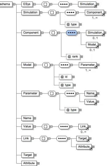
A diagram of the XML schema [6] used by EsysXML is included in Figure 1 at the end of this paper.
The XML begins with an Esys tag, which includes a single Simulation. ThatSimulationcontains one or more components, each of which may be either aModelor anotherSimulation. The ranks of theComponentobjects tell the order in which they are to be executed. Each Modelincludes one or more Parameter
objects defined by a type (float, string or Link) and the name and value of the parameter. Whether or not a parameter is internal or external (available to other models) is determined by the use ofdeclareParametersin the python script which implements the model.
The Link items, require that a persistent, deterministic way of preserving associations between linkedModelclass objects. This is achieved by generating a unique reference identification number for each Modelclass object which defines theidattribute. For aLinkitem theTargetXML attribute specifies the reference identification number of the targetModelitem while the XML attributeAttribute
specifies the name ofParameteritem of the targetModel.
6. Conclusion
The design we have chosen forescript simplifies the development of complex yet efficient models by breaking them down into a series of simpler steps. In the ex-ample above, we developed a Drucker-Prager flow model and a gravity model, and
then later on we linked them together with a temperature adevection-diffusion model to create a more complex simulation.
By modifying the standardpythonmechanism for accessing object attributes, we allow sharing values between models without creating any burden on the mod-eller. The sharing of parameters between models is very efficient due to our use of links.
By adding the ability to store an entire simulation in XML format we have created a new level of control over a model. Using this technique we will be able to check-point simulations, share simulations with collaborators, and also provide a Graphical User Interface, such as in a web page, to define the parameters of a simulation and adjust models in a simulation. Once a modeller has developed a simulation inpython it may then be used and adjusted by a researcher who is not burdened to do further programming.
Acknowledgment
Project work is supported by Australian Commonwealth Government through the Australian Computational Earth Systems Simulator Major National Research Facility and the Australian Partnership for Advanced Computing, Queensland State Government through the Smart State Research Facility Fund, The University of Queensland, the Queensland Cyberinfrastructure Foundation and SGI Ltd.
References
[1] Gross, L. and Cochrane, P. and Davies, M. and M¨uhlhaus, H. and Smillie J.: Es-cript: numerical modelling in python. Proceedings of the Third APAC Conference on Advanced Computing, Grid Applications and e-Research (APAC05),(2005).
[2] Davies, M. and Gross, L. and M¨uhlhaus, H. -B.: Scripting high-performance Earth systems simulations on the SGI Altix 3700.Proceedings of the 7th international con-ference on high-performance computing and grid in the Asia Pacific region, (2004). [3] Zienkiewicz, O. C. and Taylor, R. L.:The Finite Element Method. 5th Edition,
But-terworth Heinemann, (2000).
[4] R. E. Williamson: Differential Equations and Dynamical Systems, McGrawHall (2001).
[5] http://www.w3.org/XML/ (2006), [on-line].
[6] C. M. Sperberg-McQueen and H. Thompson: XML Schema, www.w3.org/XML/Schema (2006), [on-line].
[7] M. Lutz,Programming Python, 2nd EditionO’Reilly (2001).
[8] E. N. Houstis, E. Gallopoulos, J.R. Rice, R. Bramley:Enabling Technologies for Com-putational Science Kluwer Academic Publishers (2000).
[9] http://pyxml.sourceforge.net/ (2006), [on-line].
[10] D. J. Higham, N. J. Higham,MATLAB Guide., SIAM (2000).
[11] J. R. Rice, R .F. Boisvert, Solving Elliptic Problems Using ELLPACK. Springer Series in Computational Software2(1985).
[12] X.–L. Luo, A. N. Stokes, N. G. Barton,Turbulent flow around a car body - report of Fastflo solutions Proc. WUA-CFD Conference, Freiburg (1996).
[13] P. Pacheco,Parallel Programming with MPI., Morgan-Kaufmann (1997).
[14] P. Greenfield, J. T. Miller, J. Hsu, R. L. White.An Array Module for Python. in Astronomical Data Analysis Software and Systems XI (2001).
[15] The Kitware, Inc.:Visualization Toolkit User’s Guide.Kitware, Inc publishers. Lutz Gross
Earth Systems Science Computational Center The University of Queensland
St. Lucia., QLD 4072 Australia
e-mail:[email protected] Hans M¨uhlhaus
Earth Systems Science Computational Center The University of Queensland
St. Lucia., QLD 4072 Australia
e-mail:[email protected] Elspeth Thorne
Earth Systems Science Computational Center The University of Queensland
St. Lucia., QLD 4072 Australia
e-mail:[email protected] Ken Steube
Earth Systems Science Computational Center The University of Queensland
St. Lucia., QLD 4072 Australia