Supply Chain Optimization using Multi-Objective Evolutionary
Algorithms
Errol G. Pinto
Department of Industrial and Manufacturing Engineering The Pennsylvania State University,
University Park, PA, 16802
Abstract
In this work, multi-objective evolutionary algorithms are used to model and solve a three-stage supply chain problem for Pareto Optimality. Typically all supply chain problems are characterized by decisions that are conflicting by nature. Modeling these problems using multiple objectives gives the decision maker a set of Pareto optimal solutions from which to choose. This paper discusses some literature in supply chain optimization and proposes the use of multi-objective evolutionary algorithms to solve for Pareto-optimality in supply chain optimization problems. This work specifically deals with the implementation of the Non-dominated Sorting Genetic Algorithm–II (Deb et al, 2002) (NSGA-II) to a hypothetical but realistic supply chain problem having three stages. It is followed by a discussion on evolutionary algorithms and performance of NSGA-II for this application.
1
INTRODUCTION
Ensuring competitiveness in today’s globally connected marketplace is very demanding and calls for different business strategies than what were employed by businesses in the past. Today’s businesses have to be more adaptive to change. In order to stay competitive and continue to subsist they need to be better suited to handle fluctuations in an ever-changing market than their competitors. Production and manufacturing establishments are also faced with such challenges in addition to managing and fine-tuning their supply chains. As described by Hicks, 1999 supply chains can be defined as “...real world systems that transform raw materials and resources into end products that are consumed by customers. Supply chains encompass a series of steps that add value through time, place, and material transformation. Each manufacturer or distributor has some subset of the supply chain that it must manage and run profitably and efficiently to survive and grow.”
From the above definition it is comprehensible that there are many independent entities in a supply chain each of
which try to maximize their own inherent objective functions (or interests) in business transactions. Many of their interests will be conflicting. Thus, a specific scenario giving an optimal design configuration using traditional approaches could actually be a non-optimal design of the supply chain when we look at the design from a systems optimization perspective (with respect to a single objective in a two-objective problem). When conflicting interests occur in a problem, modeling the system using traditional optimization techniques (where there exists one weighted objective function) does not commensurate intuitively with a robust formulation. The results could also be misleading in the very likely situation of a dynamic environment.
The decision maker should ideally be presented with a vector of Pareto-Optimal solutions (also called efficient solutions), and depending on what his/her own intrinsic objective function is with respect to each objective function, he/she can choose the best design from the efficient set of solutions. As recent researchers rightly mention, supply chain problems are complex and difficult to solve (Truong and Azadivar 2003). The reasons could be the number of entities in the supply chain (length), the lead times at each node (Cakravastia et al, 2002), inventory management (Giannoccaro and Pontrandolfo, 2002) , stochastic demand (Layth et al, 2003), logistics (Lummus et al, 2001) to mention a few.
Genetic algorithms have been very reliable when combined with simulation techniques and other heuristic methods. Joines et al, 2002 use genetic algorithms together with a supply chain simulator to optimize ordering of products and raw materials. Truong and Azadivar, 2003 use genetic algorithms, mixed integer programming methods and simulation methods in a hybrid optimization technique in designing optimal supply chain configurations. Essentially many of the problems that occur in supply chain optimization are combinatorial in nature and picking the optimal solution or set of optimal solutions in the case of multi-objective formulations requires a robust and efficient algorithm that can efficiently search the entire objective space while at the same time using small amounts of computation time. Evolutionary algorithms perform well in this respect and have been reported in literature to give robust results
when applied to many combinatorial problems. Another example is in which Jellouli and Chatelet, 2001 present a work where simulation methods and genetic algorithms were used for supply chain management in stochastic environments (stochastic demand, delivery times, and quantity shipped between nodes).
This paper specifically deals with the modeling and optimization of a three-stage supply chain using the Non-dominated Sorting Genetic Algorithm-II (Deb et al, 2002). The three stages used in this study are suppliers, manufacturing plants and customer zones in order of their contributions to the chain. Effective description of supply chain problems requires for optimization of two or more objective functions simultaneously. This work considers a highly constrained two-objective problem formulation for the supply chain and proposes the utility of using evolutionary algorithms for supply chain analysis.
2
SUPPLY CHAIN OPTIMIZATION
The supply chain can be defined as an integrated system or network which synchronizes a series of inter-related business processes in order to:
1. Acquire raw materials.
2. Add value to the raw materials by transforming them into finished/semi-finished goods.
3. Distribute these products to distribution centers or sell to retailers or directly to the customers. 4. Facilitate the flow of raw materials/finished
goods, cash and information among the various partners which include suppliers, manufacturers, retailers, distributors and third-party logistic providers. (Weber and Current, 1993)
Thus the main objective of the supply chain is to maximize the profitability of not just a single entity but rather all the entities taking part in the supply chain. This can only be done if all the entities wish to optimize performance of the supply chain as a whole (system optimization) and do not place their individual preferences (individual optimization) above that of the system. There must also be complete integration among all the entities so that information can be shared in real-time in order to meet the highly fluctuating demand of the customers. The important issues driving the supply chain and governing its design are:
1. Inventory management 2. Transportation and logistics 3. Facilities location and layout 4. Flow of information
Therefore, to maximize the profitability of the entire supply chain it is definitely not enough to optimize these individual drivers separately. Objective functions capturing these drivers have to be optimized simultaneously. Using a goal programming approach to optimization, for each of these individual drivers a
tradeoff must be made so as to achieve the main objective or goal which is given the highest priority i.e. there should be no deviation from this goal or this goal has to be achieved irrespective of the other conflicting objectives. It is very obvious that in the above case it is not possible to get a unique solution that satisfies either all the criteria or the objectives because if all the objectives are satisfied then the solution obtained could be a non-Pareto optimal point. Hence we have to find a solution that will come as close as possible to satisfying the other stated goals in the order of preference specified in the goal programming model.
Given the nature of the problem and inherent complexity associated with it, it is surprising that very little work has been done in this area. Some of the early attempts to model an integrated supply chain were mostly with single objective functions (Glover et al; Cohen and Lee, 1998; Arntzen et al, 1995). Recently researchers have started developing models based on multi-objective functions (Ashayeri and Rongen, 1997; Min and Melachrinoudis, 2000; Nozick and Turnquist, 2001). These models do not however use an evolutionary algorithm perspective in developing the non-dominated Pareto front. Goal programming methodologies have also been used by researchers for many similar problems; but using goal programming methodologies one cannot develop the entire Pareto front. However, solutions to a goal programming problem involving multiple objectives are Pareto-Optimal solutions. Though goal programming has been used for individual problems like the vendor-selection problem (Buffa and Jackson, 1983) or the trans-shipment problem (Lee and Moore, 1973), it has not been used to model the entire supply chain.
2.1 PROBLEM DESCRIPTION
This problem attempts to capture the dynamics of a single product being manufactured out of three different components. There are five suppliers, three manufacturing plants and four customer zones as shown in Figure 1. As illustrated in Figure 1, the entities labeled S1-S5 denote
Figure 1: Entities in the supply chain and flow of goods the five suppliers, those labeled P1-P3 denote the three manufacturing establishments (plants) and entities labeled C1-C4 denote the four customer zones. The flow of goods is also shown for a general formulation where all the
suppliers can supply all the plants with the components. In a more general formulation of this problem the three different components can be supplied by any of the five suppliers. These components can be shipped to any of the three plants where the product is made. Then they are shipped to the customer zones based on the demand. To mimic a realistic supply chain; some suppliers would be preferred over others depending on their policies which impact their previous performance, quality and timeliness of goods delivered. This argument is also valid in the case of the plants. Similarly depending on the amount of importance that is placed on a certain customer zone it would be beneficial to ensure that supply never falls short of demand at important customer zones, but to an extent it can fall short at less important ones. In this situation however a scenario is considered where only certain suppliers can supply certain plants. Thus they are predetermined and the algorithm does not need to choose suppliers to optimize the supply chain.
Instead of a single objective function that is used in most traditional approaches this formulation has two conflicting objectives. Thus, we can obtain the entire Pareto front using NSGA-II (Deb et al, 2002). By changing our objective functions we can evaluate several different sets of objective functions. The algorithm can handle more than two objective functions, but in many real-life scenarios, objective functions might have interaction effects and analyzing two objectives at a time from a larger set of objectives helps simplify evaluation of the problem.
2.2 PROBLEM DEFINITION
Presented below is the formulation for the supply chain problem. A short description of the data values (constants) and variables are presented in this section. The principal set of indices used to denote the entities and the interactions between entities in the supply chain is given in Table 1.
Table 1: Indices Used In The Formulation
Index Meaning Total
i Component 3
j Supplier 5
k Plant 3
l Customer Zone 4
2.2.1 Derived Data Sets
Using the indices from Table 1 we can derive sets which elicit the interactions between the different entities in the supply chain. These sets are:
(i, j): Component-Supplier
(i, j, k): Component-Supplier-Plant (k, l): Plant-Customer Zone
The utility of these data sets will become clearer in subsequent sections.
2.2.2 Data
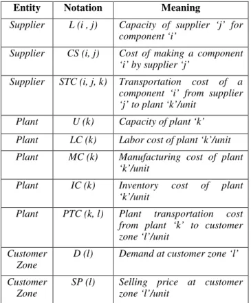
The following representation for data is used in this formulation. The data used in this model applies to suppliers, plants and customer zones. They can be fitted into two main categories i.e. costs and capacities. They are shown in Table 2.
Table 2: Notation For Data
2.2.3 Variables
There are three kinds of variables used in this formulation; they are vendor shipment variables, plant shipment variables and inventory variables. They are listed in Table 3. There are a total of 36 variables.
Table 3: Notation For Variables
Variable Meaning
Xi, j, k Amount of component ‘i’ from supplier ‘j’ to
plant ‘k’
Yk, l Amount of product shipped from plant ‘k’ to
customer zone ‘l’
Ii, k Inventory of component ‘i’ at plant ‘k’
2.3 PROBLEM FORMULATION
This section provides for a discussion of the inequalities (or equalities) and linear formulations depicting the constraints and objective functions respectively. These
Entity Notation Meaning
Supplier L (i , j) Capacity of supplier ‘j’ for
component ‘i’
Supplier CS (i, j) Cost of making a component
‘i’ by supplier ‘j’
Supplier STC (i, j, k) Transportation cost of a
component ‘i’ from supplier ‘j’ to plant ‘k’/unit
Plant U (k) Capacity of plant ‘k’
Plant LC (k) Labor cost of plant ‘k’/unit
Plant MC (k) Manufacturing cost of plant
‘k’/unit
Plant IC (k) Inventory cost of plant
‘k’/unit
Plant PTC (k, l) Plant transportation cost
from plant ‘k’ to customer zone ‘l’/unit
Customer
Zone D (l) Demand at customer zone ‘l’
Customer
formulations use four sets of two objective functions and different sets of constraints depending on which set of objective functions are used.
2.3.1 Constraints
The constraints listed below model the plant capacities, supplier capacities, inventory-balancing and total operating cost.
These six sets of equations depict the constraints used in the problem. Set of equations (1) and (2) depict plant and supplier capacity respectively. Set of equations (3), (4) and (5) depict inventory balancing constraints for components 1, 2 and 3 respectively. The last equation, (6) depicts the total operating cost (TOC) which is a sum of the transportation costs from suppliers to plants and plants to customer zones (TC), total manufacturing costs [TMC; which include the plant labor, inventory (IC) and manufacturing costs (MC)] and supplier costs (SC). Note that in the above constraints a variable S(i, j) is present. In a more generic formulation of this problem, S(i, j) would be a binary variable denoting whether component i can be supplied by supplier j or not. However, in this formulation, the S(i, j) values are fixed.
2.3.2 Objective Functions
Four sets of objective functions are used in this formulation are as follows:
Set 1:
Objective Function 1: Min TOC
Objective Function 2: Min MC/TOC
A justification for using these objective functions is as follows. Minimizing the total operating cost is an important performance metric in supply chain management problems. The second objective function denotes minimizing the ratio of manufacturing costs to total operating cost. We would like to ensure that our manufacturing costs fall within a certain permissible
bound as a percentage of the total operating cost. The decision maker based on his/her knowledge and expertise would be able to make an intelligible decision in choosing a solution.
Set 2:
Objective Function 1: Max Profit
Objective Function 2: Min MC
As can clearly be seen from Set 1 the two objective functions are conflicting because total operating cost features in the denominator in the second objective. In this set, the conflict is not so easily seen. The analysis will highlight the trade-off between the objectives.
Set 3:
Objective Function 1: Max Revenue
Objective Function 2: Min MC
In this set of objective functions the impact of the total operating cost is not taken into consideration. Only the revenue generated at the customer zones is considered. Its impact on the manufacturing costs is analyzed. In this set, the conflict in objectives cannot easily be seen from the equations that describe them. It is intuitive however that there will be conflict of interest when revenues and costs are studied.
Set 4:
Objective Function 1: Max Revenue
Objective Function 2: Min TC
This set of objectives is similar to that of set 3 except that here transportation costs are minimized, which feature as a necessary cost in every supply chain that has to be incurred in order to ensure interactions between the entities that make up the supply chain.
3
MULTI-OBJECTIVE
EVOLUTIONARY ALGORITHMS
Evolutionary algorithms are optimization algorithms that use the Darwinian theory of natural selection (Fogel, 1997, Darwin, 1859, ch. 6) as basis for optimization. Evolution, which is a result of natural selection, is an optimization method (Fogel, 1997, Mayr, 1988, p 104) which has had the luxury of having many years to complete its optimization or at least reach some kind of stable equilibrium. Evolutionary algorithms mimicking this behavior were first thought of for use in optimization by Prof. John H. Holland of The University of Michigan at Ann Arbor [for more information, see Holland, 1975]. There are many different types of evolutionary algorithms like genetic algorithms, evolutionary strategies (Rudolph, 1997), genetic programming and evolutionary programming (Porto, 1997). Genetic algorithms can also be combined with other artificial intelligence techniques like neural networks (Yao, 1999). Other examples of evolutionary algorithms include ant colony optimization
(
)
(
)
(
)
) 6 ( ) , ( ) ( ) ( ) ( ) , ( ) , , ( ) 5 ( ) 4 ( ) 3 ( ) 2 ( , ) , ( ) 1 ( , , , , , , , , 3 , , , 3 , 3 , 2 , , , 2 , 2 , 1 , , , 1 , 1 , , , , SC TMC TC TOC X S j i CS SC k IC k MC k LC TMC l k PTC Y k j i STC S X TC k I Y X S k I Y X S k I Y X S j i j i L X S k U Y i j k j i j i k k l kl i j k i jk i j k l kl j j jk k l kl j j jk k l kl j j jk k i j i j k k l l k + + = = + + = + = ∀ + = ∀ + = ∀ + = ∀ = ∀ ≤(Dorigo et al, 1996) and simulated annealing (Kirkpatrick et al, 1983) to mention a few.
In this application, evolutionary algorithms falling under the class of genetic algorithms (GAs) are used. Genetic algorithms (and similarly other evolutionary algorithms) are iterative and require a certain number of iterations (or
generations) to converge to the optimal solution. Genetic
algorithms work on the following principle:
1. Create a random population of n individuals 2. These solutions are then evaluated against a
fitness function
3. Create new members for the next population using the reproductive operators: crossover and
mutation
Fundamental to genetic algorithms are the three operators’ viz. selection, crossover and mutation. The crossover and mutation operators are diversity operators that bring diversity to the present population. Crossover is more explorative reproduction operator where traits from two individuals (parents) are combined to give traits for the new individual in the next generation (offspring or
children). Mutation is a less explorative and is performed on a single parent by mutating one or more parameters. Individuals that perform better when evaluated with the fitness function continue to the next generation and less fit individuals die out [natural selection, Darwin, 1859]. Genetic algorithms have traditionally been binary coded (handle binary representation of variables). However there are algorithms that can handle both real and binary coded variables. These traditional genetic algorithms could not handle multiple objectives and were meant to be used only for single objective optimization. Research in multi-objective genetic algorithms came about with the development of VEGA (Vector Evaluated Genetic Algorithm, Schaffer, 1984) and MOGA (Multi-Objective Genetic Algorithm, Fonseca and Fleming, 1993). Each of these algorithms suffered from their own setbacks. VEGA was a slight modification of traditional genetic algorithms and given m objectives, it randomly divides the population into m equal subpopulations. VEGA showed to be heavily biased toward one of the objectives functions in two-objective optimization problems. MOGA used stochastic universal selection, single point crossover and jump mutation. For fitness, MOGA used non-domination ranking and niching. It optimized the rank of the solution for lower rank. MOGA did not give robust results because it assigned ranks to individuals placed in non-dominated fronts (the front closest to the Pareto front) and higher ranks to those placed in fronts behind the 1st front. Since it
essentially optimized ranks, individuals in later fronts eventually died out. This proved to be a potential problem for the rest of the analysis, because individuals in later fronts might be having information that can eventually help the algorithm find all the solutions in the Pareto Non-Dominated front.
Srinivas and Deb, 1994 presented NSGA (Non-dominated Sorting Genetic Algorithm) which was based exactly on
MOGA except for a few changes in fitness assignment leaving the rest of MOGA unchanged. NSGA uses fitness sharing and ranking. It also ensures that all solutions placed in fronts closest to the non-dominated front will have higher fitness values than solutions placed in later fronts. When using a niching method such as fitness sharing it is essential to define a value, share which is a
distance metric. If the distance between two individuals is greater than or equal to share the individuals do not affect
each other’s fitness (Mahfoud, 1997). NSGA also implements the O(MN2) non-dominated sorting algorithm.
Thus for M objectives, one would need at the most O(N2)
comparisons where N is the population size. NSGA was able to deliver very good results and found solutions that almost completely filled the true Pareto front when evaluated with test functions. But disadvantages with NSGA lied with the specification of share, and that
stochastic universal selection is a non-elitist selection method which does not provide for sufficient selection pressure.
This paper utilizes the NSGA-II (Deb et al, 2002). NSGA-II uses a completely different methodology and implementation as compared to NSGA. NSGA-II implements elitism and crowded tournament selection. Elitism is a mechanism that ensures the best-fit individuals in a population are retained and thus one can be assured that good fitness obtained does not get lost in subsequent generations. Crowded tournament selection is a selection mechanism based on tournament selection whereby, a group of individuals takes part in a tournament and the winner is judged by the fitness levels (a combination of rank and crowding distance) that each individual brings to the tournament (Blickle, 1997). As noted by the authors, NSGA-II (Deb et al, 2002) handles the problems faced by earlier implementations of multi-objective evolutionary algorithms by incorporating elitism, using O(MN2) non-domination sorting complexity
and eliminating the need for specifying share.
A brief explanation of the steps involved in NSGA-II is presented below:
1. A parent population called Pt is randomly
generated and an offspring population Qt is
created from it.
2. Both populations Pt and Qt and combined into
population of size 2N where N is the population size. This new population is called Rt.
3. The population Rt undergoes non-dominated
sorting where all members are classified and put into fronts.
4. The best N individuals from Rt are selected using
the crowding tournament selection operator and from the parent population of the next generation
Pt+1.
5. The steps 1-4 are repeated until the termination criteria have been satisfied.
A typical mathematical formulation of a multi-objective optimization problem is as follows:
As can be seen, the formulation presented in section 2.3 agrees with the general template of equations (7) presented.
The source code for NSGA-II is freely available for research purposes at the KanGal (Kanpur Genetic Algorithms Laboratory) website. The website is maintained by Dr. Kalyanmoy Deb and is a portal to his continuing research in GAs. The code is implemented in the C programming language. The motivation for using NSGA-II in this paper is because it’s performance has been tested on several test functions and has given accurate results in generating the Pareto front as can be seen in Deb et al, 2002 and it is well supported by literature having been used in many real-world applications.
4
IMPLEMENTATION AND RESULTS
4.1 NSGA-II PARAMETER SETTINGS
In Reed et al, 2000, a Three-Step Design Methodology is presented which helps to specify the parameters required by NSGA-II (Deb et al, 2002). These parameters are:
1. Population size 2. Crossover probability 3. Mutation probability 4. Number of generations
For this paper, the crossover probability was set to 0.9 to allow for good explorative ability for the algorithm. The writers of NSGA-II suggest a range between 0.5 and 1.0 for crossover probability. All the variables are real-coded and the code-writers suggest a mutation probability between 0 and (no. of variables)-1 [0.278]. To balance the
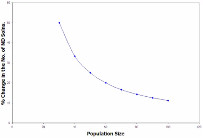
heavy exploration of crossover, the mutation probability was set to 0.01. The suggestions provided in Reed et al, 2000 for setting the population size are used. A small initial population size is used in the beginning and the population size is increased where at each step the percentage increase in the number of non-dominated solutions with respect to the previous step is noted. If this percentage increase falls below a certain pre-specified amount, then further increase in population size is not necessary. The formula used is as follows:
Where, ND is the pre-specified limit for percentage
increase, K is the number of non-dominated solutions obtained in the run i+1 and A is the number of non-dominated solutions obtained in the run i. The results for this preliminary analysis are shown in Figure 2.
Figure 2 illustrates the finding that the percentage increase in the number of non-dominated solutions decreases with an increase in the population size. It was observed that beyond a population size of 100, the percentage increase in the number of non-dominated solutions was too low. Thus, it would not justify the overhead of additional computational complexity that would be incurred if a higher population size were to be chosen. Therefore a population size of 100 was chosen for all the analyses that follow this discussion.
Figure 2: Change in the number of non-dominated solutions vs. population size.
In the subsequent section the results for the optimization are presented for the two sets of objective functions. The population size used is 100 and the change in the Pareto front is evaluated for number of generations: 250, 500, 700 and 1000.
4.2 RESULTS
NSGA-II gave good results and provided for a well populated Pareto front which a decision maker can use in making his/her analysis in choosing the solution that best embodies his/her intrinsic value for each objective. The results are presented for generation sizes of 500 and 700 only. For objective functions Set 1 the results are presented in Figures 3 and 4 for generations of 500 and 700 respectively. For objective functions Set 2 the results are presented in Figures 5 and 6 for generations of 500 and 500 respectively. The results for objective functions
Set 3 are presented in Figures 7 and 8 for generations of 500 and 700 respectively and for objective functions Set 4
in Figures 9 and 10, also for generations of 500 and 700 respectively.
{
}
n
i
x
X
x
K
k
x
h
J
j
x
g
to
subject
x
f
x
f
x
f
x
f
x
F
Min
u i i l i k j m,...,
2
,
1
,...,
2
,
1
,
0
)
(
)
7
(
,...,
2
,
1
,
0
)
(
;
)
(
),...
(
),
(
),
(
)
(
) ( ) ( 3 2 1=
≤
≤
=
=
=
≥
=
100
|
|
−
×
<
∆
A
A
K
NDFigure 3: Trade-off between TOC and MC/TOC for Population Size = 100 & Number of Generations = 500
Figure 4: Trade-off between TOC and MC/TOC for Population Size = 100 & Number of Generations = 700 As is illustrated from Figures 3 and 4, the Pareto front of efficient solutions is well populated for both generation sizes and the total operating cost (TOC) seems to vary between the values of 80,000 and 130,000 while the ratio of MC/TOC varies between the ranges of 0.3 to 0.45. The results presented here are for a single random seed. It can also be seen from Figures 3 and 4 that increasing TOC causes a decrease in MC/TOC. There is a clear trade-off in this set of objective functions. The decision maker can thus use intelligible decision making based on expertise to evaluate the Pareto front and choose those solutions that would be most beneficial to the system from a systems optimization perspective.
In general when a clear-cut decision cannot be made as to which solution is to be chosen, that solution which is closest (in terms of a pre-specified distance metric) to the extremum point which in this case would be the origin can be chosen as a candidate solution. This point (the origin) can be used as a reference point to evaluate the
solutions presented on the Pareto optimal front. The decision maker can then evaluate the performance of this solution on the entire supply chain and then choose to accept or reject the solution for a better one.
Figure 5: Trade-off between Profit and MC for Population Size = 100 & Number of Generations = 500
Figure 6: Trade-off between Profit and MC for Population Size = 100 & Number of Generations = 700
Figures 5 and 6 illustrate that the Pareto front of efficient solutions is well populated for both generation sizes and the values for profit vary between the 76,000 and 271,000 while the values for manufacturing cost (MC) vary between 43,7000 and 132,000. The results presented here are also for a single random seed. It can also be seen from Figures 5 and 6 that increasing Profit causes a subsequent increase in MC. There results also show a clear trade-off in the given set of objective functions.
In this case, the extremum point for the trade-off between a maximization-minimization problem would be the extreme point that gives the maximum profit and the minimum manufacturing cost. This is also a reference point that can be used for comparison when evaluating solutions.
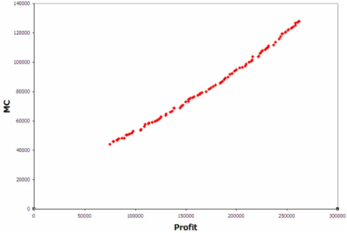
Figure 7: Trade-off between Revenue and Manufacturing Cost for Population Size = 100 & Number of Generations = 500
Figure 8: Trade-off between Revenue and Manufacturing Cost for Population Size = 100 & Number of Generations = 700
Figure 9: Trade-off between Revenue and Manufacturing Cost for Population Size = 100 & Number of Generations = 500
Figures 7 and 8 present the trade-offs between revenue and manufacturing cost for a single random number seed. The Pareto front shows an almost linear profile, but the results indicate a clear trade-off between the two objectives where maximization of revenue gives a high manufacturing cost.
Figure 10: Trade-off between Revenue and Manufacturing Cost for Population Size = 100 & Number of Generations = 700
Figures 9 and 10 illustrate the trade-offs between revenue and transportation costs for a single random number seed. The results show that higher numbers of generations do not necessarily lead to more populated Pareto fronts in the case of some objective function combinations as is clear from Figure 10. However the results do indicate a clear trade-off between the two objective functions.
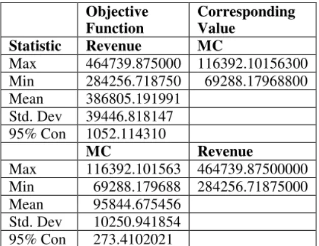
4.3 PERFORMANCE
A random seed analysis was performed for both sets of objective functions to obtain an idea about the stochastic nature of the results obtained through evolutionary computation. The runs were performed for a generation size of 500 and population size of 100 with other parameter settings remaining unchanged. The data is presented in Table 4 for Set 1 and in Table 5 for Set 2. The total number of random seeds in both analyses was 51. The results for Set 3 are presented in Table 6 and that for Set 4 in Table 7. A total of 54 random number seeds were used for the random seed analysis for Set 3 and 51 random seeds were used for the analyses for Set 4. The random seeds were generated by a random number generator written in the C programming language and fed to NSGA-II one at a time to obtain the results.
The results for performance include the maximum and minimum values of the objective functions over all values of random seeds and the corresponding values for the other objective at those maxima and minima. The results also contain values for the mean, standard deviation and the 95% confidence interval for each objective function set. The results provide for a synopsis of the random seed
analysis and also contain a range for each objective fucntion.
Table 4: Random Seed Analysis for Objective Function Set 1
Objective
Function Corresponding Value
Statistic TOC MC/TOC
Max 175129.609375 0.327840 Min 51477.074219 0.384800 Mean 107536.784915 Std. Dev 25380.061538 95% Con 701.175982 MC/TOC TOC Max 0.494218 111098.085938 Min 0.168562 87393.148438 Mean 0.356052 Std. Dev 0.051778 95% Con 0.004525
Table 5: Random Seed Analysis for Objective Function Set 2
Objective
Function Corresponding Value
Statistic Profit MC Max 280994.187500 129756.703125 Min 52039.582031 37570.750000 Mean 188021.082475 Std. Dev 45594.950157 95% Con 1260.279687 MC Profit Max 135679.109375 267313.718750 Min 35442.843750 53814.980469 Mean 87696.929625 Std. Dev 18810.017051 95% Con 519.9234197
Table 6: Random Seed Analysis for Objective Function Set 3
Objective
Function Corresponding Value Statistic Revenue MC Max 464739.875000 116392.10156300 Min 284256.718750 69288.17968800 Mean 386805.191991 Std. Dev 39446.818147 95% Con 1052.114310 MC Revenue Max 116392.101563 464739.87500000 Min 69288.179688 284256.71875000 Mean 95844.675456 Std. Dev 10250.941854 95% Con 273.4102021
Table 7: Random Seed Analysis for Objective Function Set 4
Objective
Function Corresponding Value
Statistic Revenue TC Max 497068.62500000 80233.38281300 Min 308609.46875000 47546.85546900 Mean 436037.48765828 Std. Dev 36426.07053919 95% Con 1032.84958016 TC Revenue Max 82803.61718800 493821.8750000 Min 47546.85546900 308609.4687500 Mean 66736.92726940 Std. Dev 6267.46296005 95% Con 177.71190774
5
CONCLUSIONS
This paper presents results for a hypothetical but realistic supply chain optimization problem. As can clearly seen by figures, NSGA-II provides a Pareto frontier of efficient solutions and these solutions can be used by the decision maker to design the supply chain. Tables 4 through 7 give a clear indication of the stochasticity involved. The potential to solve highly combinatorial problems using evolutionary algorithms is very large. Genetic algorithms have been under-utilized in this respect and hopefully, this paper illustrates that multi-objective evolutionary algorithms can be used to successfully model a supply chain.
Notations
MC : Manufacturing Cost
TC : Transportation Cost
TOC : Total Operating Cost
6
FUTURE WORK
The work elaborated in this paper is essentially work-in- progress and is ongoing. Future research initiatives include;
1. Modeling the entities in the supply chain as agents. In this approach, the entities would be independent autonomous agents each trying to maximize its own set of objective functions by playing non-zero sum games. Non-zero sum games can be used to incorporate co-ordination. In such games one player’s winnings does not necessarily have to come at the other player’s complete expense. In a two-player game, they can both gain by learning the set of parameters that will cause this co-ordination. Genetic algorithms would be well suited for such a combinatorial problem.
2. Introducing a stochastic demand at each node (for each entity). In real-life scenarios, demand is more or less stochastic with a seasonal nature that encompasses it. Forecasting and other prediction methods can only help to estimate what demand might be like in a particular quarter, month or week. For robustness to be incorporated in a supply chain model, stochasticity of demand is an important characteristic that needs to be implemented. With both these characteristics implemented, multi-objective system optimization of the supply chain is a challenging and interesting initiative. It would be apt to realize results which are similar to those elaborated in this work which would enable the decision maker is making even better choices of solutions.
Acknowledgments
I wish to thank Dr. Patrick Reed (Department of Civil and Environmental Engineering, Pennsylvania State University) and Dr. Soundar Kumara (Department of Industrial and Manufacturing Engineering, Pennsylvania State University) for their guidance throughout this project. I look forward to their support as I continue my efforts in taking this project to the next level. I also wish to acknowledge Venkat Devireddy for some good discussions.
References
L. Alwan, J. Liu and D-Q. Yao (2003). “Stochastic characterization of upstream demand processes in a supply chain,” IIE Transactions, Vol. 35, 207-219. B.C. Arntzen, G.G. Brown, T. P. Harrison and L. L. Trafton (1995). “Global Supply Chain Management at Digital Equipment Corporation,” INTERFACES, Vol. 25, pp. 69-93
J. Ashayeri and J. M. J. Rongen (1997). “Central Distribution in Europe: A Multi-Criteria Approach to Location Selection,” International Journal of Logistics
Management, Vol. 8(1), pp. 97-109
T. Blickle (1997). “Tournament Selection,” Handbook of
Evolutionary Computation, IOP Publishing Ltd and
Oxford University Press, pp. C2.3:1- C2.3:4
F. P. Buffa and W. M. Jackson (1983). “A Goal Programming Model for Purchase Planning,” Journal of Purchasing and Materials Management, Vol. 19 (3), pp 27-34
A. Cakravastia, I. S. Toha and N. Nakamura (2002). “A two-stage model for the design of supply chain networks,” International Journal of Production
Economics, Vol. 80, pp. 231-248.
M. A. Cohen and H. L. Lee (1988) “Strategic Analysis of Integrated Production-Distribution Systems: Models and Methods,” Operations Research, Vol. 36(2), pp. 216-228
C. R. Darwin (1859). “On the origin of Species by Means of Natural Selection or the Preservation of Favoured Races in the Struggle for Life,” London: Murray
K. Deb, A. Pratap, S. Agarwal and T. Meyarivan (2002). “A Fast and Elitist Multiobjective Genetic Algorithm: NSGA-II,” IEEE Transactions on Evolutionary
Computation, Vol. 6(2), pp. 182-197
M. Dorigo, V. Maniezzo and A. Colorni (1996). “The Ant System: Optimization by a colony of cooperating agents,”
IEEE Transactions on Systems, Man, and Cybernetics Part B: Cybernetics, 26(1), pp. 29-41
D. B. Fogel (1997). “Introduction,” Handbook of
Evolutionary Computation, IOP Publishing Ltd and
Oxford University Press, pp. A1.1:1- A1.1:2
C. M. Fonseca and P. J. Fleming (1993). “Genetic Algorithms for Multi-Objective Optimization: Formulation, Discussion and Generalization,”
Proceedings of the 5th International Conference on
Genetic Algorithms, pp. 416-423
I. Giannoccaro and P. Pontrandolfo (2002). “ Inventory management in supply chains: a reinforcement learning approach,” International Journal of Production
Economics, Vol. 78, pp. 153-161
D. A. Hicks (1999). “Four-step Methodology for using simulation and optimization technologies in strategic supply chain planning,” Proceedings of the 1999 Winter
Simulation Conference, Vol. 2 pp. 1215-1220.
J. H. Holland (1975). “Adaptation in Natural and Artificial Systems,” Ann Arbor, MI: University of Michigan Press
O. Jellouli and E. Chatelet. (2001). “Monte Carlo simulation and genetic algorithm for optimizing supply chain management in a stochastic environment, ” IEEE International Conference on Systems, Man and Cybernetics, Vol. 3 (7-10), Oct., pp. 1835-1839
J. Joines, M. A. Gokce, D. Gupta, R. King and M. Kay (2002). “Supply Chain Multi-Objective Simulation Optimization,” Proceedings of the 2002 Winter
Simulation Conference, pp. 1306-1314
S. Kirkpatrick, C. D. Gelatt, Jr., M. P. Vecchi (1983). “Optimization by Simulated Annealing,” Science, Vol. 220 (4598), pp. 671-680
S. M. Lee and L. J. Moore (1973). “Optimizing transportation problems with multiple conflicting objectives,” AIIE Transactions, Vol. 5 (4), pp.
R. R. Lummus, D. W. Krumwiede and R. J. Vokurka (2001). “The relationship of logistics to supply chain management: Developing a common industry definition,”
Industrial Management and Data Systems, Vol. 101 (8-9),
S. W. Mahfoud (1997). “Niching Methods,” Handbook of
Evolutionary Computation, IOP Publishing Ltd and
Oxford University Press, pp. C6.1:1- C6.1:4
E. Mayr (1988). “Toward a New Philosophy of Biology: Observations of an Evolutionist,” Cambridge, MA: Belknap
E. Melachrinoudis, and H. Min (2000). “The dynamic relocation and phase-out of a hybrid, two-echelon plant/warehousing facility: A multiple objective approach,” European Journal of Operations Research, Vol. 123, pp. 1-15
L. K. Nozick and M. A. Turnquist (2001). “Inventory, transportation, service quality and the location of distribution centers,” European Journal of Operations
Research, Vol. 129, pp. 362-371
V. W. Porto (1997). “Evolutionary Programming,”
Handbook of Evolutionary Computation, IOP Publishing
Ltd and Oxford University Press, pp. B1.4:1- B1.4:10 P. Reed, B. Minsker and D. Goldberg (2003). “Simplifying multiobjective optimization: An automated design methodology for the nondominated sorted genetic algorithm-II,” Water Resources Research, Vol. 39(7), pp. 1196- 2000.
G. Rudolph (1997). “Evolution Strategies,” Handbook of
Evolutionary Computation, IOP Publishing Ltd and
Oxford University Press, pp. B1.3:1- B1.3:6
J. D. Schaffer (1984). “Some Experiments in Machaine Learning Using Vector Evaluated Genetic Algorithms,”
PhD Thesis, Vanderbilt University, Nashville, TN
N. Srinivas, and K. Deb, (1995) “Multi-Objective function optimization using non-dominated sorting genetic algorithms,” Evolutionary Computation, Vol. 2, pp. 221-248
T. H. Truong and F. Azadivar (2003). “Simulation Based Optimization for Supply Chain Configuration Design,”
Proceedings of the 2003 Winter Simulation Conference, pp. 1268-1275.
C. Weber and J. Current (1993). “A Multi-Objective Approach to Vendor Selection,” European Journal of
Operations Research, Vol. 68, pp. 173-184
X. Yao, (1999). “Evolving Artificial Neural Networks”,