Lower bounds on the estimation performance in low complexity quantize and forward cooperative systems

(1)

R E S E A R C H

Open Access

Lower bounds on the estimation performance

in low complexity quantize-and-forward

cooperative systems

Iancu Avram

*

, Nico Aerts and Marc Moeneclaey

Abstract

Cooperative communication can effectively mitigate the effects of multipath propagation fading by using relay channels to provide spatial diversity. A relaying scheme suitable for half-duplex devices is the quantize-and-forward (QF) protocol, in which the information received from the source is quantized at the relay before being forwarded to the destination. In this contribution, the Cramer-Rao bound (CRB) is obtained for the case where all channel

parameters in a QF system are estimated at the destination. The CRB is a lower bound (LB) on the mean square estimation error (MSEE) of an unbiased estimate and can thus be used to benchmark practical estimation algorithms. Additionally, the modified Cramer-Rao bound (MCRB) is also presented, which is a looser but computationally less complex bound. An importance sampling technique is developed to speed up the computation of the MCRBs, and the MSEE performance of a practical estimation algorithm is compared with the (M)CRBs. We point out that the parameters of the source-destination and relay-destination channels can be accurately estimated but that inevitably the source-relay channel estimate is poor when the instantaneous SNR on the relay-destination channel is low; however, in this case, the decoder performance is not affected by the inaccurate source-relay channel estimate.

Keywords: Cooperative communication; Estimation; Cramer-Rao bound; Modified Cramer-Rao bound

1 Introduction

In wireless communication, multipath signal propaga-tion can cause destructive interference at the receiving antenna, giving rise to fading and limiting the maximum throughput of the system [1, 2]. This phenomenon can be combatted by introducing diversity into the system, such as frequency diversity provided by orthogonal frequency-division multiplexing (OFDM) [3] or spacial diversity pro-vided by multiple-input multiple-output (MIMO) systems [4, 5]. A novel means of providing diversity is cooperative communication, in which relays provide spatial diversity by creating multiple signal paths between the source and the destination [6]. Cooperative communication systems take advantage of the broadcast nature of the wireless medium. The information broadcast by the source termi-nal is received not only by the destination but also by other terminals nearby. Instead of ignoring this signal as is the

*Correspondence: [email protected]

Department of Telecommunications and Information Processing (TELIN, UGent), St-Pietersnieuwstraat 41, 9000 Ghent, BE, Belgium

case in a classical communication system, in a cooperative system, these nearby terminals act as relays, forwarding to the destination the information received from the source and thus creating additional signal paths [7, 8].

Different strategies can be used to implement the infor-mation forwarding, including amplify-and-forward (AF) [9], quantize-and-forward (QF) [10], decode-and-forward (DF) [11], and coded cooperation [12]. The AF protocol, in which the relay amplifies the signal received from the source before sending it to the destination, is well known for its seemingly low-complexity implementation. How-ever, when using half-duplex terminals which cannot send and receive data simultaneously, the information received from the source needs to be stored with high precision at the relay awaiting retransmission to the destination, requiring a large memory at the relay terminal. While this memory requirement might not be a concern for high-end mobile terminals, it can be of importance in low com-plexity applications such as sensor networks, where the sensor hardware complexity should be kept low in order to minimize production cost and to maximize battery life

(2)

[13]. In order to meet these complexity demands, the QF protocol has been introduced. In the QF protocol, the data received from the source is coarsely quantized at the relay before being stored into memory, requiring signifi-cantly less memory space as compared to the AF protocol. Despite its low complexity, it has been shown that the QF protocol can achieve a very satisfactory error performance that is very close to that of AF [10, 14].

The majority of the research on cooperative systems has been performed under the assumption of perfect channel state information (CSI). While this is useful for obtaining various information-theoretical results, the real-life situ-ation of imperfect CSI presents new challenges that need to be tackled. In contrast to a non-cooperative communi-cation system where only the source-destination channel needs to be estimated, cooperative communication sys-tems must also acquire the state of the source-relay and the relay-destination channels. Channel parameter esti-mation for QF has been discussed in [14, 15] for a protocol in which the relay estimates the source-relay (SR) chan-nel and forwards its estimate to the destination, while [16] describes a QF system in which all channel parameters are estimated at the destination. The latter system bene-fits from the decreased relay-side complexity. However, it poses a more complex estimation problem, as the source-relay channel is not directly observed by the destination. In order to tackle this estimation problem, in [16], the source-relay channel is abstracted to be a discrete chan-nel, characterized by a finite set of transition probabilities. In doing so, the estimation of the source-relay channel is greatly simplified, and the computational complexity at the destination is reduced. Furthermore, this makes the estimation of the estimation of the source-relay channel transition probabilities independent of the channel model and quantization method, making the results applicable to a large variety of systems.

Once an estimation algorithm has been obtained for a certain estimation problem, different approaches exist to benchmark the performance of the considered algo-rithm. A first approach is to compare the decoding error rate of a system in which the channel parameters are esti-mated to that of a system in which the channel parameters are considered to be known. The difference between the two error rates provides an indication about the perfor-mance of the estimation algorithm. A more fundamental way of studying the performance of an estimation algo-rithm is provided by the Cramer-Rao bound (CRB), which is a lower bound (LB) on the error variance of an unbi-ased estimate [17]; when an estimate exhibits an error variance that is close to the CRB, there is little room to improve the accuracy of the considered estimate. The opposite holds for an estimate having an error variance that is much higher as compared to the CRB. The CRB for the estimation of the channel parameters in a one-way

AF cooperative system using flat-fading channels has been obtained in [18], while in [19], the CRB is obtained for an AF and DF system in which multiple frequency offsets are considered. Lower bounds for the two-way relaying chan-nel, in which two terminals aided by a relay communicate with one another, have been obtained in [20–23] for the AF protocol.

In this contribution at hand, the (CRB) is obtained for a QF system in which all relevant channel parameters are jointly estimated at the destination. It is identified which channels are the most difficult to accurately estimate and to which degree the different channel estimates are cou-pled. By interpreting the cascade of the source-relay chan-nel and the quantization operation as a single discrete-input discrete-output channel, the results obtained in this contribution can be used to benchmark a wide variety of cases with minimal adjustments, such as a multi-hop QF relaying scheme often found in sensor networks. Because the CRB is difficult to evaluate in some cases, the modified Cramer-Rao bound (MCRB) is also considered, which has a lower complexity compared to the CRB and converges to the latter at high SNR [24, 25]. The MCRB for a sim-ilar system has been obtained in [26]. However, because the MCRB is not a tight bound at low SNR values, obtain-ing the value of the CRB is important in order to be able to benchmark the estimation performance over the com-plete SNR range. Moreover, the comparison between the CRB and MCRB also provides valuable insights.

The remainder of this contribution is organized as fol-lows. In Section 2, the system model is introduced. In Section 3, an expression is obtained for the CRB, where-after the MCRB is derived in Section 4. Next, in Section 5, the use of importance sampling (IS) is outlined, a tech-nique that can be used to drastically shorten numerical simulation times [28], without affecting the accuracy of the obtained bounds. Finally, numerical results are pre-sented in Section 6, whereafter conclusions are drawn in Section 7.

2 Channel model

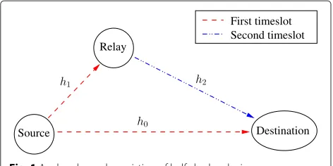
In this contribution, a cooperative network is analyzed consisting of a direct path and a one-hop relaying channel, as depicted in Fig. 1. The relay is considered to be a half-duplex device, meaning that it cannot send and receive information simultaneously. In a first frame, the source

broadcasts a sequence of K M1-PSK symbols, denoted

cs, which are received by both the relay and the destina-tion. The relay quantizes the angle of the received samples using log₂(M2) bits. These quantized samples,

repre-sented by a sequence ofK M2-PSK symbols denotedcr,

(3)

Fig. 1A relay channel consisting of half-duplex devices

2.1 Source-destination and relay-destination channels

The source-destination (SD) and relay-destination (RD) channels are modeled as flat Rayleigh fading channels with additive white Gaussian noise. The SD and RD channel coefficients are denotedh0andh2, respectively. The

sig-nals received by the destination from the source and the relay, denotedr0andr2, respectively, are equal to

r0=

Escsh0+n0

r2=

Ercrh2+n2.

(1)

Assuming the normalization |cs|2 = |cr|2 = K, the quantitiesEs and Er denote the transmitted energy per symbol at the source and the relay, respectively. The chan-nel coefficientsh0andh2are considered to be constant

during a frame and have a zero mean circular symmetric complex gaussian (ZMCSCG) distribution with variances Nh0 = 1/d0

nloss _and_N

h2 = 1/d2

nloss_{, respectively. The}

quantitiesd0 andd2 represent the distance between the

source and the destination and between the relay and the destination, whilenloss denotes the path loss exponent.

The components of the noise vectorsn0andn2are also

ZMCSCG distributed with respective variances N0 and

N2.

2.2 Equivalent source-relay channel

Due to the quantization operation, both the source and the relay transmit discrete symbols from a PSK constella-tion. Hence, the cascade of the source-relay (SR) channel and the quantization operation at the relay can be inter-preted as an equivalent discrete-input discrete-output

communication channel with M1 input values and M2

output values. Assuming that the actual SR channel and the quantizer are memoryless and time-invariant over a frame, this equivalent SR channel is fully characterized by M2×M1transition probabilitiesπq,m, which determine the probability of a symbol sent by the relay conditioned on the symbol sent by the source in the corresponding symbol interval, i.e., for q = 0,· · ·,M2 −1 and m =

0,· · ·,M1−1,

πq,m(k)=P

cr(k)=χM2(q)|cs(k)=χM1(m)

,

with χM(x) = e

j2πx

M _{. Denoting by} _r₁(_k) _the _k_th

sam-ple at the input of the relay, the transition probabilities

πq,m can be computed from the SR channel likelihoods pr1(k)|cs(k)=χM1(m)

and the quantization rule that mapsr1(k)toχM2(q). Results in this paper will be derived

in terms of the transition probabilities, without specify-ing the underlyspecify-ing SR channel likelihood and quantization rule.

It is further assumed thatM2/M1is integer and that the

quantization operation exhibits circular symmetry with respect to the symbols sent by the source, so that

π_q₊M₂

M₁m,m=πq,0=τq. (2)

Hence, the equivalent SR channel is characterized by the transition probabilities{τq,q=0,· · ·,M2−1}.

3 The Cramer-Rao bound

The CRB is a lower bound (LB) on the mean square error (MSE) of an unbiased estimate. In the current system model, the SD and RD channel coefficients,h0andh2, as

well as the SR transition probabilitiesτqare unknown and need to be estimated before the information transmitted by the source can be reliably detected at the destination. In order to keep the complexity of the relay terminal low, it is imposed that all parameters are estimated at the desti-nation. It is further assumed that the destination does not posses any a priori information on the different channel parameters.

The unknown channel parameters are grouped into the real-valued vectorθ, which is given by

θ =R(h0),I(h0),τT,R(h2),I(h2)

T ,

withτ =(τ0,τ1,· · ·,τM2−2)T. Note thatτM2−1is not

con-tained inθ, because it is not an independent parameter (τM2−1=1−τ0−. . .−τM2−2). In order to obtain the CRB,

the Fisher information matrix (FIM)J(θ) is introduced, the elements of which are defined as [17]

J(θ)i,j =Er _∂θ∂_ilnp(r;θ)_∂θ∂_j lnp(r;θ)

, (3)

with r = (r0,r2). It is shown in Appendix A that the

elements of the FIM can be expressed as

J(θ)i,j=Er

Xi(r;θ)Xj(r;θ)

, (4)

(4)

Er (θ−θˆ)(θ−θˆ)H

≥J−1(θ), (5)

whereA ≥Bimplies thatA−Bis positive-semidefinite matrix. Using (5), a LB can be obtained on the mean square estimation error (MSEE) of the various channel parameters as is shown in the next subsections. Note that the value of this LB depends on the specific realization of

θ. In order to obtain a LB that is independent of θ, the obtained expressions need to be averaged overθ, as will be done numerically in Section 6.

3.1 SD and RD channel coefficients

Once the elements of the FIM have been calculated, a LB on the MSEE of the SD and RD channel coefficients is obtained by noting that h0 and h2 can be expressed in

terms ofθash0=uθandh2=wθ, withu=(1,j,0M2+1)

andw=(0M2+1, 1,j), wherej2= −1. This yields the

fol-lowing CRB on the MSE arising from the estimation of h0:

Er |h0− ˆh0|2

≥uJ−1(θ)uH=CRBh0(θ). (6)

The CRB on the MSE arising from the estimation ofh2

is obtained by substitutinguforwin (6).

3.2 SR transition probabilities

Considering thatτ =Vθ with

the CRB on the MSE arising from the estimation ofτ is given by

3.3 Known parameter subset

It will be useful to also consider the CRB related to the estimation of a parameter subset {θi,i ∈ C} under the assumption that the complementary parameter set{θj,j∈

˜

C} is known, in order to evaluate the impact, on the

estimation of the former subset, of whether or not the lat-ter subset is known. The corresponding FIM is obtained by removing from the original FIM thejth rows andjth columns that correspond toj ∈ ˜C, leaving only the rows and columns that correspond to the unknown parameters {θi,i∈C}.

4 The modified Cramer-Rao bound

As shown in Appendix A, the calculation of the elements of the FIM involves the computation of the a posteriori probabilities of the source symbols, making it difficult to obtain a closed-form expression for the CRB. Therefore, when using non-trivial channel codes, the CRB needs to

be obtained using numerical simulations methods (see Section 5) that are quite time-consuming. In order to avoid the computational complexity associated with the CRB, we also consider the modified CRB (MCRB), which does not need the a posteriori probabilities of the source symbols (the MCRB assumes the source symbols are known by the receiver). The MCRB is a looser bound com-pared to the CRB; the CRB approaches the MCRB at high signal to noise ratios, wherep(cs(k)|r,θ) ≈ 1 for cs(k) equal to the symbol actually transmitted. Due to the less complex mathematics of the MCRB, simulation times are greatly reduced and in some cases closed-formed expres-sions can be found. The MCRB is obtained by substituting in (6) and (7) the inverse of the FIM with the inverse of the modified Fisher information matrix (MFIM), defined as [25]

It follows from (2) that

p(r(k)|cs(k)=χM1(m);θ)r(k)=y

=p(r(k)|cs(k)=χM1(0);θ)r(k)=yχM∗₁(m),

so that in (8) the conditional expectationEr|cs[ .] does not

depend on the particular realization ofcs. Hence, the outer expectation in (8) can be omitted, yielding

JM(θ)i,j=Er|cs

As shown in Appendix B,JMis a block-diagonal matrix equal to

related to the estimation of the SD channel parameters {θ0,θ1} and the source-relay-destination (SRD) channel

parametersθ¯ = {θi,i > 1}, respectively. It is shown in Appendix B that the elements ofJM,SRDcan be expressed

as components ofJM,SRDis given in (37) and (38). Because of

(5)

4.1 SD channel

Given the value ofJM,SD, the MCRB corresponding to the

estimation of the SD channel coefficienth0becomes

E | ˆh0−h0|2

of the SRD channel, the expectation in (10) must be com-puted using Monte-Carlo (MC) methods (see Section 5). However, in a few special cases considered below, closed-form expressions can be obtained.

4.2.1 Perfect RD channel

When the RD channel is perfect, the destination receives the message from the relay unaltered, i.e., r2 = cr. In this case, the estimation of the SRD channel parame-ters reduces to the estimation of the transition proba-bilities of the equivalent SR channel. Introducing θ˜ =

τ0,τ1,. . .,τM2−2

T

, the resulting FIM has dimension

(M2−1)×(M2−1), and is equal to

Using (37), (11) can be written as

JM,SR(θ˜)i,j=K

whereδxdenotes the Kronecker delta function. Hence, the MFIM can be represented as:

JM,SR(θ˜)=K

D−1+τ_M−1₂₋₁1T_M₂₋₁1M2−1

,

withDa diagonal matrix with diagonal elements equal to

(τ0,τ1,. . .,τM2−2). Using the Woodbury matrix identity

[27] to calculate the inverse of the MFIM yields

J−_M1_,SR(θ˜)= 1

The MCRB corresponding to the estimation of τ

is obtained by substituting (13) into (7) with V =

4.2.2 Perfect equivalent SR channel

When the equivalent SR channel is perfect, a symbol transmitted by the relay is completely determined by the corresponding symbol transmitted by the source; stated differently, all but one transition probabilities are zero, and the nonzero transition probability equals one. In this case,

the estimation of the SRD parameters reduces to the esti-mation of the RD channel coefficienth2. It can be shown

that one obtainsJM,RD=

2KEr

N2

I2, and subsequently

E | ˆhd−hd|2

In general, the evaluation of the FIM (4) and the MFIM (9) involves expectations that cannot be obtained in closed form, so that we must resort to MC techniques. However, when some of the transition probabilities of the SR chan-nel are very small, the computational effort required to obtain an accurate value for the (M)CRB can be very high. This can be understood by calculating the MCRB corre-sponding to the case of a perfect RD channel and using a MC approach instead of an analytical one. A straight-forward MC approach to obtainJM,SR(θ˜)i,j involves the following approximation of (12):

J_M_{, SR}(θ)˜ i,j≈ K arbitrary symbol from theM1-PSK constellation (say,cs= 1), and

c(n)r ,n=1, 2,. . .,N

is a sequence of i.i.d random

variables, generated according to Pr estimate (16) of the MFIM is singular (it has identicali1th

andi2th rows), so that its inverse does not exist. Hence,

to obtain meaningful results using (16), very large values of N (and, therefore, long simulation times) are required when some of the transition probabilities are very small.

These simulation times can significantly be shortened by the use of importance sampling (IS) [28]. For the exam-ple of the perfect RD channel, this involves generating

c(n)r ,n=1, 2,. . .,N

according to a biased distribution

(6)

for allq, so that (17) is close to the analytical result (12). By using IS, we have thus

In the general case,J(θ)i,jfrom (3) andJM,SRD(θ¯)i,jfrom (10) are approximated as

J(θ)i,j≈ 1 N

N

n=1

Xi

r(n);θ

Xj

r(n);θ

.p

r(n);θ pr(n);ζ

(18)

JM,SRD(θ¯)i,j≈ K N

N

n=1 ¯

Xir₂(n),cs;θ¯Xj¯ r₂(n),cs;θ¯.

pr(₂n)|cs;θ

pr(₂n)|cs;η ,

(19)

where r(n),n=1, 2,. . .,N! and

r(n)₂ ,n=1, 2,. . .,N

are N independent realizations generated according to the biased distributionspr(n);ζandp

r₂(n)|cs;η

, with

ζ =(R(h0),I(h0),κ0,κ1,. . .,κM2−2,R(h2),I(h2))T η=(κ0,κ1,. . .,κM2−2,R(h2),I(h2))T.

Note that the expression (18) of the FIM is much more time-consuming to evaluate than the expression (19) of the MFIM; indeed, the former requires the generation

of observation vectors of K components and the

com-putation of the a posteriori source symbol probabilities, whereas for the latter the observations to be generated are scalar, and no a posteriori source symbol probabilities are needed.

6 Numerical results

In this section, the value of the CRBs and MCRBs related to the various channel parameters is obtained for different SNRs. The IS technique from Section 5 has been applied to evaluate the MCRBs. No IS is used when computing the CRBs, due to the complexity involved in evaluating the factorpr(n);θ "pr(n);ζin (18).

In this section, the value of the CRB and MCRB is obtained for different SNR ratios using the IS technique from Section 5. First, the simulation parameters are spec-ified, whereafter the LBs on the MSEE of the different channel parameters are discussed. The tightness of the obtained LBs is evaluated by comparing the latter with the MSEE of the estimation algorithms from [16], which are briefly discussed in Appendix C.

6.1 System parameters

The SD and RD channels are as described in Section 2.1. The actual SR channel is modeled as a flat Rayleigh fading channel with additive white Gaussian noise, char-acterized by the channel coefficient h1. The latter is

constant during a frame and has a ZMCSCG distribu-tion with varianceNh1 = 1/d1

nloss_{, with}_d

1the distance

between the source and the relay terminal. The noise on the SR channel also has a ZMCSCG distribution with varianceN1.

The instantaneous SNRs on the SD, SR, and RD chan-nels are γ0 = Es|h0|2/N0, γ1 = Es|h1|2/N1, andγ2 =

Er|h2|2/N2, respectively; the corresponding average SNRs

areEs/N0,Es/N1andEr/N2. The source, relay, and

desti-nation terminals are located at the vertices of an equilat-eral triangle with normalized edge length, i.e.,d0=d1 =

d2=1, yieldingE[|hn|2]=1 forn=0, 1, 2. All noise vari-ances are taken equal (i.e.,N0 = N1 = N2). The source

symbols and the relay symbols have the same energy (i.e., Es=Er).

The source broadcasts BPSK symbols (i.e.,M1=2). The

samples received by the relay are quantized to QPSK sym-bols (i.e.,M2= 4) without knowledge of the SR channel,

i.e.,cr(k)=ej π

20.5+π2arg(r1(k))_with_r₁(_k)_{denoting the}_k_th

sample received by the relay. The corresponding transition probabilities of the equivalent SR channel are obtained as function of the SR channel parameters h1 andEs/N1

using the techniques described in [10, 16]. For the calcu-lation of the CRB, channel encoding is performed using a

(1, 13/15)8RSCC turbo code [29] that is punctured to a

rate of 2/3. A frame contains 1024 information bits, which corresponds to 1536 data symbols after channel encoding and BPSK mapping. In addition to these BPSK data sym-bols, 12 pilot symbols are added to each frame, to help the destination to obtain estimates for the various chan-nel parameters; this yields a total frame size ofK = 1548 BPSK symbols.

The CRB for a given realization ofθ is obtained by per-forming the averaging in (4) by means of a MC simulation involving N = 5000 independent realizations ofr; this corresponds to the generation of 2K·N≈1.5·107_scalar

observations. Subsequently, 104realizations ofθ are used to average the CRB overθ.

The calculation of the MCRB for a given realization of

θ is performed using MC simulation with IS. The biased transition probabilitiesκto be used in (19) are generated by assuming thatγ1is always equal to 0 dB, irrespective of

the actual value ofγ1. In doing so, only 5000 realizations

of the scalar observationr2that corresponds tocs=1 are generated to compute the conditional average overr2in

(10). When compared to the 1.5·107iterations required for the CRB where no IS is used, IS reduces the simu-lation time by a factor of 3000. While the calcusimu-lation of the (M)CRB is typically not a time-critical application, the simulation time reduction can prove very valuable when prototyping a system, where the changes applied to it can be rapidly benchmarked by means of the MCRB. After averaging overr2, 104realizations ofθare used to average

(7)

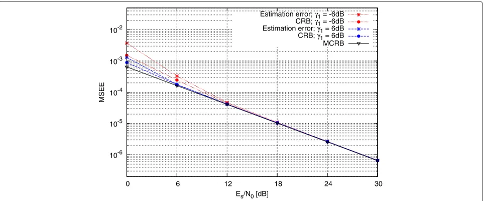
6.2 Estimation of the SD channel

The MSEE of the SD channel coefficient is analyzed as a function ofEs/N0, while keeping the instantaneous SNR

on the SR channel, represented byγ1, fixed. We setEr/N2

equal toEs/N0. Figure 2 shows the MSE resulting from

the EM algorithm, the CRB and the MCRB related to the estimation of h0 for various values ofγ1. The MCRB is

independent ofγ1, as was pointed out in Section 4.

How-ever, the CRB is affected by the value of γ1, because γ1

determines the transition probabilitiesτ, which in turn impact the a posteriori source symbol probabilities that are used in the computation of the CRB.

As the figure shows, the state of the SR channel, repre-sented byγ1, has only little impact on the MSEE of the

SD channel coefficient. As expected, this effect further diminishes at high SNRs, where the CRB approaches the MCRB.

6.3 Estimation of the SR channel

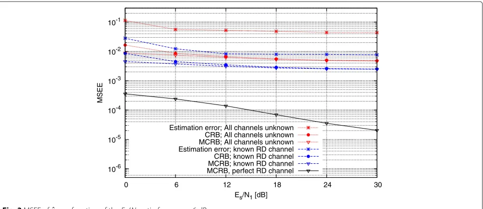
We consider the bounds on the MSEE of the equiva-lent SR channel transition probabilities τ, as a function of Es/N1, with the SD channel being characterized by

Es/N0 = Es/N1. We take fixed values forγ2, the

instan-taneous SNR of the RD channel. Figures 3, 4, and 5 show the CRB, the MCRB, and the MSEE resulting from the EM algorithm, for variousγ2. In order to evaluate the impact

of an imperfect RD channel estimatehˆ2on the estimation

performance of the SR channel transition probabilitiesτ, the aforementioned figures also show the results corre-sponding to the estimation ofτ whenh2is known to the

destination. As a LB on the obtained results, the MCRB corresponding to the case of a perfect RD channel (see Section 4.2.1) is also plotted.

Several key observations can be made from the afore-mentioned figures. At high γ2 values, shown in Fig. 5,

the CRB converges to the MCRB for moderate and highEs/N1when all channels are unknown and, at high

Es/N1, both the CRB and MCRB converge to the MCRB

corresponding to a perfect RD channel. Assuming the RD channel is known to the destination when estimat-ing, the SR channel yields only a slight decrease in

MSE. Figure 5 also shows that at high γ2 values, the

CRB is a tight LB on the MSE of the actual estimation algorithm.

For lowerγ2(see Figs. 3 and 4), the CRB still approaches

the MCRB at highEs/N1when all channels are unknown,

but there remains a substantial (especially at very low

γ2 values) gap in MSE as compared to the case where

the RD channel is known to the destination; a still larger gap occurs as compared to the case of a per-fect RD channel. The former gap is caused by the poor accuracy of hˆ2 at low γ2, which in turn deteriorates

the estimate of τ, even at large Es/N1; this indicates

a considerable coupling between the estimates hˆ2 and

ˆ

τ. The difference in MSE between the cases of known

RD channel and perfect RD channel is caused by the noise on the RD channel, and therefore increases with decreasingγ2.

Next, we observe a MSE floor that occurs at highEs/N1

whenγ2is low. This phenomenon is explained by

calcu-lating the MCRB corresponding to the estimation of the SR channel transition probabilities at the high SNR limit. For very highEs/N1, the transition probabilitiesτ satisfy τk ≈ 1 for a certain indexk= 0.5+(2/π)arg(h1)and τl ≈ 0 for l = k. Under this assumption, (37) can be written as

10-6 10-5 10-4 10-3 10-2

0 6 12 18 24 30

MSEE

Es/N0 [dB]

Estimation error; γ₁ = -6dB CRB; γ1 = -6dB

Estimation error; γ1 = 6dB

CRB; γ1 = 6dB

MCRB

(8)

10-6 10-5 10-4 10-3 10-2 10-1

0 6 12 18 24 30

MSEE

Es/N1 [dB]

Estimation error; All channels unknown CRB; All channels unknown MCRB; All channels unknown Estimation error; known RD channel CRB; known RD channel MCRB; known RD channel MCRB, perfect RD channel

Fig. 3MSEE ofτˆas a function of theEs/N1ratio forγ2= −6 dB

∂ ∂θ¯i

lnp(r2|cs;θ)¯ =

P r2cr=χM2

i+M2 M1m

;θ¯

−P r2cr=χM2

M2(M1+m) M1 −1

;θ¯

P rdcr=χM2

k+M2 M1m

;θ¯

.

(20)

Using (20) when evaluating (9) yields Fig. 6, in which the highEs/N1limit of the MCRB related to estimatingτ is

plotted as a function ofγ2. As the figure shows, the value

of the MSE floor observed on Figs. 3 and 4 is determined by the instantaneous RD channel quality γ2. The figure

also shows that this MSE floor drops very steeply when

γ2 > 0 dB, explaining the apparent absence of an MSE

floor on Fig. 5.

Figures 3, 4 and 5 indicate that the MSEE resulting from the EM algorithm does not approach the CRB at low val-ues ofγ2. This is due to the fact that the estimation scheme

described in [16] fails to obtain accurate estimates for the SR transition probabilities at low γ2, accounting for

the gap between the MSEE of the EM algorithm and the (M)CRB.

It should be noted that the inability to accurately esti-mate the SR transition probabilities at low γ2 has only

a minor effect on the error performance of the decoder at the destination, as observed in [16]. Indeed, at low

10-6 10-5 10-4 10-3 10-2

0 6 12 18 24 30

MSEE

Es/N1 [dB]

(9)

10-5 10-4 10-3

0 6 12 18 24 30

MSEE

Es/N1 [dB]

Fig. 5MSEE ofτˆas a function of theEs/N1ratio forγ2=6 dB

γ2, the decoder basically ignores the signal r2 received

from the relay and exploits only the SD signalr0; in this

case, the error performance of the decoder is essentially independent of the quality of the SR channel estimate.

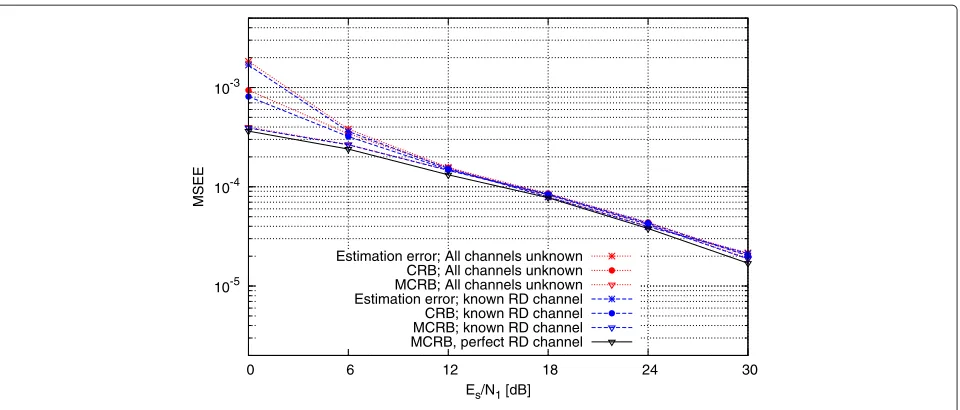
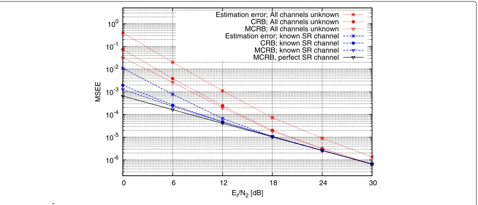
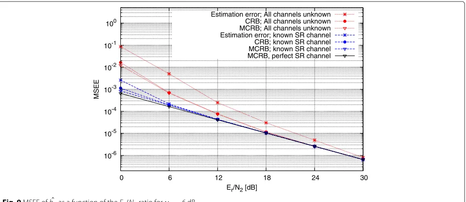
6.4 Estimation of the RD channel

The MSE resulting from the estimation of the RD chan-nel coefficient is shown in Figs. 7, 8 and 9 as a function of Er/N2. We takeEs/N0 = Er/N2, while keeping fixed

val-ues forγ1, the instantaneous SNR on the SR channel. As a

reference, the figures also show the results for a known SR channel (i.e.,τˆ=τ) and for a perfect SR channel (in which case the relay symbols are deterministically determined by the source symbols).

As the aforementioned figures show, the CRB converges to the MCRB at highEr/N2, and this irrespective ofγ1.

Unlike the LBs associated with the estimation of the SR channel transition probabilities, the CRB and MCRB of

the RD channel coefficient do not exhibit an MSE floor and, for anyγ1, both converge to the (M)CRB

correspond-ing to a known SR channel (τˆ =τ), and also to the MCRB corresponding to a perfect SR channel. This can be under-stood by consideringp(cr(k)|cs(k),r2(k);θ¯)from (38) for

very smallγ1, so thatτq≈ _M1₂,∀q; this yields

p(cr(k)|r2(k),cs(k);θ¯)=

p(r2(k)|cr(k);θ¯)

r2(k)p(r2(k)|cr(k);θ¯)

.

For largeEr/N2, we obtainp(cr(k)|cs(k),r2(k);θ¯) ≈ 1

whencr(k) equals the relay symbol actually transmitted. This indicates that, in spite of the very smallγ1, the relay

symbols can be considered known at the destination for largeEr/N2. This also enables the estimation algorithms

discussed in [16] to obtain accurate estimates ofh2,

mak-ing the CRB a tight LB on the estimation performance, especially so at high Er/N2 ratios. Hence, seen from an

10-30 10-25 10-20 10-15 10-10 10-5 100

-10 -6 -2 2 6 10 14

MSEE

γ2 [dB]

MCRB_τ at infinite SR channel SNR

(10)

10-6 10-5 10-4 10-3 10-2 10-1 100

0 6 12 18 24 30

MSEE

Er/N2 [dB]

Estimation error; All channels unknown CRB; All channels unknown MCRB; All channels unknown Estimation error; known SR channel CRB; known SR channel MCRB; known SR channel MCRB, perfect SR channel

Fig. 7MSEE ofhˆ2as a function of theEr/N2ratio forγ1= −6 dB

estimation point of view, it is advantageous to place the relay terminal close to the destination, as this enables the latter to obtain a good estimate of both the SR channel (due to a high averageγ2value) and the RD channel (due

to the robustness of the estimate ofh2with respect to low γ1values).

Comparison of the results obtained in this subsection to the bounds obtained for the SD channel in Subsection 6.2 indicates that due to the presence of the SR link, the RD channel is more difficult to accurately estimate. This effect diminishes as the SR channel quality is increased and especially if the SR channel is assumed to be known. In the case of a perfect SR channel, the MCRB related to the

estimation of the RD channel corresponds to that of the SD channel, as is to be expected.

7 Conclusions

In this contribution, the CRB was obtained for all chan-nels in a QF cooperative system. By maintaining a general description of the SR channel and the quantization opera-tion, the obtained results can be applied to a wide variety of cases such as a Rice fading SR channel or a cascade of different channels. In order to reduce the complexity asso-ciated with the CRB, we also presented the MCRB , which is a looser bound compared to the CRB but which con-verges to the latter at high SNR. Except for a few special

10-6 10-5 10-4 10-3 10-2 10-1 100

0 6 12 18 24 30

MSEE

Er/N2 [dB]

(11)

10-6 10-5 10-4 10-3 10-2 10-1 100

0 6 12 18 24 30

MSEE

Er/N2 [dB]

Fig. 9MSEE ofhˆ2as a function of theEr/N2ratio forγ1=6 dB

cases in which closed-formed expressions were found for the MCRB, the CRB and MCRB were obtained using numerical simulation methods. By using the proposed IS technique in the numerical computation of the MCRB, the simulation times were substantially reduced, allowing for fast benchmarking when making variations on a system under investigation.

The presented results show that it is possible to obtain accurate estimates of the SD and RD channels, irrespec-tive of the state of the other channels. On the other hand, accurately estimating the SR proves more difficult. The (M)CRB corresponding the estimation of the SR channel exhibits high MSEE values when the RD channel quality is poor. Furthermore, the MSEE of the SR channel param-eters is bounded by an error floor, the value of which depends on the state of the RD channel. Fortunately, the decoder performance is virtually unaffected by the accu-racy of the SR channel estimate when the RD channel quality is poor.

Notations a Scalar

a Column vector A Matrix

0N Row vector of lengthN with all elements equal to 0

1N Row vector of lengthN with all elements equal to 1

IN Identity matrix of rankN

(.)T,(.)H Transpose and Hermitian transpose Tr(.) Matrix trace

(.)∗ Complex conjugate |.| Absolute value

R(.),I(.) Real and imaginary part

Ex[ .] Expectation with respect to the random vectorx

Appendix A: Calculation of the FIM

In the following section, the calculation of the elements of the FIM is outlined. These elements are obtained by evaluating

J(θ)i,j=Er

_∂

∂θi

lnp(r;θ) ∂

∂θj

lnp(r2;θ)

=Er

Xi(r;θ)Xj(r;θ),

(21)

withXi(r;θ)= _∂θ∂_ilnp(r;θ). By conditioning on the sym-bolscsandcr sent by the source and the relay,Xican be written as

Xi(r;θ)= _∂θ∂ i

ln

cs,cr

p(r|cr,cs;θ)p(cr|cs;θ)p(cs)

=

cs,cr

F(r,cr,cs;θ)p(cr,cs|r;θ)

=Ecs,cr|r[F(r,cr,cs;θ)] ,

(22)

where

F(r,cr,cs;θ)= ∂

∂θi

lnp(r|cr,cs;θ)+ ∂

∂θi

lnp(cr|cs;θ).

Taking into account that

p(r|cr,cs;θ)=p(r0|cs;h0)p(r2|cr;h2)

(12)

Xi(r;θ)=

These expressions can be expanded as

Xi(r;θ)= (24) points in their respective constellations. In (25), the a posteriori probabilities p(cs(k)|r;θ) of the source sym-bols depend on the structure of the channel code, and are obtained from a soft decoder that operates onr. The joint a posteriori probabilitiesp(cs(k),cr(k)|r;θ)in (25) can be

The derivative in the first line of (25) reduces to

∂

and a similar expression holds for the derivative in the third line of (25). The derivative in the second line of (25) is expressed as

Based on the above expressions, the quantitiesXi(r;θ) can be evaluated for any (r,θ); the associated computa-tional complexity is rather high, because the calculation of

the a posteriori source symbol probabilitiesp(cs(k)|r;θ) requires a soft decoding operation.

Appendix B: Calculation of the MFIM

The elements of the MFIM are defined by (9) and are equal to

and the second term is zero fori≤1. Substituting (29) in (28) and evaluating the terms for whichθiis a parameter of the SD channel andθjis a parameter of the SRD channel (i.e.,i≤1,j>1) yields

so thatJM(θ)is a block-diagonal matrix which we repre-sent as

grouping the parameters from the SRD channel into the vectorθ¯= {θi,i>1}we obtain

where the summation overcr(k)runs over points of the M2-PSK constellation. Using (31), the elements ofJM,SRD

(13)

JM,SRD(θ¯)i,j=

Evaluation of the terms for whichk= ˜kyields

Er2|cs

Substituting (33), (34) into (32) yields

JM,SRD(θ)¯i,j=

for i > M2 −2. Having obtained closed-form

expres-sions forX¯i(r2,cs;θ¯), the expectation in (35) is evaluated by means of the importance sampling method outlined in Section 5.

Appendix C: Estimation of the unknown channel parameters

In order to evaluate the tightness of the obtained lower bounds, the latter are compared to the MSE results from the estimation algorithms described in [16], where maxi-mum likelihood (ML) pilot-based estimates of the various

channel parameters are refined using the expectation-maximization (EM) algorithm. In this section, we will briefly outline the estimation process. The reader is referred to [16] for further reading. When using the chan-nel model outlined in Section 6.1, the likelihood of the symbols received at the destination is equal to

p(r0,r2|cs,h0,h2,τ)

calculated in two steps. In a first step, pilot-based esti-mates of these parameters are obtained. To this purpose, Kppilot symbols are added to data symbols broadcast by the source in the first timeslot, resulting in frames consist-ing ofK+Kpsymbols. These pilot symbols are received by the destination, where they are used to calculate an estimate ofh0. They are also received by the relay, where

they are quantized together with the data symbols, and are broadcast to the destination in the second timeslot. The destination uses the pilot symbols received from relay to calculate an estimate ofτ andh2. Usingcspto denote the pilot symbols transmitted by the source, andr0pandr2pto denote the part ofr0andr2, respectively, that corresponds

to the received pilot symbols, the pilot-based ML esti-mates of the unknown channel parameters are obtained by solving the following equations:

ˆ

The first equation from (39) can be solved analytically, while the second is solved using the EM algorithm, where the quantized pilot symbols transmitted by the relay are considered to be nuisance parameters. The reader is referred to [16], section III-C, for a detailed resolution of (39).

After pilot-based estimates ofh0,h2andτare obtained,

they are refined using a code-aided EM approach. To this purpose, the data symbols transmitted by the source and the quantized symbols transmitted by the relay are con-sidered to be nuisance parameters. Each EM iterationi, refined estimates ofh0,h2andτ are obtained by solving

(14)

ˆ h0(

i)

,hˆ2(

i)

,τˆ(i)

=arg max

(h0,h2,τ) Q

h0,h2,τ,hˆ0(

i−1)

,hˆ2(

i−1)

,τˆ(i−1)

,

(40)

with

Qh0,h2,τ,hˆ0(

i−1) ,hˆ2(

i−1)

,τˆ(i−1)=Ecs,cr

lnp(r0,r2|cs,cr,h0,h2)+lnp(cr|cs,τ)r0,r2,hˆ0(

i−1) ,hˆ2(

i−1) ,τˆ(i−1)_.

The reader is referred to [16], section III-B, for the solution of (40). Using the results from [16], it can eas-ily be shown that the obtained estimates of h0, h2 and τ are unbiased, so that the CRB is indeed a LB for the considered estimates.

Competing interests

The authors declare that they have no competing interests.

Acknowledgements

The authors wish to acknowledge the Agency for Innovation by Science and Technology Flanders (IWT Belgium) that motivated this work. This research has been funded by the Interuniversity Attraction Poles Programme initiated by the Belgian Science Policy Office.

Received: 20 April 2015 Accepted: 6 October 2015

References

1. B Sklar, Rayleigh fading channels in mobile digital communication systems part I: characterization. IEEE Commun. Mag.35(7), 90–100 (1997) 2. TM Cover, JA Thomas,Elements of Information Theory. (Wiley, New York,

1991)

3. LJ Cimini Jr, Analysis and simulation of a digital mobile channel using orthogonal frequency-division multiplexing. EEE Trans. on Commun.33(7), 665–675 (1985)

4. GJ Foschini, MJ Gans, On limits of wireless communications in a fading environment when using multiple antennas. Wirel. Pers. Commun.6(3), 311–335 (1998)

5. G Foschini, Layered space time architecture for wireless communication in a fading environment when using multi-element antennas. Bell Labs. Tech. 1(2), 41–59 (1996)

6. A Sendonaris, E Erkip, B Aazhang, User cooperation diversity - part I:system Description. IEEE Trans. Commun.51(11), 1927–1938 (2003)

7. TM Cover, A El Gamal, Capacity theorems for the relay channel. IEEE Trans. Inf. Theory.25(5), 572–584 (1979)

8. A El Gamal, M Mohseni, S Zahedi, Bounds on capacity and minimum energy-per-bit for AWGN relay channels. IEEE Trans. Inf. Theory.52(4), 1545–1561 (2006)

9. JN Laneman,Cooperative Diversity in Wireless networks: Algorithms and Architectures. (Ph.D. dissertation, Massachusetts Institute of Technology, Cambridge, MA, 2002)

10. M Souryal, H You, inWCNC 2008. Quantize-and-Forward Relaying with M-ary Phase Shift Keying (IEEE Wireless Communications and Networking Conference Las Vegas, United, States, 31 Mar. –3 Apr 2008), pp. 42–47 11. JN Laneman, DNC Tse, GW Wornell, Cooperative diversity in wireless

networks: efficient protocols and outage behavior. IEEE Trans. Inf. Theory. 50(12), 3062–3080 (2004)

12. TE Hunter, S Sanayei, A Nosratinia, Outage analysis of coded cooperation. IEEE Trans. Inf. Theory.52(2), 375–391 (2006)

13. YW Hong, WJ Huang, FH Chiu, CCJ Kuo, Cooperative communications in resource-constrained wireless networks. IEEE Signal Process. Mag.24(3), 47–57 (2007)

14. I Avram, N Aerts, D Duyck, M Moeneclaey, A Novel Quantize-and-Forward Cooperative System: Channel Estimation and M-PSK Detection

Performance. EURASIP J. Wirel. Commun. Netw. Article, ID 415438, 11 pages (2010)

15. I Avram, N Aerts, M Moeneclaey,A Novel Quantize-and-Forward Cooperative System: Channel Parameter Estimation Techniques. (Future Network & Mobile Summit 2010, Florence, Italy, 16–18 Jun 2010) 16. I Avram, N Aerts, H Bruneel, M Moeneclaey, Quantize and forward

cooperative communication: channel parameter estimation. IEEE Trans. Wireless Commun.11(3), 1167–1179 (2012)

17. CR Rao, Information and the accuracy attainable in the estimation of statistical parameters. Bulletin of Cal. Math. Soc.37(3), 81–91 (1945) 18. S Zhang, F Gao, J Li, M Sheng, Online and offline Bayesian Cramer–Rao

bounds for time-varying channel estimation in one-way relay networks. IEEE Trans. Signal Process.63(8), 1977–1992 (2015)

19. H Mehrpouyan, SD Blostein, Bounds and algorithms for multiple frequency offset estimation in cooperative networks. IEEE Trans. Wireless Commun.10(4), 1300–1311 (2011)

20. Z Jiang, H Wang, Z Ding, A Bayesian algorithm for joint symbol timing synchronization and channel estimation in two-way relay networks. IEEE Trans. Wireless Commun.61(10), 4271–4283 (2013)

21. S Abdallah, IN Psaromiligkos, Partially-blind estimation of reciprocal channels for af two-way relay networks employing M-PSK modulation. IEEE Trans. Wireless Commun.11(5), 1649–1654 (2012)

22. S Abdallah, IN Psaromiligkos, Blind channel estimation for amplifyand-forward two-way relay networks employing M-PSK modulation. IEEE Trans. Signal Process.60(7), 3604–3615 (2012) 23. S Zhang, F Gao, C-X Pei, Optimal training design for individual channel

estimation in two-way relay networks. IEEE Trans. Signal Process.60(9), 4987–4991 (2012)

24. AD Andrea, U Mengali, R Reggiannini, The modified Cramer-Rao bound and its application to synchronization problems. IEEE Trans. Commun.42, 1391–1399 (1994)

25. M Moeneclaey, On the True and the modified Cramer-Rao bounds for the estimation of a scalar parameter in the presence of nuisance parameters. IEEE Trans. Commun.46(11), 1536–1544 (1998)

26. I Avram, M Moeneclaey, inWCNC 2013. The Modified Cramer-Rao Bound for Channel Estimation in Quantize-and-Forward Cooperative Systems (IEEE Wireless Communications and Networking Conference (WCNC) Shanghai, China, 7–10 Apr 2013), pp. 2862–2867

27. M Woodbury,Inverting modified matrices. (Memorandum Rept. 42, Statistical, Research Group, Princeton University, Princeton, NJ, 1950) 28. JM Hammersley, DC Handscomb,Monte Carlo Methods. (Methuen & Co.,

London, and John Wiley & Sons, New York, 1964)

29. S Lin, D Costello,Error Control Coding. (Pearson Education Inc., second edition, 2004)

Submit your manuscript to a

journal and beneﬁ t from:

7Convenient online submission 7Rigorous peer review

7Immediate publication on acceptance 7Open access: articles freely available online 7High visibility within the ﬁ eld

7Retaining the copyright to your article