10-8-2002
Bayesian Life Test Planning for the Weibull
Distribution with Given Shape Parameter
Yao Zhang
Iowa State University
William Q. Meeker
Iowa State University, [email protected]
Follow this and additional works at:http://lib.dr.iastate.edu/stat_las_preprints Part of theStatistics and Probability Commons
This Article is brought to you for free and open access by the Statistics at Iowa State University Digital Repository. It has been accepted for inclusion in Statistics Preprints by an authorized administrator of Iowa State University Digital Repository. For more information, please contact
Recommended Citation
Zhang, Yao and Meeker, William Q., "Bayesian Life Test Planning for the Weibull Distribution with Given Shape Parameter" (2002).
Statistics Preprints. 21.
Parameter
Abstract
This paper describes Bayesian methods for life test planning with Type II censored data from a Weibull distribution, when the Weibull shape parameter is given. We use conjugate prior distributions and criteria based on estimating a quantile of interest of the lifetime distribution. One criterion is based on a precision factor for a credibility interval for a distribution quantile and the other is based on the length of the credibility interval. We provide simple closed form expressions for the relationship between the needed number of failures and the precision criteria. Examples are used to illustrate the results.
Keywords
Bayesian design, Conjugate prior, Exponential distribution, Life data, Sample size determination
Disciplines
Statistics and Probability
Comments
This preprint was published inMetrika61 (2005): 237–249, doi:10.1007/s001840400334.
Distribution with Given Shape Parameter
Yao Zhang and William Q. Meeker
Department of Statistics
Iowa State University
Ames, IA 50011
October 8, 2002
Abstract
This paper describes Bayesian methods for life test planning with Type II censored data from a Weibull distribution, when the Weibull shape parameter is given. We use conjugate prior distributions and criteria based on estimating a quantile of interest of the lifetime distribution. One criterion is based on a precision factor for a credi-bility interval for a distribution quantile and the other is based on the length of the credibility interval. We provide simple closed form expressions for the relationship between the needed number of failures and the precision criteria. Examples are used to illustrate the results.
Key words: Bayesian design; Conjugate prior; Exponential distribution; Life data; Sample size determination.
1
Introduction
1.1
Problem
Life testing is an important method for evaluating component reliability. In applica-tions, a sample of units is tested under particular conditions to estimate the lifetime properties of the component at these conditions. Because of the often high reliability of the tested components and time/cost constraints of the experiment, life tests are usually terminated after a specific amount of time elapses (time or Type I censoring) or after a specific number of failures have been observed (failure or Type II censoring). Careful planning for how many units are to be tested and the length of the experiment (for Type II censoring, how many failures are to be observed) is important to obtain the maximum possible information with the minimum cost possible, on the average. Often the purpose of a life test is to estimate a specific quantile of the lifetime distribution, for instance, the 0.10 quantile. A life test can then be planned according to the needed estimation precision for this quantile. The Weibull and lognormal dis-tributions are appropriate to describe the variation in the lifetimes of many different types of components. In the traditional approach to the test planning problem, the goal is to estimate unknown fixed parameters and “planning values” of the distri-bution parameters are used for planning purposes (cf. Chapter 10 of Meeker and Escobar 1998). The Bayesian approach arises naturally when information is available a priorifor planning andestimation. This happens frequently in practical situations when there is available engineering or physical knowledge, or previous experience with similar components having the same failure mechanisms. Careful planning with rel-evant prior information can reduce needed experimental resources. For log-location-scale distributions such as the Weibull and lognormal distributions, Bayesian methods usually yield no closed forms for inferences on the planning criteria, partly because of the censoring. Numerical methods must be applied instead. For the Weibull distribu-tion with a given shape parameter, however, closed forms exist if standard conjugate
prior distributions are used. The given shape parameter Weibull cases are impor-tant in certain practical applications. Section 2.3 of Nordman and Meeker (2002) describe several applications where it is appropriate to use a given shape parameter. For example, the exponential Raleigh distributions are special cases when the Weibull shape parameter is given as one and two, respectively. Also, the planning solutions for these special cases provide useful insight into the more complicated planning prob-lem where the Weibull shape parameter is unknown. In this paper, we describe the Bayesian approach of life test planning for the Weibull distribution with given shape parameter, and provide the closed forms for the planning criteria. Planning solutions are illustrated with numerical examples.
1.2
Overview
The remainder of this paper is organized as follows.
• Section 2 reviews previously published related work.
• Section 3 describes the Bayesian planning problem for the Weibull distribution
with a given shape parameter, with a conjugate prior formulation.
• Section 4 presents numerical examples that illustrate the Bayesian planning
solutions and comparisons with results from the non-Bayesian approach. • Section 5 gives some concluding remarks and describes areas for future research.
2
Related Work
Numerous results for life test planning are available in the statistical and engineering literature. Many non-Bayesian approaches have been developed for different life test-ing considerations. Gupta (1962), Grubbs (1973), and Narula and Li (1975) describe sample size determination methods for controlling error probabilities in hypothe-sis testing of life distribution parameters and functions of distribution parameters.
Meeker and Nelson (1976) describe the asymptotic theory and application for plan-ning a life test to estimate a Weibull quantile with a specified precision. Meeker and Nelson (1977) also present general theory and application for approximate sample size determination in life test planning when other functions of Weibull parameters are to be estimated. Danziger (1970) describes life test planning for estimating the hazard rate of a Weibull distribution with a given shape parameter. Meeker, Escobar, and Hill (1992) present asymptotic theory and methods for planning a life test to estimate a Weibull hazard function, when all parameters are unknown .
Using prior information and Bayesian techniques in life test planning has also been explored in previous work. Thyregod (1975) develops an approximate method using Type II censoring with an exponential life distribution. His method uses a cost-based utility function and a Taylor expansion around the estimated mean to incorporate prior information. Zaher, Ismail, and Bahaa (1996) present Bayesian life test planning methods for the Weibull distribution with a known shape parameter under Type I censoring, using a criterion based on expected gain of Shannon information. The paper uses approximations and numerical solutions to obtain test plans.
More recently, there has been a series papers describing Bayesian theories, meth-ods, and discussions of the general sample size determination problem. For example, Joseph, Wolfson and Berger (1995a,b) provide three Bayes criteria based on highest posterior density (HPD) intervals for the sample size determination problem and il-lustrate the calculations for binomial proportions. These Bayesian approaches are based on the precision of interval estimation for a particular quantity of interest. Lindley (1997) provides a fully Bayesian treatment for the sample size problem based on a utility function, and compares the method with other Bayes criteria based on interval estimation precision, in particular, with the average length criterion (ALC) proposed by Joseph, Wolfson and Berger (1995a,b). Pham-Gia (1997) makes more comparisons between these two kinds of criteria, outlying the differences and simi-larities, and making an effort to better match them by using a utility function for
the ALC criterion. Joseph and Wolfson (1997) discuss the advantages and disadvan-tages of using these two kinds of criteria with an emphasis on the practical aspects. Bernardo (1997) illustrates the decision-theoretic Bayesian approach suggested by Lindley (1997) in the particular case where inference is seen as a decision problem with an action space consisting of the class of possible distributions of the relevant quantity and the utility function being a logarithmic score. Adcock (1997) argues that it is not always necessary to use the utility function in a Bayesian approach and, by example, shows, for some cases, the equivalence of the utility function and the average length Bayesian procedures.
3
Planning Problem
3.1
Model and Bayes Estimation
Suppose that the lifetimes of the units being tested have a Weibull(η, β) distribution with pdf f(t|η, β) = β η t η β−1 exp − t η β ,
whereηis the unknown scale parameter andβis the given shape parameter. Here we
consider the life test planning problem when the test is Type II censored with sample size n and fixed number of failuresr. The likelihood is
L(β, η;t) = β r ηr r 1t(i) ηr β−1 exp −T T Tβ ηβ , where t(i) is the ith ordered lifetime and
T T Tβ = n i=1 tβi = r i=1 tβ(i)+ (n−r)tβ(r)
is the “total transformed time on test” on the β-power scale.
Assume also that prior information on the scale parameter of the lifetime distri-bution is available. Letθ=ηβ denote the transformed scale parameter of the lifetime
model on theβ-power scale. An inverted gamma distribution IG(a, b) forθ provides a flexible conjugate prior representation for the prior information, and the prior density is ω(θ|a, b) = b a Γ(a)θa+1 exp −b θ , (1)
where the hyperparameters a > 0 and b > 0 are given. In practical applications
with informative prior information on the Weibull scale parameter η = θ1/β, the
prior variance is usually finite, which implies a > 2/β. In any case, the posterior distribution of θ is
f(θ|t, β, a, b) = ω(θ|a, b)×L(β, θ
1/β;t) ω(θ|a, b)×L(β, θ1/β;t) d(θ)
∼ IG(a+r, T T Tβ +b), (2)
which is also an inverted gamma distribution. Whena+r >2, the posterior variance is finite. This means that with a sufficient number of failures (r) the experiment will provide a posterior with finite variance, even in cases where prior variance does not exist (i.e., a ≤ 2/β). Bayes estimation of any function of the unknown parameter θ can be based on this posterior distribution of θ.
3.2
Planning Based on Precision of a Quantile
A commonly used reliability metric is the p quantile of the lifetime distribution,
tp = [−θlog(1−p)]1/β. (3)
We propose two ways of planning by considering the precision when using Bayes estimation of tp.
3.2.1 Criterion based on a large sample approximate posterior precision
factor (LSAPPF)
When using a large sample approximation (e.g., in more complicated problems for which closed-form solutions are not available), quantification of precision for
estimat-ing a positive quantity liketp is often performed in the log scale. In large samples, the posterior credibility interval fortp can be expressed, approximately, as [tp/R, tp×R], where tp is the Bayes estimate oftp and R is a posterior credibility interval precision factor
R = exp
z1−α/2
VarP osterior(logtp)
, (4)
and z1−α/2 is the 1−α/2 quantile of standard normal distribution. Here R serves as
a metric for estimation precision. From the posterior distribution of θ in (2), VarP osterior(logtp) = 1
β2VarP osterior(logθ)
= 1 β2VarP osterior log θ T T Tβ+b = 1 β2ψ (a+r), (5)
whereψ(z) =dψ(z)/dzis the polygamma function,ψ(z) = Γ(z)/Γ(z) is the digamma function, and Γ(z) is the gamma function. The justification of the last step in (5) is given in the Appendix. Combining (4) and (5) gives
R = exp z1−α/2 ψ(a+r) 1/β. (6)
Note that R depends only onα, r, β and the hyperparameter a but not on the data.
Thus R can be used as a criterion for test planning. Because it is the number of
failures r rather than the sample size n that affects the precision of estimation of tp, the number of failures can be chosen before the experiment to control the precision of estimation of thepquantile in terms ofR, as a function of the given prior information. The sample size ncan be chosen based upon time and cost availability considerations (with the constraint r ≤n), where the expected test length will be shorter for larger n. Also note that R does not depend on the value ofp, so that the planning solution is the same for all quantiles of the lifetime distribution.
3.2.2 Criterion based on an exact relative posterior credibility interval length (ERPCIL)
A Bayes credibility interval for tp that does not depend on the large sample
nor-mal approximation can be constructed directly from the posterior distribution. Let Lα(tp|t) denote the length of the 100(1−α)% credibility interval from the posterior distribution of tp. Then using the posterior distribution of θ in (2),
Lα(tp|t) = [−log(1−p)]1/βLα(θ1/β|t) = [−log(1−p)]1/β 1 qgamma1/β (α/2;a+r) (T T Tβ+b)1/β, (7) where 1 qgamma1/β (α/2;a+r) = 1 q1gamma/β (α/2;a+r) − 1 q1gamma/β (1−α/2;a+r),
and qgamma(α/2;a+r) is the α/2 quantile of gamma probability distribution with shape parameter (a+r) and unit scale parameter. This exact posterior credibility interval length depends on the data through T T Tβ, the value of p, and both prior hyperparameters a and b. Estimation precision of a positive quantity liketp is more reasonably specified relative to the value of tp to be estimated. Such a relative preci-sion metric is Lα(tp|t) E(tp|t) = Γ(a+r) Γ(a+r− β1) 1 qgamma1/β (α/2;a+r) , (8)
where E(tp|t) is evaluated relative to the posterior distribution of θ (2), based on the relationship (3) between tp and θ. Because the metric in (8) does not depend on the data, it can be used as a planning criterion. Planning solutions can be obtained according to the value of this criterion specified by the experimenter. Similar to
the LSAPPF criterion in (6), this criterion depends on the number of failures r,
rather than the sample sizen. Also, the planning solution does not depend onp, the particular quantile.
3.2.3 Exponential distribution case
The exponential distribution, as the special case of the Weibull distribution with given shape parameterβ = 1, has the following particular forms of the criteria in (6) and in (8).
• The LSAPPF criterion:
R = exp z1−α/2 ψ(a+r) . (9)
• The ERPCIL criterion:
Lα(tp|t) E(tp|t) = (a+r−1) 1 qgamma(α/2;a+r) , (10) where 1 qgamma(α/2;a+r) = 1 qgamma(α/2;a+r)− 1 qgamma(1−α/2;a+r).
4
Numerical Examples
This section uses numerical examples to illustrate the life test planning procedures obtained in the previous section. We also illustrate the correspondence of the Bayes test plans when prior information is vague to test plans from a non-Bayesian approach.
4.1
Setup
Suppose that an experimenter is interested in estimating a quantile of the lifetime distribution of a specific component, and that the estimation precision is to be based on a 95% credibility level (α= 0.05). Assume that the lifetimes of the component have
a Weibull distribution, and the shape parameter β of the distribution is given, but
that the scale parameterηis unknown. In addition, assume that prior information on the scale parameterη is available before the experiment, specified in terms of a prior
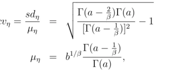
conjugate prior specification of θ = ηβ in (1), the relationships between the prior hyperparameters (a, b) andµη and sdη are
cvη = sdη µη = Γ(a− β2)Γ(a) [Γ(a−β1)]2 −1 (11) µη = b1/β Γ(a− 1β) Γ(a) , (12)
where cvη = sdη/µη is the coefficient of variation (CV) of the prior distribution for η. Note that the prior hyperparameter a is a function of the priorcvη (and the given Weibull shape parameterβ) only. In general, only numerical solutions ofa and b can be found, but for the exponential distribution (β = 1), these relationships reduce to
a = cvη−2+ 2 (13)
b = 1
µη(cvη−2+ 1).
For the Weibull distribution, Table 1 gives values of (a, b) for some combinations ofβ andcvη, whenµη = 1. Life test planning procedures presented in the previous section will be illustrated under these numerical conditions.
Table 1: Values of prior hyperparameters (a, b) when µη = 1
β = 0.5 β = 1 β = 2 β = 5 cvη a b a b a b a b 0.1 404.47 402.97 102 101 26.123 25.374 4.7011 4.1108 0.2 104.49 102.99 27 26 7.3676 6.6223 1.6532 1.0875 0.5 20.458 18.952 6 5 2.0876 1.3595 0.6865 0.2002 1.0 8.3723 6.8541 3 2 1.2945 0.5891 0.4898 0.0674 ∞ 4 2.4495 2 1 1 0.3183 0.4 0.0263
4.2
Planning with the LSAPPF Criterion
If the precision for estimation of tp is considered in terms of the precision factor R, the LSAPPF criterion in (6) can be used for the planning. Note that this criterion is not a function of the prior hyperparameter b, implying that the planning solution from this criterion is uniformly valid for any prior mean of η, as long as the prior hyperparameter a (or equivalently cvη) is specified [cf. (11) and (12)]. As previously
mentioned, neither does this criterion depend on the value of p of the quantile of
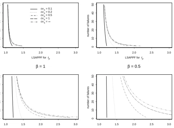
interest. Figure 1 gives the number of failuresras a function of the LSAPPF criterion value, for the different combinations ofcvη and β provided in Table 1.
Figure 1 shows that, for any given shape parameter, the necessary experimental resources (number of failuresr) increases, as expected, with larger required estimation precision. This increase in the necessary resources grows substantially when high estimation precision is required. On the other hand, needed experimental resources decreases with increasing prior information (decreasing prior CV). This is especially true when the prior CV on the scale parameter is small (e.g.,cvη <1). When the prior CV for the scale parameter is already large (cvη >1), further reduction in the amount of prior information results in only small increases in the number of failuresrrequired
and the increase is only noticeable for large values of R. This can be explained
intuitively by noting that prior information can be interpreted as prior “pseudo-samples,” and the prior CV is inversely proportional to the prior “pseudo-sample”
size [cf. expression (13) and the correspondence between the prior hyperparameter a
and number of failures r in criterion (6)]. When the prior cvη is greater than 1, the prior “pseudo-sample-size” falls to a small number and a large amount of change in specified precision implies only a small amount of change in required sample size. The information from the current experiment dominates, unless the current sample size is also small and little estimation precision is required. When the priorcvη decreases to a certain point, a substantially increased amount of prior “pseudo-data” is implied, and the needed experimental resources can therefore be reduced significantly.
1.0 1.5 2.0 2.5 3.0 LSAPPF for tp 0 1 02 0 3 04 0 5 0 number of failures β = 5 cvη = 0.1 cvη = 0.2 cvη = 0.5 cvη = 1 cvη = ∞ 1.0 1.5 2.0 2.5 3.0 LSAPPF for tp 0 1 02 0 3 04 0 5 0 number of failures β = 2 1.0 1.5 2.0 2.5 3.0 LSAPPF for tp 0 1 0 2 03 04 0 5 0 number of failures β = 1 1.0 1.5 2.0 2.5 3.0 LSAPPF for tp 0 1 0 2 03 04 0 5 0 number of failures β = 0.5
Figure 1: Needed number of failures as a function of LSAPPF fortp, when the Weibull shape parameter β is given and α= 0.05.
Figure 1 also shows the effect of different given values of the Weibull shape param-eterβ. For a certain specified precision R, small values ofβrequire more experimental
resources. This is because Weibull distributions with smaller values of β have more
relative variability. Note that the effect of prior information is larger whenβ is small. Thus, as one might expect, prior information plays a more important role when the variation in failure times is large.
Figure 1 gives test plan solutions for the LSAPPF criterion. For instance, for the exponential distribution (β = 1), if R is required to be 1.5, then r = 22 for prior
cvη = ∞ (no prior information), r = 21 for prior cvη = 1, and r = 18 for prior
cvη = 0.5. For the Weibull distribution with β = 2, the needed numbers of failures decrease to 5, 5, and 4 respectively, while they increase to 90, 86, and 74, respectively, for the Weibull distribution with β = 0.5. These numerical solutions are summarized in Table 2.
4.3
Planning with the ERPCIL Criterion
The ERPCIL criterion in (8) is a relative precision criterion, and it also does not
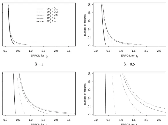
depend on por the prior mean. Figure 2 shows the relationship between the number
of failures and the ERPCIL criterion value, using the same combinations of cvη and
β entries used in Table 1.
We can see that, for given Weibull shape parameter and prior information, the relationships between the criterion value and number of failuresr are similar to those of the LSAPPF criterion, except for the scale difference. Because both (6) and (8)
reflect relative precision (not depending on the value of tp to be estimated), the
interpretation of these results from (8) are almost identical to those discussed in the previous example, using the LSAPPF criterion in (6).
As a direct comparison between the ERPCIL and LSAPPF criteria, Table 2 gives the needed numbers of failures based on these relationships for a certain specified criterion value, for selected combinations of prior information and the Weibull shape
0.0 0.5 1.0 1.5 2.0 2.5 ERPCIL for tp 0 1 02 0 3 04 0 5 0 number of failures β = 5 cvη = 0.1 cvη = 0.2 cvη = 0.5 cvη = 1 cvη = ∞ 0.0 0.5 1.0 1.5 2.0 2.5 ERPCIL for tp 0 1 02 0 3 04 0 5 0 number of failures β = 2 0.0 0.5 1.0 1.5 2.0 2.5 ERPCIL for tp 0 1 0 2 03 04 0 5 0 number of failures β = 1 0.0 0.5 1.0 1.5 2.0 2.5 ERPCIL for tp 0 1 0 2 03 04 0 5 0 number of failures β = 0.5
Figure 2: Needed number of failures as a function of ERPCIL fortp, when the Weibull shape parameter β is given and α= 0.05.
parameter. Note that, corresponding to R = 1.5, the relative credibility interval length from the large sample approximation is (tp×R−tp/R)/tp = 5/6. The test solutions from the two criteria only differ slightly, showing that the large sample approximation on which the precision factor R is based works quite well for this life test planning problem.
Table 2: Needed number of failures r based on the ERPCIL criterion in (8) and the
LSAPPF criterion in (6) for different prior cvη and Weibull shape parameterβ
prior cvη criterion value β ∞ 1.0 0.5 0.5 r= 88 r= 84 r= 71 5/6 for ERPCIL in (8) 1.0 r= 22 r= 21 r= 18 2.0 r= 6 r= 5 r = 4 0.5 r= 90 r= 86 r= 74 1.5 for LSAPPF in (6) 1.0 r= 22 r= 21 r= 18 2.0 r= 5 r= 5 r = 4
4.4
Discussion
The examples in this section explored the life test plans based on two different crite-ria: the LSAPPF criterion, based on the large-sample approximate Bayes credibility
interval precision factor R and the ERPCIL criterion, based on the relative Bayes
credibility interval length with respect to the mean. Both are relative precision met-rics, and neither depends on the particular value of p corresponding to the quantile of interest or the prior mean of the unknown Weibull scale parameter. The criterion based on the relative Bayes credibility interval length describes relative estimation precision in a more exact way.
We also computed a preposterior Bayes credibility interval length based on a large sample normal approximation, Et[2z1−α/2
VarP osterior(tp)], and a preposterior exact Bayes Length of (7), Et[Lα(tp|t)]. The latter is an average length criterion (ALC) like that proposed by Joseph, Wolfson and Berger (1995a,b). For design purposes, these criteria take the marginal expectation of the data to account for all possible outcomes of the data. These are absolute precision criteria, and they also lead to test plans that are close to each other. Because they are less frequently used in practice for planning to estimate positive quantities, the results are not presented in this paper.
4.5
Comparison with Non-Bayesian Test Plans
In the non-Bayesian approach of the life test planning problem, it is typical to use the inverse of the Fisher information matrix as the large sample approximate variance-covariance matrix of the maximum likelihood estimators of the unknown parameters. In the Weibull Type II censoring case with a given shape parameter, the information onη is I(η) = E −∂2logL(β, η;t) ∂η2 = rβ 2 η2
where the fact that tβ ∼ Exp(ηβ) and T T Tβ ∼ Gamma(r, ηβ) is used to obtain the expectation (cf. Epstein and Sobel 1953). Then, it follows that
R = exp z1−α/2 √ r−1 1 /β , (14)
which is the Bayesian analog to the Bayes LSAPPF criterion (6). This
non-Bayesian criterion is similar to LSAPPF in that it depends on r rather than n and
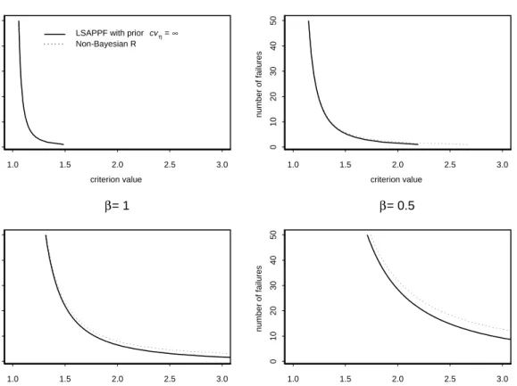
provides a relative precision metric. Figure 3 shows that the test solutions from this non-Bayesian R criterion are close to those from the LSAPPF criterion when prior cvη =∞, which is a non-Bayesian asymptotic case from Bayesian point of view. They
differ slightly from each other when r is small because LSAPPF uses the exact
1.0 1.5 2.0 2.5 3.0 criterion value 0 1 02 0 3 04 0 5 0 number of failures β= 5
LSAPPF with prior cvη = ∞
Non-Bayesian R 1.0 1.5 2.0 2.5 3.0 criterion value 0 1 02 0 3 04 0 5 0 number of failures β = 2 1.0 1.5 2.0 2.5 3.0 criterion value 0 1 0 2 03 04 0 5 0 number of failures β= 1 1.0 1.5 2.0 2.5 3.0 criterion value 0 1 0 2 03 04 0 5 0 number of failures β= 0.5
Figure 3: Comparison of the LSAPPF criterion for tp when prior cvη = ∞ and
non-Bayesian R criterion for tp, when the Weibull shape parameter β is given and
for the maximum likelihood estimator (the inverse of the Fisher information ma-trix). This establishes the correspondence between the Bayesian life test procedures obtained in Section 3 and non-Bayesian procedures.
5
Concluding Remarks and Areas for Future
Re-search
We have presented Bayes life test planning solutions for the Weibull lifetime distri-bution with a given shape parameter for Type II censored data. The closed forms of the planning criteria are easy to use in practice, and the solutions are meaningful for the practical problems where there is useful engineering information about the Weibull shape parameter. The results given here also provide an approximation to the case where a life test is terminated after a given amount of time (Type I censor-ing). In addition, the discussion of the criteria in this paper suggests that the large sample normal approximation works well for this Bayes life test planning problem and may also provide a simplified and effective approach for the more general case where the Weibull distribution parameters are all unknown. The large sample ap-proximation approach of the more general case, as well as some numerical validation such as simulation methods, should be explored in subsequent work.
A
Technical Details for Posterior Variance of
log(
t
p)
This section gives some technical details for the result in (5) in the body of the paper.
with shape parameter a and scale parameter 1, IG(a,1). Then, E(logX) = ∞ 0 (logx) 1 Γ(a) 1 xa+1 exp −1 x dx = − 1 Γ(a) ∂ ∂a ∞ 0 1 xa+1 exp −1 x dx = − 1 Γ(a) ∂ ∂aΓ(a) = −ψ(a),
where ψ(a) = Γ(a)/Γ(a) is the digamma function. Similarly,
E(logX)2 = 1
Γ(a) ∂2
∂2aΓ(a) = ψ
(a) + (ψ(a))2,
where ψ(a) =∂ψ(a)/∂a is the polygamma function. This leads to, Var(logX) = E(logX)2−(E(logX))2 = ψ(a). Because the posterior distribution of θ is IG(a+r, T T Tβ +b) in (2),
θ
T T Tβ +b ∼IG(a+r,1), from which (5) follows.
References
Adcock, C. J. (1997), The choice of sample size and the method of maximum
expected utility - comments on the paper by Lindley, The Statistician 46,
155-162.
Bernardo, J. M. (1997), Statistical inference as a decision problem: the choice of sample size, The Statistician46, 151-153.
Danziger, L. (1970), Planning censored life tests for estimation of the hazard rate
of a Weibull distribution with prescribed precision, Technometrics12, 408-412.
Epstein, B. and Sobel, M. (1953), Life testing,Journal of the American Statistical Association 48, 486-502.
Grubbs, F. E. (1973), Determination of number of failures to control risks of
erroneous judgements in exponential life testing, Technometrics15, 191-193.
Gupta, S. S. (1962), Life test sampling plans for normal and lognormal
distribu-tions, Technometrics 4,151-175.
Joseph, L., Wolfson, D. B. and du Berger, R. (1995a), Sample size calculations for binomial proportions via highest posterior density intervals, The Statistician
44, 143-154.
Joseph, L., Wolfson, D. B. and du Berger, R. (1995b), Some comments on Bayesian sample size determination, The Statistician 44, 167-171.
Joseph, L. and Wolfson, D. B. (1997), Interval-based versus decision-theoretic criteria for the choice of sample size, The Statistician46, 145-149.
Lindley, D. V. (1997), The choice of sample size, The Statistician 46,129-138. Meeker, W. Q. and Escobar L. A. (1998),Statistical Methods for Reliability Data, New York: John Wiley & Sons, Inc.
Meeker, W. Q., Escobar L. A., and Hill, D. A. (1992), Sample sizes for
estimat-ing the Weibull hazard function from censored samples, IEEE Transactions on
Reliability R-41,133-138.
Meeker, W. Q. and Nelson, W. (1976), Weibull percentile estimates and confidence
limits from singly censored data by maximum likelihood, IEEE Transactions on
Reliability R-25,20-24.
Meeker, W. Q. and Nelson, W. (1977), Weibull variances and confidence limits by
maximum likelihood for singly censored data, Technometrics19, 473-476.
Narula, S. C. and Li, F. S. (1975), Sample size calculations in exponential life
Nordman, D. and Meeker, W. (2002), Weibull prediction intervals for a future
number of failures. Technometrics 44,15-23.
Pham-Gia T. (1997), On Bayesian analysis, Bayesian decision theory and the
sample size problem, The Statistician 46,139-144.
Thyregod, P. (1975), Bayesian single sampling plans for life-testing with trunca-tion of the number of failures, Scandinavian Journal of Statistics 2,61-70. Zaher, A. M., Ismail, M. A., and Bahaa, M. S. (1996), Bayesian Type I censored designs for the Weibull lifetime model: information based criterion,The Egyptian Statistical Journal 40, 127-150.