Identification and estimation of nonlinear regression models using control functions

University of Warwick institutional repository: http://go.warwick.ac.uk/wrap

A Thesis Submitted for the Degree of PhD at the University of Warwick

http://go.warwick.ac.uk/wrap/50293

This thesis is made available online and is protected by original copyright. Please scroll down to view the document itself.

Identification and Estimation of

Nonlinear Regression Models

using Control Functions

Daniel Gutknecht

A thesis submitted in fulfillment of the requirements

for the degree of Doctor of Philosophy

University of Warwick

Department of Economics

Acknowledgements

I would like to thank my supervisors Valentina Corradi and Wiji Arulampalam for

their continuous encouragement and support throughout the PhD studies. Both

provided invaluable comments towards the completion of this thesis and taught me

crucial skills, without which I wouldn’t have arrived to this point. I am also very

thankful to both of them for having been patient with me and the way I delivered

work to them (more than once). Finally, I am particularly indebted to Valentina

Corradi for her fantastic support and advice during the job market phase.

I would also like to express my gratitude to Mark Stewart for his very useful

sugges-tions and his reference letter as well as to Jennifer Smith for her advice regarding the

collection of unemployment data from the British Household Panel Survey. Many

thanks also to S. Khan, Y. Shin, and E. Tamer for providing me with their GAUSS

routines from the paper Heteroscedastic Transformation Models with Covariate

De-pendent Censoring (JBES 2011, 29(1), p.40-48), which formed the basis of my own

GAUSS routines in Chapter two.

Finally, I am grateful to the Department of Economics for providing a stimulating

research environment and for the very generous funding support (my special thanks,

at this point, go to Abhinay Muthoo). Financial support from the ESRC and the

Royal Economic Society is also gratefully acknowledged.

The work of chapter two has been presented at Oxford, the University of Mannheim,

the University of Sydney, the University of Vienna, the LACEA-LAMES meeting in

Santiago (2011), the EEA-ESEM meeting in Oslo (2011), the University of Warwick,

and the Econometric Study Group Meeting in Bristol (2009). Comments received

from seminar participants (in particular from Steve Bond and Gerard van den Berg)

Declaration

This thesis is submitted to the University of Warwick in accordance with the

require-ments of the degree of Doctor of Philosophy. I declare that any material contained

in this thesis has not been submitted for a degree to any other university. Paper

versions of Chapter two and three have recently appeared in the working paper

se-ries of the Economics department at the University of Warwick (sese-ries no. 961 and

991).

Daniel Gutknecht

Contents

1 Introduction 1

2 Nonclassical Measurement Error in the Dependent Variable of a

Nonlinear Model 4

2.1 Introduction . . . 4

2.2 Setup . . . 8

2.2.1 Identification . . . 8

2.2.2 Estimation . . . 13

2.2.3 Asymptotic Properties . . . 17

2.2.4 Bootstrapping Confidence Intervals . . . 20

2.3 Monte Carlo Simulations . . . 22

2.4 Empirical Illustration . . . 25

2.5 Conclusion . . . 28

A2 Appendix . . . 31

A2.1 Assumptions . . . 31

A2.2 Proofs . . . 34

A2.3 Tables . . . 59

3 Do Reservation Wages Decline Monotonically? A Novel Statistical Test 62 3.1 Introduction . . . 62

3.2 Setup . . . 67

3.3 Large Sample Theory . . . 73

3.5 Monte Carlo Simulation . . . 82

3.6 An Application to Reservation Wages . . . 83

3.7 Conclusion . . . 90

A3 Appendix . . . 93

A3.1 Proofs . . . 93

A3.2 Tables & Figures . . . 99

List of Tables

2.1 Monte Carlo Simulation . . . 59

2.2 Monte Carlo Simulation - Censoring . . . 60

2.3 Empirical Illustration - Earnings Study . . . 61

3.1 Monte Carlo Simulation . . . 99

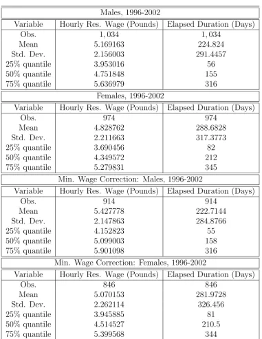
3.2 Descriptive Statistics . . . 100

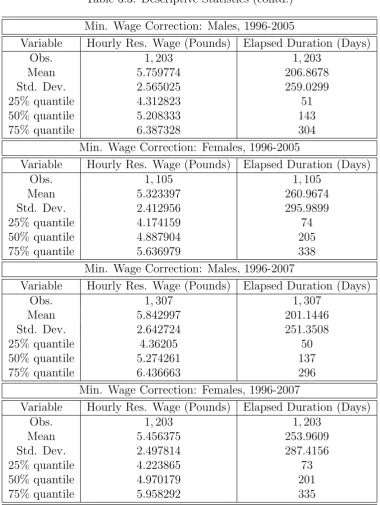
3.3 Descriptive Statistics (contd.) . . . 101

List of Figures

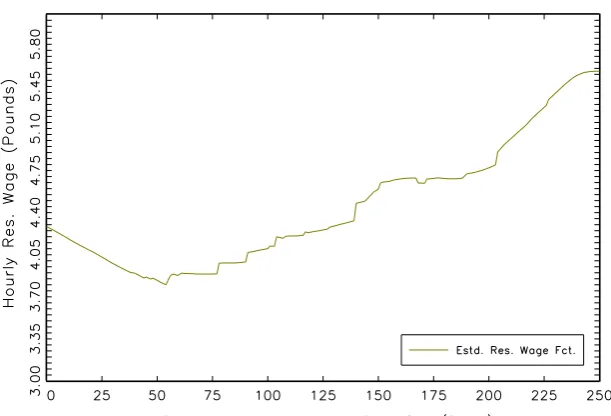
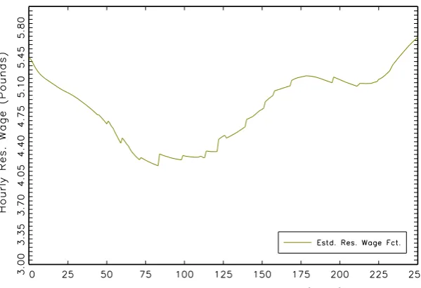
3.1 Men - Estimated Reservation Wage Function . . . 103

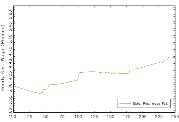
3.2 Men - Estimated Reservation Wage Function (contd.) . . . 104

3.3 Women - Estimated Reservation Wage Function . . . 105

1 Introduction

According to Blundell and Powell (2003), the development of strategies to identify

and estimate certain parameters or even entire functions of regression models under

endogeneity has arguably been one of the main contributions of

microeconomet-rics to the statistical literature. The term endogeneity, in this context, refers to a

correlation between observable regressor(s) and model unobservable(s), which can

arise for multiple reasons such as, among others, omitted variables, measurement

error, unobserved heterogeneity, or simultaneous causality. Whereas linear

identi-fication and estimation techniques to address endogeneity date back as far as 1928

(Stock and Trebbi, 2003), advances in the field of nonlinear models are much more

recent: nonlinear parametric models under endogeneity only came under

investiga-tion during the 1970s and 1980s (e.g. Ameniya, 1974; Hansen, 1982), and it was

not until the mid 1990s that models of (partially) unknown functional form were

considered.1

Literature focusing on endogeneity in the latter typically uses two different

iden-tification ideas that, despite the common assumption of an available instrumental

variable (vector), can be distinguished by the way identification is achieved:

non-parametric instrumental variable methods rely on the existence of a suitable moment

condition, which is based on the instrument(s) and in turn gives rise to an estimator

(e.g. Lewbel, 1998; Ai and Chen, 2003; Darolles, Fan, Florens, and Renault, 2011).

Control function methods on the other hand require the existence of a so called

control function, that is a function of the model observables and the instrument

(vector) satisfying a conditional (mean) independence assumption. Replacing the

control function by an estimated correspondent and incorporating this estimate into

1_{The general appeal of nonlinear models with (partially) unknown functional form for economics}

a suitable statistic to control for the endogeneity yields a consistent estimator of the

function or parameter of interest. Examples of this literature include e.g. Newey,

Powell, and Vella (1999), Blundell and Powell (2003), Imbens and Newey (2009) for

an extension to quantiles, and Blundell and Powell (2004) for an extension to binary

response models. Since both approaches are complements rather than substitutes

as the identification conditions do generally not imply each other, this thesis focuses

on the use of control functions as means to identify different semi- and

nonpara-metric regression models. In particular, the thesis contributes to the identification

literature of nonlinear models under endogeneity by examining two cases where the

correlation between regressor(s) and the model unobservable arises due to

measure-ment error (chapter two) and simultaneous causality between reservation wage and

elapsed unemployment duration (chapter three).

Specifically, chapter two studies nonclassical measurement error in the continuous

dependent variable of a semiparametric, non-separable transformation model. The

latter is a popular choice in practice nesting various nonlinear duration and censored

regression models. The main complication arises because the (additive)

measure-ment error is allowed to be correlated with a (continuous) component of the

regres-sors as well as with the true, unobserved dependent variable itself. This problem

has not yet been studied in the literature, but it is argued that it is relevant for

various empirical setups with mismeasured, continuous survey data like earnings

or durations. A framework to identify and consistently estimate (up to scale) the

parameter vector of the transformation model is developed. The estimator links a

two-step control function approach of Imbens and Newey (2009) with a rank

esti-mator similar to Khan (2001) and is shown to have desirable asymptotic properties.

Moreover, it is proven that ‘m out of n’ bootstrap can be used to obtain a consistent

approximation of the asymptotic variance. The estimator’s finite sample

perfor-mance is studied in a Monte Carlo Simulation. To illustrate the empirical usefulness

of the procedure, an earnings equation model is estimated using annual data from

the Health and Retirement Study (HRS) and its results are compared to the ones of

other estimators. Some evidence for a bias in the coefficients of years of education

error bias in empirical work.

Chapter three develops a test for monotonicity of a (possibly nonlinear) regression

function under endogeneity. The novel testing framework is applied to study

mono-tonicity of the reservation wage as a function of elapsed unemployment duration.

Hence, the objective of the chapter is twofold: from a theoretical perspective, it

proposes a test that formally assesses monotonicity of the regression function in the

case of a continuous, endogenous regressor. This is accomplished by combining

dif-ferent nonparametric conditional mean estimators using either control functions or

unobservable exogenous variation to address endogeneity with a test statistic based

on a functional of a second order U-process. The modified statistic is shown to have

a non-standard asymptotic distribution (similar to related tests) from which

asymp-totic critical values can directly be derived rather than approximated by bootstrap

resampling methods. The test is shown to be consistent against general alternatives.

From an empirical perspective, the chapter provides a detailed investigation of the

effect of elapsed unemployment duration on reservation wages in a nonparametric

setup. This effect is difficult to measure due to the simultaneity of both variables.

Despite some evidence in the literature for a declining reservation wage function over

the course of unemployment, no information about the actual form of this decline has

yet been provided. Using a standard job search model, it is shown that monotonicity

of the reservation wage function, a restriction imposed by several empirical studies,

only holds under certain (rather restrictive) conditions on the variables in the model.

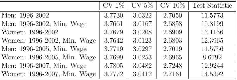
The test from above is applied to formally evaluate this shape restriction and it is

found that reservation wage functions (conditional on different characteristics) do

not decline monotonically.

Finally, all proofs and empirical results are postponed to the corresponding

Ap-pendix of each chapter. Numerical computations are carried out in GAUSS (routines

2 Nonclassical Measurement Error

in the Dependent Variable of a

Nonlinear Model

2.1

Introduction

The paper considers identification and estimation of the parameter vector of the

monotone transformation model (Han, 1987) when the continuous dependent

vari-able is subject to nonclassical measurement error, where ‘nonclassical’ refers to a

potential correlation of the measurement error with the true, unobserved

depen-dent variable itself and a (continuous) component of the regressor vector. This

setup is of interest from an empirical perspective as survey data is commonly

sub-ject to measurement error (Bound, Brown, and Mathiowetz, 2001). In particular

for earnings and duration data, evidence suggests that nonclassical measurement

error is the rule rather than the exception: Bricker and Engelhardt (2007) for

in-stance study measurement error in matched (annual) earnings data of older workers

in the Health and Retirement Study (HRS). Their findings suggest a strong

neg-ative (‘mean-reverting’) relationship between the extent of measurement error,

de-fined as the difference between self-reported survey and administrative records, and

‘true’ administrative earnings. According to their results for men of the 1991 wave,

measurement error falls by approximately $100 for each additional $1,000 in ‘true’

(administrative) annual labour income. In addition, measurement error is found

to cause a substantial upwards bias in the effect of education on annual earnings.

Cristia and Schwabish (2007) confirm both results using the Survey of Income and

Program Participation (SIPP) Panel matched to administrative records.1 _{In the}

1_{In addition, the study also provides evidence for a correlation of measurement error with other}

duration context, J¨ackle (2008) reveals a similar pattern for benefit recipient history

data from the ‘Improving Survey Measurement of Income and Employment’ project,

which employed (among other interviewing techniques) standard questioning

meth-ods from the British Household Panel Survey (BHPS) to infer about benefit receipts.

Using a non-representative sample and a proportional hazard model, she finds that

low educational attainment has a significant negative impact on the exit hazard of

benefit income related spells with survey data, but not with administrative records.

Moreover, under-reporting of the benefit duration (i.e. reporting a spell length that

falls below the actual length) generally increases when a spell spans more than one

survey wave.2 _{Since durations and earnings typically serve as ‘left-hand side’}

vari-ables in standard censored regression (e.g. Tobit) or duration models, which can be

nested within the monotone transformation model, both examples can be

accomo-dated by the framework developed in this paper.3 The paper addresses identification

and estimation of the “parametric” parameter vector of this transformation function

(up to scale). Future work will address the recovery of the unknown transformation

function, too.

The main contribution of this paper is to provide the researcher with a tool to

deal with nonclassical (as defined above) measurement error in continuous survey

data such as earnings or durations if the model of interest is the parameter

vec-tor of the monotone transformation model (or any other model nested therein).4

To the best of the author’s knowledge, such a tool does not yet exist. The main

theoretical complications in the identification and estimation process of the

param-eter vector arise because of (i) multiple unobservables (the measurement and the

equation error) in the model setup, (ii) the “lack” of assumptions on the

(condi-tional) measurement error distribution, and (iii) the potential dependence of the

measurement error and continuous component(s) of the regressors. In order to

ad-2_{More precisely, she finds that the share of self-reported durations longer than a year that end}

at the ‘seam’ of two survey waves exceed the share of corresponding spells from administrative records by 25−35% for certain benefit types.

3_{Notice that in order to apply the framework of this paper to the setup of Bricker and Engelhardt}

(2007), education needs to be modelled as a continuous variable (‘years of schooling’).

4_{The Proportional Hazard model can for instance be obtained by restricting the error term}

dress these points, a three-step identification and estimation procedure is proposed:

first, a two-step control function approach (see Blundell and Powell, 2003; Imbens

and Newey, 2009) is employed to solve the ‘endogeneity problem’ arising from the

dependence of the measurement error and a continuous component of the regressor

vector by estimating the conditional mean of the (mismeasured) dependent variable

conditional on all covariates and the estimated control function. Subsequently

inte-grating over the marginal support of the control function eliminates its impact as a

conditioning argument and reduces the measurement error to a numerical constant.

In a third step, a rank-type argument is then used comparing pairs of observations

to eliminate this numerical constant. Since a control function method is employed

in the first place, the procedure requires the existence of a suitable instrument

vec-tor. Also, notice that in particular the “lack” of assumptions on the (conditional)

distribution of the measurement error and the presence of multiple unobservables

prohibit the use of other control function estimators such as Rothe (2009). Instead,

all three steps outlined above are crucial for identification and consistent estimation

of the parameter vector.

Finally, it is argued that for the examples given before, instrumental variables

typ-ically suggested by the empirical literature for Mincer-type earnings equations such

as parental education, minimum school-leaving age, or (same sex) sibling’s

educa-tional qualification should also be applicable in this context as they are likely to be

correlated with the observed schooling level of the individual, but unlikely to affect

the individual’s actual response to the survey question.5 _{Moreover, as pointed out}

by Hu and Schennach (2008) and discussed in section 2.2.1, the choice of

instru-mental variables in the context of measurement error could even comprise repeated

measurements if certain conditions are met.

From a technical point of view, the main innovation of the paper is to combine

a nonparametric mean estimator with a rank estimation procedure and to derive

its asymptotic properties.6 _{Since duration models are arguably one of the most}

5_{Notice that this argument is valid even when measurement error is actually not related to}

cognitive ability but to other unobserved determinants.

6_{Concurrently to this work, Jochmans (2010) developed a two-step rank estimator for the}

relevant application field of the transformation model in practice, the estimator is

extended to allow for random right censoring. The additional estimation step

re-quired to accomodate censoring and to obtain the mean function further complicate

the asymptotic variance expression, which depends on first and second order

deriva-tives of certain conditional expectations. Thus, in order to construct confidence

intervals for the parameter estimates, the use of ‘m out of n’ bootstrap is suggested

to obtain corresponding standard errors and show their first order validity. Finally,

to illustrate the methodology empirically, annual earnings data from the HRS is

examined, which has been found to be subject to nonclassical measurement error

(Bricker and Engelhardt, 2007). A reduced version of an earnings equation is

esti-mated and it is found that the estimator differs substantially from other estimators

obtained for comparison purposes. Together with evidence for a mean-reverting

non-classical measurement error in annual earnings in the HRS (see Bricker and

Engelhardt, 2007), this underlines the need to adjust for measurement error bias

when examining the determinants of annual labour income of older workers in the

HRS as estimates appear to be strongly affected.

This paper complements the existing literature on nonlcassical measurement error,

which has been rather limited regarding measurement error in the response

vari-able of nonlinear models. In the duration context for instance, researchers have

limited attention to either fully parametric duration models or classical forms of

measurement error (e.g. Skinner and Humphreys, 1999; Augustin, 1999; Abrevaya

and Hausman, 2004; Dumangane, 2007), both of which are problematic once the

restrictive setup fails to hold. A notable exception is the paper by Abrevaya and

Hausman (1999), who consider nonadditive, classical measurement error in the

de-pendent variable. However, relative to the approach proposed here, their setup

can-not incorporate a correlation of the measurement error with the true, unobserved

dependent variable itself, which often appears to be the more relevant problem in

practice. Abstracting from the duration context, Chen, Hong, and Tamer (2005)

have considered various semiparametric models under nonclassical measurement

er-ror (in the dependent as well as the independent variable(s)) using auxiliary

istrative data to infer about the conditional distribution of the true variables given

the mismeasured variables. Matzkin (2007) examines a completely nonparametric

framework, but her identification result hinges on the independence of the response

error and other model (un-)observables. Hoderlein and Winter (2010) on the other

hand use a structural approach to identify marginal effects of linear and nonlinear

models under measurement error in either the dependent or the independent

vari-able(s). While their methodology allows them to make detailed statements about

the determinants and implications of such a measurement error, the validity of these

claims clearly relies on the underlying model assumptions.

The paper is organised as follows: Section 2.2.1 outlines the identification

strat-egy. Section 2.2.2 deals with the corresponding multi-step estimation procedure,

its asymptotic distribution is derived in Section 2.2.3 and the validity of the

boot-strapped confidence intervals is established in Section 2.2.4. Finally, Section 2.3

explores the finite sample properties in a small scale simulation study and Section

2.4 concludes with an empirical illustration on annual earnings data from the HRS

Survey. All tables and proofs are postponed to the appendix.

2.2

Setup

2.2.1

Identification

The monotone transformation model (Han, 1987), which nests several duration and

censored regression models, is given by:

Y_j∗ =m(X_j0β0+j) (2.1)

whereY_j∗ is an unobserved, continuous scalar dependent variable,X_j0 ={X_j(c), X_j(d)}0

is a (dx ×1)-dimensional covariate vector with X

(c)

j

X_j(d) containing continuous (discrete) elements, and j is a scalar unobservable (independent of Xj). m(·) is

name.7 Without loss of generality, this function is assumed to be strictly increasing

in the following.

Into this setup, an additively separable, nonclassical measurement error ηj is

incor-porated, which is a scalar random variable:

Yj =Yj∗+ηj (2.2)

‘Nonclassical’ here refers to a potential correlation of the measurement error with the

true, underlying dependent variable and (continuous) component(s) of Xj. That is,

letting “⊥” denote statistical independence of two random variables and “6⊥” their dependence, the following assumptions are made:

• j 6⊥ηj and

• X1j 6⊥ηj, whereX1j ∈X

(c)

j .

X1j could possibly also represent a vector of continuous random variables for each

of which a reduced form equation such as the one in A1 below holds (e.g. Blundell

and Powell, 2004).8 _{However, in order to maintain a tractable setup, X}

1j will be

assumed to be a scalar random variable in the following. By contrast, continuity of

the endogenous component is crucial to the control function approach and cannot

be relaxed (see below).

Regarding the additivity assumption of the measurement error, notice that if Y_j∗ is a duration variable taking on positive values only, the expression in (2.2) can be

viewed as the log-transformation ofYej =Ye_j∗·η_ej, where both Ye_j∗ andη_ej have support

[0,∞) and Ye_j∗, e

ηj >0 except for a set of measure zero. The assumption of additive

separability is hence not as restrictive as it might appear at first sight and has in

fact been adopted by several authors in the literature (e.g Chesher, Dumangane,

and Smith, 2002).

7_{Notice that the lack of restrictions onm(·) (apart from monotonicity) only allows for}

identifi-cation up to a loidentifi-cation and size normalization (Sherman, 1993).

8_{Notice that the identification and estimation procedure of this paper is applicable even if, apart}

from the correlation with the measurement errorηj,X1j 6⊥j. That is, as long as the instruments

satisfy the independence requirement outlined in assumption A1 below,β0 can be recovered even

Combining (2.1) and (2.2) yields the observed equation:

Yj =m(Xj0β0+j) +ηj (2.3)

The object is to identifyβ0from (2.3). To achieve this, the existence of an instrument vector Z_j0 = (X₋0 _1j, Z₁0_j) is assumed, where X₋0 _1j refers to all exogenous elements except for X1j:

A1 there exists a (dz×1)-dimensional vectorZj0 = (X

0 −1j, Z

0

1j) (with dimension(Z1j)

≥1) such that

X1j =g(Zj) +Vj (2.4)

with g(·) a real-valued function that is differentiable in its continuous compo-nents (with non-zero derivative), _E[Vj] = 0, and

Zj ⊥j, ηj, Vj

.

Condition A1 is the “exclusion restriction” typically imposed in the control function

literature. It specifies that the correlation between X1j and ηj only runs through

a function Vj, the so called control function. As outlined before, continuity of

X1j is crucial in this context since, in the discrete case, the distribution of the

control function Vj and its relation with ηj will in general depend on Zj violating

independence between Zj and the model unobservables. Full independence of the

instrument vector Zj on the other hand is required since the model in (2.3) is

not additively separable in observables and unobservables. Notice also that the

setup in (2.4) allows for parametric or semiparametric restrictions: for instance,

the researcher might specify a single-index model of the form X1j = g(Zj0γ0) +Vj

with γ0 an unknown vector of parameters and g(·) either an unknown or known differentiable function.

Concerning the empirical examples given in the introduction, instruments suggested

Butcher and Case, 1994; Card, 2001; Ichino and Winter-Ebmer, 1999) are

applica-ble in the measurement error setup, too. However, in line with Hu and Schennach

(2008), it is stressed that also a repeated measurement of Y_j∗ could be understood as an instrument if it satisfied the independence assumption in A1. That is, if

the second observation (together with the possible error contained in that

alter-native measurement) was independent of the measurement error ηj in the original

Yj conditional on the regressors Xj, the repeated measurement could become a

valid instrumental variable (see Chalak and White (2011) for a detailed discussion

of identification under various instrument concepts). Finally, since the setup is

en-tirely nonparametric, it is well known that identification condition A1 does not imply

nor is it implied by the moment conditions imposed in the nonlinear instrumental

variable (NIV) literature.

The second condition required for identification is a “large support condition”, which

ensures sufficient variation in Vj given X1j.9

A2 W =X × V is a compact, non-empty set, where X is a subset in the interior of the marginal support of X, while V denotes the marginal support of V. Assume that the joint density on W is everywhere continuous and bounded away from zero.

Assumption A2 states that the marginal support ofVj is identical to its conditional

support for a compact subset X of the marginal support of X. As discussed in Im-bens and Newey (2009), this might be restrictive in applications where data is scarce

or instrumental variables do not vary sufficiently as the above assumption basically

requires sufficient strength of the latter. In practice, a verification of A2 can only be

carried out approximately on a case by case basis. For instance, various Kolmogorov

Smirnov tests on the conditional distributions of the estimated control function for

subsets of the data used in the illustration example of section 2.4 indicate that the

condition seems to be satisfied for at least a subset of the data. Still, condition

A2 remains a drawback in the setup of this paper and future work will be directed

9_{Notice that a further support condition similar to Cavanagh and Sherman (1998) will ensure}

towards identifying sharp bounds similar to Imbens and Newey (2009).

The third assumption sufficient for identification of β0 is a standard i.i.d. assump-tion:

A3 {Xj, Zj, j, ηj}nj=1 is an i.i.d. sample, where Yj and the endogenous component

X1j are generated according to (2.3) and (2.4), respectively.

In the following, let µ(x) :=R _E[Yj|Xj =x, Vj =v]fV(v)dv with fV(·) the marginal

density of Vj and recall that m(·) is strictly increasing in its argument. Given this

setup, we obtain the following lemma, which ensures that the limit of the objective

function, introduced in the next section, is uniquely maximized:

Lemma 1. Under assumptions A1, A2, and A3 and given (2.3) and (2.4) withm(·)

strictly increasing in its argument, we have for every x,x_e∈ X:

µ(x)> µ(_ex) if x0β0 >xe

0

β0

The proof of this lemma can be found in the appendix and proceeds in three steps:

firstly, the mean of Yj conditional on Xj and Vj is computed. Using conditional

independence between ηj and Xj given Vj, the ‘remainder term’ becomes E[ηj|Vj].

However, since no assumption about the distribution of_E[ηj|Vj] such asE[ηj|Vj] = 0

are made, an iterated expectations argument to obtain_E[ηj] is subsequently applied

by integrating over the support of Vj. That is, it is shown that for every x ∈ X:

µ(x) =_E[m(x0β0+j)] +E[ηj] (2.5)

where the expectation is taken w.r.t. j and ηj, respectively. Notice that E[ηj] is

‘reduced’ to a numerical constant (which could be non-zero) and that µ(x), by the properties of m(·), is strictly increasing in x0β0 for allx ∈ X. The latter motivates the use of a rank-type argument (see Cavanagh and Sherman, 1998), which together

for every x∈ X and i, j ∈1, . . . , n:

E[m(x0β0+j)] +E[ηj] =E[m(x0β0+i)] +E[ηi]

Thus, givenxan inequality will only arise for differingβ-values. Moreover, it is clear from the above argument that the lack of structure on the transformation function

only allows for point identification of β0 in relative, not in absolute terms (that is, a normalization of β will be required). However, notice that if the researcher is willing to make parametric assumptions about the functional form of m(·), the above identification argument can be strengthened and point identification can be

achieved even in absolute terms. Also, it becomes apparent that other estimators

using control functions such as Rothe (2009) are not applicable here: the lack of

information about _E[ηj|Vj] does not make a “normalization” of this conditional

expectation to zero innocuous, but further steps to identify the parameter vector of

interest are required.

Finally, notice that in a standard linear model with m(·) equal to the identity func-tion, the identification procedure becomes applicable to “nonclassical” measurement

error in the independent variable, too. For instance, let:

Yj =X1j +X2∗jθ0+j

with X2j =X2∗j +ηj and ηj 6⊥ X2∗j as well as ηj 6⊥j. In this case, given a suitable

instrument vector Zj satisfying A1 and A2, it holds that:

R

E

h

Yj

X1j = x1, X2j =

x2, Vj =v]fV(v)dv=x1+x2θ0+E h

j

i

+_Ehηj

i

θ0 so that an identical rank argument to above becomes applicable and θ0 is identified up to scale.

2.2.2

Estimation

The three-step estimation procedure is immediate from the previous identification

result:

(i) In a first step, Vbj is recovered from a nonparametric first-stage regression of

(ii) Then, µ(x, v) := _E[Yj|Xj = x, Vj = v] can be estimated nonparametrically

using Yj, Xj,Vb_j and the average: b

µ(x) = _n1

n

P

i=1b

µ(x,Vb_i) for every x∈ X can be computed.

(iii) Finally, a modified version similar to the two-step rank estimator of Khan

(2001) can be used to recover β0 (up to scale).

The last step is similar to a modified rank estimator of Khan’s (2001), who uses an

estimated conditional quantile function as transformation of the dependent variable.

We replace this conditional quantile function and its estimator by the conditional

meanµ(x) and _bµ(x), respectively. The replacement (together with the introduction of a control function and censoring) affects the asymptotic variance of our estimator,

which will be different from the expression derived in Khan (2001), who does not

address endogeneity or random right censoring in his setup.

The estimated control functionsVbj stem from the regression equivalent of (2.4):

b

Vj =X1j−bg(Zj)

To estimateg(·), the Nadaraya-Watson estimator is proposed (for simplicity, assume that dz = 1) with

b

g(Zj) = n

P

k=1

X1kkh(Zj −Zk) n

P

k=1

kh(Zj−Zk)

where

kh(Zj −Zk) = k

Zj −Zk

h

and h is a deterministic sequence satisfying h −→ 0 as n −→ ∞, while k(·) is a kernel function that satisfies the restrictions in B3 in Appendix A2.1.10 _{An optimal}

bandwidth theory for the estimator is not developed in this paper, but instead

standard rules of thumb are employed for the determination of the bandwidth in

sections 2.3 and 2.4. Notice that g(·) could also be estimated by series estimators (splines, power series) or local linear smoothers, but the use of the Nadaraya Watson

10_{In practice, if some components of the instrument vectorZ}

j are discrete, nonparametric

estimator will facilitate several proofs in the appendix.This argument becomes even

more important as the limiting distribution obtained in section 2.2.3 does not depend

on the nonparametric first step estimators (a similar result was obtained by Newey

(1994) for smooth objective functions with a nonparametric plug-in estimate).

The conditional mean function µ(x) can be estimated using again the Nadaraya-Watson kernel estimator. Since the dx-dimensional covariate vector Xj contains dc

continuous elements and a univariate Vbj, the following d = (dc + 1) dimensional

product kernel is defined (for simplicity assume that: h=h1 =h2 =...=hd):

Kh,j(x, v) =k

x1−X1j

h

!

×. . .×k xdc−Xdcj

h

!

×k v−Vbj

h

!

and the following shorthand notation for the first dx elements is introduced:

Kh(x−Xj) = k

x1−X1j

h

!

×. . .×k xdc −Xdcj

h

!

To bound the denominator away from zero and to ensure that observations lie within

the compact set W, a nonrandom trimming function is introduced:

Ixi :=I[x∈ X, Vi ∈ V] and Ib_xi :=I[x∈ X,Vb_i ∈ V]

Notice that for simplicity no random trimming is employed, but different trimming

techniques might be used in practice.

Finally, in order for the estimator to become applicable in the duration context, the

possibility of random (right) censoring is accomodated into the estimation procedure

of the conditional mean by using the so called “synthetic data” approach of Koul,

Susarla, and van Ryzin (1981).11 As outlined in section 3.1, duration data is typcially

subject to (random) right censoring. Instead of observing the mismeasured duration

Yj for each individual, one typically observes:

Uj = min{Yj, Cj} and ∆j =I{Yj ≤Cj}

11_{The setup of this paper cannot straightforwardly be extended to fixed censoring. However, it}

where Cj is the censoring time and ∆j a censoring indicator. We assume {Cj,∆j}

to be independent of the other model covariates. This assumption, albeit debatable

in some settings, is standard in the literature and often justified in practice. In

addition, define:

UjG=

Uj∆j

1−G(Uj−)

and

U_j

b

G=

Uj∆j

1−Gb(U_j−)

where G(·−) is the left-continuous distribution function of Cj and Gb(·−) the cor-responding Kaplan-Meier estimator (Kaplan and Meier, 1958) with Hb(·−) the left-continuous empirical distribution function of Uj:

b

G(c) = 1− Y

i:Ci≤c

1−

Pn

j=1I[(1−∆j) = 1, Cj ≤Ci] 1−Hb(U_i−)

!1−∆i

Replacing the partially unobserved Yj byUjG, Koul, Susarla, and van Ryzin (1981)

showed that under condition B1 in appendix A.1:

E[UjG|Xj =x, Vj =v] =E[Yj|Xj =x, Vj =v] (2.6)

Since UjG is unobserved, we can replace it by UjGb and estimate (2.6) as:

b

µ(x,Vbi) = n

P

j=1 b

IxiUjGbKh,j(x,Vbi)

n

P

j=1 b

IxiKh,j(x,Vbi)

(2.7)

while:

b

µ(x) = 1

n

n

X

i=1 b

µ(x,Vb_i) (2.8)

is the average of µ_b(x,Vb_i) over Vb_i. The last stage recovers the parameter vector β₀. As rank estimators only allow an identification of β0 up to scale, a normalization of an arbitrary component of the parameter vector is required. Following standard

procedures, the first component is normalized to one, i.e. β(θ)≡(1, θ).12 Thus, the

12_{Accordingly, the true parameter vector isβ(θ}

third stage rank estimator is given by:

β(bθ) = arg max

θ∈Θ 1

n(n−1) X

k6=l

I[Xk∈ X]×µb(Xk)×I[X

0

kβ(θ)≥X

0

lβ(θ)] (2.9)

where P

k6=l stands for the double sum

Pn

k=1 Pn

l>k assuming that observations are

in ascending order.13 _{The form of (2.9) is almost identical to the two-stage rank}

estimator of Khan (2001) using a conditional mean instead of a conditional quantile

function. Notice that for the above estimator to work we require thatµ_b(Xk)>0 for

every Xk inX. Thus, if Yj also takes on negative values, an upfront transformation

of the data needs to be carried out, e.g. Yj = Yj − min{Y1, . . . , Yn}, to ensure

positivity.

2.2.3

Asymptotic Properties

This subsection considers the asymptotic properties of the estimation procedure.

The probability limit of (2.9) evaluated at θ0 is:

Z

I[Xk ∈ X]×µ(Xk)×I[Xk0β(θ0)≥Xl0β(θ0)]dFX(Xk, Xl) (2.10)

where FX(·,·) in this case denotes the distribution function of Xk, Xl. Since the

conditions for consistency, √n-consistency, and asymptotic normality are standard and rather lengthy (see Cavanagh and Sherman (1998) or Khan (2001) for details),

the reader is referred to Appendix A.1 for details, where conditions B1 to B8 used

in the theorems below are outlined together with a short discussion of non-standard

assumptions. Notice that a higher order kernel function is employed in order to

allow for a fairly large dimension of the covariate vector Xj. That is, with an

increasing number of covariates used in the estimation of the conditional mean, a

kernel function with an increasing number of moments equal to zero is required in

order to control for the asymptotic bias.

13_{Summations appearing in the following that involve more than two indices will be defined}

Theorem 2. Under conditions A1-A3, B1-B5, B7, and B8, we have:

b

θ →p θ0

The proof of Theorem 2 parallels the proof of Theorem 3.1 in Khan (2001). The

main difference with respect to the latter is to show that replacing µ_b(Xk) by its

probability limitµ(Xk) results in an error of smaller order for everyXk ∈ X. Unlike

Khan (2001), however, also the estimated termsVb_j,U_j b

G, andIbj need to be controlled

for. One difficulty arises as theVbj also enter the indicator functionIbj, which in turn

prevents a Taylor expansion. An argument from Corradi, Distaso, and Swanson

(2011) is borrowed to show that this term can in fact be bounded by an expression

approaching zero at rate ln(n)12/(nhdz) 1

2 −→0. Together with the convergence rates of U_j

b

G and Vbj, the overall rate is:

b

µ(x)−µ(x) =Op

ln(n)

nhdz

!1₂!

=op(1)

for every x∈ X.

Given consistency of θbforθ0, one can replace the parameter space Θ by a shrinking set around θ0 to establish

√

n-consistency and asymptotic normality using results of Sherman (1993). To simplify notation in the next theorem, the following expression

is defined (see Khan, 2001; Sherman, 1993):

ψ1(x, θ) = Z

µ(x)×I[x∈ X]I[x0β(θ)> u0β(θ)]−I[x0β0 > u0β0]dFx(u)+

Z

µ(u)×I[u∈ X]I[u0β(θ)> x0β(θ)]−I[u0β0 > x0β0]dFx(u)

(2.11)

Moreover, denote:

ψ2(x, θ) = Z

I[x∈ X]I[x0β(θ)> u0β(θ)]dFx(u) (2.12)

Theorem 3. Under conditions A1-A3 and B1-B8, it holds that:

√

n(bθ−θ0)

d

where Σ =J−1ΩJ−1 with:

J = 1 2E

∇_θθ0ψ₁(X_k, θ₀)

The diagonal elements of the matrix Ω are given by the sum of the following

expres-sions:

(i)

Ω0 = Z

Im(UmG−µ(Xm))∇θψ2(Xm, θ0)

×Im(UmG−µ(Xm))∇θψ2(Xm, θ0) 0

dFUG,X,V(UmG, Xm, Vm)

(ii) Ω1 =E1Φ1E

0

1 with:

Φ1 = Z

V_i2dFV(Vi)

and

E1 =

F_V(1)a+F_V(1)b

Z

UjG∇θψ2(Xk, θ0)dFUG,X(UjG, Xk)

where a, bare real numbers andF_V(1)(·)denotes the first-order derivative of the distribution function FV(·) of V.

(iii) Ω2 =E2Φ2E

0

2 with

Φ2 = Φ1

and

E2 =− Z

IiUjG∇θψ2(Xk, θ0)dFUG,X,V(UjG, Xk, Vi)

(iv) Ω3 =E3Φ3E

0

3 and

Φ3 = Z φY

0

E

h

U1GI[s < U1] i

Ht1(s)

dG(s) (1−G(s−))

and

E3 = Z

where φY is defined in B1 and Ht1(s) =E

h

U1GI[s < U1] i

/{(1−FY(s−))(1−

G(s−))}.

The proof of Theorem (3) follows the proof of Theorem 3.2 in Khan (2001). The

conditions of Lemmata A.1 and A.2 therein are explicitly verified, which establish

√

n-consistency and asymptotic normality, respectively. The main differences to Khan (2001) consist in the use of a conditional mean rather than a conditional

quantile function and in the estimated first and second stage terms Vbj, Ibj, and U_jGb, which complicate the asymptotic analysis in this case further. Both, the estimation

of the conditional mean function as well as the estimated Vbj, Ibj, U_jGb yield the extra pieces Ω0, Ω1, Ω2, and Ω3 in the variance-covariance matrix Σ that differ

from the expression derived by Khan (2001). The first step in the proof of the

above theorem is to replace µ_b(Xk) in (2.9) by µ(Xk). The term involving µ(Xk)

can be expanded to yield the gradient J = 1_2E

∇_θθ0ψ₁(X_k, θ₀) plus terms that

are of order op(n−1) once

√

n-consistency of kθb−θ₀k has been established (notice that Lemmata B.1 and B.2 are verified concurrently and hence expressions shown

to be of order op(kbθ −θ₀k/

√

n) for instance automatically become op(n−1) once

kθb− θ₀k = O_p(1/

√

n) has been established via Lemma B.1). The second term containing the estimation error (µ_b(Xk)−µ(Xk)) on the other hand can be further

expanded to give the different variance pieces plus terms that are again of order

op(n−1) on a set around θ0 shrinking at rate

√ n.

2.2.4

Bootstrapping Confidence Intervals

The asymptotic variance depends on moments of the derivatives of the unknown

functionsψ1(·,·) andψ2(·,·), which can be estimated using either numerical deriva-tives (e.g. Sherman, 1993; Cavanagh and Sherman, 1998) or kernel-based methods

(Abrevaya, 1999). However, since these moments may be difficult to estimate in

practice, the use of the ‘m out of n’ bootstrapping procedure is proposed as an

alternative to construct standard errors for our parameter estimates. The ‘m out

of n’ bootstrapping procedure is a widely applicable methodology allowing to

bootstrap method is able to replicate the degeneracy of first order terms from the

linear U-statistic expansion (Arcones and Gine, 1992) that is used multiple times in

the derivation of the asymptotic distribution of our estimator. The nonparametric ‘n

out of n’ bootstrap method fails to replicate this degeneracy and hence an extension

of the setup in Subbotin (2008), who recently showed that nonparametric ‘n out of

n’ bootstrap methods consistenly estimate variances and quantiles of standard rank

estimators, is not pursued in this paper.

The procedure works as follows: X₁∗, . . . , X_m∗ and Z₁∗, . . . , Z_m∗ are sampled from the original sample of size n (with m < n) and Vb₁∗, . . . ,Vb_m∗ are obtained. In total, 1, . . . , B of these bootstrap samples of size m are constructed. For each of these samples, the bootstrap equivalent of our estimator is computed:

β(θ∗) = arg max

θ∈Θ

1

m(m−1) X

k6=l

I[X_k∗ ∈ X]×µ_b∗(X_k∗)×I[X_k∗0β(θ)≥X_l∗0β(θ)] (2.13)

where

b

µ∗(X_k∗) = 1

m

m

X

i=1 (

m

P

j=1 b

I_ki∗U∗

jGb

Kh∗_,j∗(X_k∗,Vb_i∗)

m

P

j=1 b

I_ki∗Kh∗_,j∗(X∗

k,Vb_i∗) )

and the bandwidth sequence h∗ is in lieu ofhfrom Section ??shrinking to zero at a rate depending on m (rather than n). Hence one obtains θ₁∗, . . . , θ_B∗. The aim is to construct a 1−αconfidence interval (CI) from the empirical bootstrap distribution. Thus, one needs to recover standard errors from the bootstrap covariance matrix,

which is given by:

Σ∗ = m

B

B

X

i=1

θ_i∗− 1 B

B

X

i=1

θ_i∗

θ∗_i − 1 B

B

X

i=1

θ∗_i

0

The next theorem establishes that Σ∗ is a consistent estimator for Σ:

Theorem 4. Let _P∗ denote the probability distribution induced by the bootstrap

sampling. Under assumptions A1-A3 and B1-B8 with h∗ and m in place of h and

n, respectively, and letting m, n,_mn −→ ∞, it holds for all >0:

P

ω:_P∗

Σ∗−Σ

>

In order to prove the above theorem, it is firstly verified that √m(θ∗ −θb) has the same limiting distribution as √n(bθ−θ0) in a similar manner to before. However, since first order validity does not justify the use of the variance of the bootstrap

distribution to consistently estimate the asymptotic variance (e.g. Goncalves and

White, 2004), it is also shown that uniform integrability holds as well. A sufficient

condition for the latter is the existence of a slightly higher moment condition, which

in turn ensures consistency of the bootstrap variance estimator.

2.3

Monte Carlo Simulations

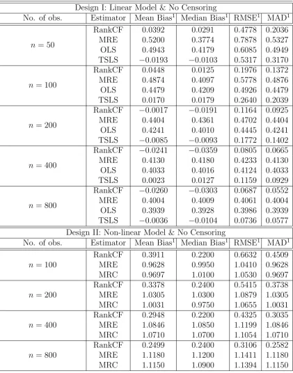
To shed some light on the small sample properties of the estimator in 2.9, various

Monte Carlo simulations are conducted. The results are displayed in Table 2.1 and

2.2 of Appendix A2.3. The analysis starts by looking at a linear model under

non-classical measurement error (as defined in Section 2.2.1) in the dependent variable.

This allows to compare the performance of the estimator proposed in this paper

relative to other estimators that are consistent (Two Stage Least Squares) or

incon-sistent (Monotone Rank Estimator, Ordinary Least Squares) in a linear setup.

More precisely, a linear model with two independent variables X1j and X2j is

exam-ined:

Y_j∗ =X1j+X2jθ0+j

with the coefficient of X1j normalized to one and θ0 set equal to .5. The additive measurement error ηj is given by:

Yj =Yj∗+ηj

The model unobservables j and ηj are generated through a multivariate normal

distribution:





j

M j



∼N 

 0

0 

; 



1 −.5

−.5 1 

 !

and the auxiliary equation ηj = κ·Vj +Mj with κ = .5. The negative

empirical studies (Bound, Brown, and Mathiowetz, 2001). X1j is simulated from a

uniform distributionU[1,2], while X2j is determined by the following reduced form

model:

X2j =α·Zj +Vj

with α = 1. The instrument Zj and the control function Vj are simulated from

two uniform distributionsU[0,1] andU[−1,1], respectively. Notice that the chosen range of Zj and Vj imply that Vj has full support given 0≤x2j ≤1.

The estimator (labelled RankCF) proposed in section 2.2.3, which is consistent forθ0, is compared to various other estimation procedures: the Two Stage Least Squares

estimator (TSLS), which is also consistent in the linear model setup, is used to

evaluate the relative performance of the RankCF in small samples. These results

are contrasted with results from the inconsistent Ordinary Least Squares estimator

(OLS) and the likewise inconsistent Monotone Rank Estimator (MRE) introduced

by Cavanagh and Sherman (1998).14 The latter has been chosen as it forms the basis

for the RankCF and, like the RankCF, also requires an optimization algorithm due

to the discontinuous character of the objective function. The chosen algorithm is the

Nelder-Mead Simplex method with the normalized TSLS results as starting values.

The sample size varies from 50, 100, 200, 400 to 800 observations. For every sample

size, 200 replications are conducted. The displayed deviation measures are Mean

Bias, Median Bias, Root Mean Square Error (RMSE), and Mean Absolute Deviation

(MAD). They are constructed as averages over the number of replications. A second

order Epanechnikov kernel is employed using the rule of thumbstd(·)·n−71.5 for the bandwidth selection, where std(·) is the standard deviation of the corresponding argument, while n remarks the sample size.

Starting with the simulation results in Table 2.1 (Design I: Linear Model & No

Censoring), one can observe that even at small sample sizes TSLS and RankCF

perform well across all bias measures (with a slight advantage for TSLS). Moreover,

in line with consistency, their Mean Bias, RMSE, and MAD shrink as the sample

size increases (albeit not gradually for the Mean Bias). This is not the case for the

MRE and OLS, where the mean bias is still of order .4 even at n= 800.

Next a non-linear design is examined. Using again Yj = Yj∗ +ηj, the non-linear

model is chosen to be:

Y_j∗ = ln(X1j +X2jθ0+j)

with X2j, and j being determined as before, while X1j ∼ U[2,3]. Notice that in

this nonlinear setup with nonclassical measurement error, all estimators except for

the RankCF estiamtor are inconsistent either due to the non-linearity or due to

the endogeneity of X2j. OLS and TSLS will be dropped from the set of estimators

and instead be replaced by the Maximum Rank Correlation Estimator, which was

introduced by Han (1987) as the first estimator in the literature using a rank-type

argument. The results are displayed in the lower part (Design II) of Table 2.1. Again,

one can observe that the theoretical predictions are largely confirmed. Despite

a relatively poor performance of all three estimators at n = 50, the bias of the MRE and the MRC remain substantial as n increases (albeit a certain decrease in the RMSE and MAD). This is not the case for the RankCF, where the mean

bias decreases as the sample size increases (even though the bias has not entirely

disappeared at n= 800).

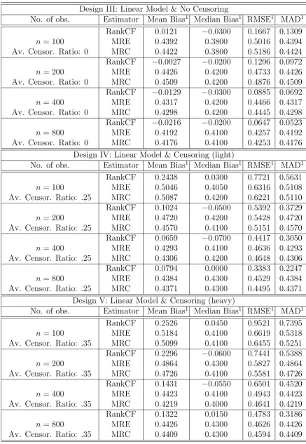
Finally, the censoring setup in Table 2.2 is examined comparing our estimation

procedure again to its rank competitors, the Monotone Rank Estimator (MRE)

and the Maximum Rank Correlation Estimator (MRC). Notice that, in addition

to the inconsistency because of the correlation between X2j and ηj, the MRE as

well as the MRC have not been formally extended to the case of random right

censoring. To evaluate the relative performance of our censoring adjustment, we

firstly carry out the simulations for the linear model of Design I without censoring

(but X2j ∼ U[2,3]). To maximize the objective functions, we revert again to the

above grid search method. The two censoring cases are also built upon the linear

setup of Design II and contain two different average censoring ratios, .25 and .35. The censoring variable Cj is sampled from a uniform distribution U[1,6] (Design

IV) and U[1,8] (Design V), respectively. Notice that the support of Cj ‘covers’

Turning to the simulation results, one can see that the effect of censoring drives up

the biases particularly at small sample sizes. Somewhat surprisingly, the negative

impact appears most pronounced for the method proposed in this paper, even though

the deterioration slowly vanishes as the sample size increases. Despite this more

negative effect of censoring, one can observe that, as expected from a theoretical

perspective, the difference in mean and median bias is substantial for all sample

sizes excelling the MRE and the MRC in particular for the case of ‘light’ censoring

(Design IV). As the censoring ratio increases, all bias measures become fairly large.

Once again, however, one observes a substantial improvement for the RankCF with

the size of the sample growing, while the bias measures do only moderately change

for the MRE and the MRC.

Overall, the results from this small simulation study indicate a good finite

sam-ple performance of the methodology for the chosen setups under different forms of

nonclassical measurement error and various degrees of censoring.

2.4

Empirical Illustration

In a recent study, Bricker and Engelhardt (2007) provided empirical evidence for

nonclassical measurement error in annual earnings data from the Health and

Retire-ment Study, which is a nationally representative longitudinal survey of the over 50

population in the US.15 _{The researchers found a mean-reverting pattern in the data}

and a significant positive correlation between higher education and measurement

error. The mean measurement error (defined as the difference between self-reported

HRS and matched administrative annual earnings) was found to be approximately

$1,500 with a standard deviation of $13,899, which is substantial given that the

mean of self-reported and administrative earnings stood at $33,584 and $32,071,

respectively. The authors also established that for every additional $1,000 in ‘true’

earnings, measurement error fell by $100. Finally, men with a college degree or

higher earned 49.2% more than high-school drop-outs based on reported earnings,

15_{See the University of Michigan’s webpage http://hrsonline.isr.umich.edu/index.php for a}

but only 42.1% more based on the matched administrative annual earnings. Unlike

in the paper of Bricker and Engelhardt (2007), the 1998 wave is chosen, which also

includes the ‘War Babies’ and the ‘Children of the Great Depression’ cohorts to

broaden the age range in the data and to comply with the assumption of a

contin-uous variable in the covariate vector. The sample is restricted to individuals with

positive labour income during that year (i.e. no self-employed) and individuals that

were the actual financial respondents of the household.16 Moreover, to further

en-sure a certain degree of homogeneity, only white individuals are selelcted for the

final dataset. The full support requirement in the assumption setup also meant

that persons below the age of 50 and above 70, and those with less than 10 years of

schooling were excluded.17 The final sample size comprised 2,753 observations.

For the earnings equation, (natural) logarithm of annual labour income is taken to

be the dependent variable and gender, age (as a proxy for experience), age squared,

and years of schooling are considered as model covariates.18 _{In a linear setup, using}

years of schooling as independent variable embeds the assumption of log earnings

being a linear function of education, i.e. each additional year of education having the

same proportional effect on expected annual earnings. Notice that this constraint

does not apply to here though as the model setup allows for a nonlinear, monotonic

transformation function. It does only apply to the interpretation of competing

estimators imposing a linear model. The possibility of measurement error in the

independent variables (which can certainly be put into question) is ruled out and

the coefficient of gender is normalized to one as it is a well known result that being

a male has a positive effect on earnings. As instruments for the respondent’s years

of schooling we choose years of schooling of the mother and the father, respectively.

These family background covariates are typically correlated with the schooling level

16_{Annual labour income comprises (i) regular wage or salary income, (ii) bonuses, tips,}

commis-sions, extra-pay from overtime, (iii) professional practice or trade earnings, and (iv) other income earned from a second job or while in the military reserves.

17_{Various Kolmogorov Smirnov tests were carried out to compare the conditional distributions}

of the estimated control function residuals for different subsets of the data. The results of these tests indicate that the assumption of a full support is roughly satisfied for this range of the data.

18_{Notice that the use of three regressors plus an (estimated) control function requires the}

of the individual, but unlikely to be related to the respondent’s actual misreporting

or his/ her ability.19

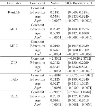
The estimation results are compared to the ones of the MRE and the MRC as well

as a Least Squares (OLS), a Least Absolute Deviations (LAD), and a Two-Stage

Least Squares (TSLS) estimator. The latter uses the mother’s and the father’s

ed-ucation as instrumental variables for the respondent’s years of schooling and serves

as an additional reference point for the education coefficient. Due to the

discon-tinuous character of the objective function, a Nelder-Mead Simplex method is used

to optimize the functions of the three rank estimators. As starting values for the

initial simplex the OLS estimates are chosen.20 _{To obtain a 90% confidence interval}

for the parameters, a ‘m out of n’ bootstrap with subsample size of 1.600 and 200

replications was conducted.

Examining the results in Table 2.3 in Appendix B, one observes that point estimates

of age and age squared of our estimator (RankCF) lie amid the range of competing

estimates from the MRE, MRC, OLS, LAD, and TSLS. This is in line with the

finding of Bricker and Engelhardt (2007), who did not find a correlation between

measurement error and age. Naturally, the use of first stage estimates in the final

estimator (RankCF and TSLS) does come at the price of larger confidence regions.

However, notice that the range of the confidence bands is fairly similar for the TSLS

and our estimation procedure, and all point estimates still appear to be significant

at a 10% level. Turing to the coefficient of interest, the education coefficient of

our estimator differs from its competitiors and falls substantially below their values

hinting at an upwards bias in the education coefficient of the other estimators. It can

of course not be established whether the size reduction in the estimated education

coefficient can be attributed to an elimination of the measurement error or the

standard ability bias (by standard arguments, one would expect the abilitiy bias

to be positive, which corresponds to the direction of the measurement error bias

as found by Bricker and Engelhardt (2007)). However, the relatively unchanged

19_{Despite criticism in the literature about the suitability of parental education as an instrumental}

variable for childrens’ education, it is deemed that these variables still serve the purpose of this small scale illustration.

20_{Notice that the results were rather insensitive to small variations in the initial simplex, e.g.}

TSLS estimate of the education coefficient suggests that measurement error might

be the reason for the drop in size. This conjecture is supported by the observation

that there are no substantial differences between the estimates of OLS and LAD on

one hand and MRE and MRC on the other, which suggests that a violation of the

linearity restriction is unlikely to be the driving force behind the difference between

the TSLS and the RankCF result.

Summarizing this small illustrative example that looks at a log earnings equation

with years of education, gender, age, and age squared as covariates using the 1998

wave of the HRS, it is found that point estimates for the education coefficient

pro-vided by the estimation procedure proposed in this paper differ quite substantially

from those of its competitors. Moreover, since the age coefficient of the estimatior

of section 2.2.3 is largely in line with the values obtained from the other estimators

(confirming Bricker and Engelhardt (2007), who did not find a substantial

correla-tion of measurement error with other characteristics such as age), the illustrative

results hint at the presence of measurement error bias in standard earnings equation

regressions based on the HRS. Together with the empirical evidence of Bricker and

Engelhardt (2007) for a mean-reverting non-classical measurement error in annual

earnings that is correlated with education (Bricker and Engelhardt, 2007) from the

1992 wave, this underlines the need to adjust for measurement error bias when

exam-ining the determinants of annual labour income of older workers in the HRS.

2.5

Conclusion

This paper proposes a multi-step procedure to identify and estimate the parameter

vector of the monotone transformation model when the continuous dependent

vari-able is subject to nonclassical measurement error. Empirical evidence examining

duration and earnings data collected via survey questionnaires often suggests that

such a measurement error represents the rule rather than the exception. Taking on

a reduced form perspective, a methodology to address measurement error when the

researcher does not dispose of any information about the underlying distribution of

she only has a suspicion about the correlation pattern of the latter. Combining a

modified control function approach, which requires the existence of a suitable

instru-mental variable vector, with a rank-type argument, it is shown that it is possible to

recover the aforementioned parameter vector consistently up to a location and size

normalization. We derive the estimator’s asymptotic properties and also

demon-strate the methodology’s good finite sample performance in a small Monte Carlo

Study. Finally, an empirical illustration investigating the effect of years of schooling

on annual (log) earnings data from the Health and Retirement Study concludes this

paper. Substantially different point estimates are found using our estimation

proce-dure (relative to other estimators) suggesting that to account for correct inference

is important in this context.

Extensions of the present paper and topics for future research include the

non-parametric recovery of the unknown transformation function m(·), which requires a point identification result for the parameter vector hence providing another

mo-tivation for the asymptotic result derived in this paper. Being able to identify and

nonparametrically estimate the transformation function is of particular interest in

survival analysis, where the function is typically labelled ‘integrated baseline hazard’

and of substantial importance for policy analysis purposes. Alternatively, in

con-texts where the large support assumption appears to be unjustifiable, the researcher

might instead be interested in abandoning the goal of point identification in favour

of sharp bounds on the parameter vector. Such an extension was considered by

Imbens and Newey (2009) in a similar setup and represents an important future

extension of the present work.

The case of measurement error in multiple spell duration models appears to be

an-other important area of future research, too: despite suitable stationarity

assump-tions on the measurement error (similar to the ones used in Abrevaya (2000) for

the idiosyncratic error terms), such an extension is more complex as ‘fixed effects’

estimators typically exploit ‘intra-unit’ variation rendering the integration over the

support of the control function more difficult. Finally, a last field of interest might

be the case of binary dependent variables: duration models in discrete time are

period takes on the value zero if the spell is on-going and one if the spell fails. Thus,

falsely reported or recorded responses turn the nonclassical measurement error into

a misclassification rather than a measurement problem, which is non-trivial due

to the nonlinear nature of the underlying model (Hausman, Abrevaya, and

A2

Appendix

A2.1

Assumptions

Letk·kdenote the Euclidean norm and∇ithe i-th order derivative of a function.

B1 Cj is i.i.d. and independent ofYj. Moreover,Cj satisfies:

(i) _P[Cj≤Yj|Yj=y, Xj=x, Vj=v] =P[Cj≤Yj|Yj=y].

(ii) G(·) is continuous.

(iii) φY ≤φC

with φY = inf{t : FY(t) = 1}, φC = inf{t : G(t) = 1}, and FY(t) = P[Yj ≤ t],

G(t) =P[Cj ≤t].

(iv) When φY < φC, lim sup t→φY

RφY

t (1−FY(s))dG(s))

1−ρ_/(1−F

Y(t)) < ∞, for some

2 5 < ρ <

1 2.

(v) WhenφY =φC, for some 0≤ς <1, (1−G(t))ς =O((1−FY(t−))) ast→φY.

(vi) LetFU(t) = P[Uj ≤ t] and H(Uj) =

RUj

−∞dG(s)/({1−FU(s)}{1−G(s)}). Assume

that:

Z

UjH

1

2+ε(U_j)[1−G(U_j−)]−1dF_U,X,V(U, X, V)<∞

B2 The elementsxin the support ofX can be partitioned into subvectors of discretex(d)_and

con-tinuousx(c)components. Let X(d) _{and X}(c) _{be the corresponding discrete and continuous}

parts ofX ⊂ W. Assume that the conditional density (givenx(d)∈ X(d)_{) onW is}

every-where continuous and strictly bounded away from zero. Moreover, assume that X is not contained in any proper linear subspace of_Rdx _{and that the subsetX}

(1) of one component

of thedx-dimensional setX =X(d)× X(c)contains the interval:

h

µ(x)−3 max

x0 (−1)θ

|x0₍₋₁₎θ| ; µ(x) + 3 max

x0 (−1)θ

|x0₍₋₁₎θ|i

for anyx∈ X, wherex(−1)denotes the remaining (dx−1) dimensional component and the

maximum is taken overX(−1)×Θ with max

x0 (−1)θ

|x0

(−1)θ|<∞.

B3 The multivariate kernel function K = k×. . .×k with K : _Rd _7−→

R is symmetric, has

compact support, and is differentiable (with bounded derivative). In addition,K(·) satisfies (i) R

K(u)du = 1, (ii) R

K(u)uγ_{du = 0 for γ = 1, . . . , r−1, (iii)} R

K(u)ur_{du 6= 0 and}

R

K(u)urdu <∞, (iv)R

|K(u)|du <∞, and (v)R

K2(u)du <∞.