energy path finding methods
Cite as: J. Chem. Phys. 150, 094109 (2019); https://doi.org/10.1063/1.5064465
Submitted: 04 October 2018 . Accepted: 13 February 2019 . Published Online: 05 March 2019
A preconditioning scheme for minimum energy
path finding methods
Cite as: J. Chem. Phys.150, 094109 (2019);doi: 10.1063/1.5064465 Submitted: 4 October 2018•Accepted: 13 February 2019• Published Online: 5 March 2019
Stela Makri,1 Christoph Ortner,2 and James R. Kermode1
AFFILIATIONS
1Warwick Centre for Predictive Modelling, School of Engineering, University of Warwick, CV4 7AL Coventry, United Kingdom
2Mathematics Institute, University of Warwick, CV4 7AL Coventry, United Kingdom
ABSTRACT
Popular methods for identifying transition paths between energy minima, such as the nudged elastic band and string methods, typically do not incorporate potential energy curvature information, leading to slow relaxation to the minimum energy path for typical potential energy surfaces encountered in molecular simulation. We propose a preconditioning scheme which, combined with a new adaptive time step selection algorithm, substantially reduces the computational cost of transition path finding algorithms. We demonstrate the improved performance of our approach in a range of examples including vacancy and dislocation migration modeled with both interatomic potentials and density functional theory.
© 2019 Author(s). All article content, except where otherwise noted, is licensed under a Creative Commons Attribution (CC BY) license (http://creativecommons.org/licenses/by/4.0/).https://doi.org/10.1063/1.5064465
I. INTRODUCTION
In computational chemistry, structural biology, materials sci-ence, and engineering, the time taken for processes is often domi-nated by transitions between energy minima in a potential energy landscape. The computational evaluation of the Minimum Energy Path (MEP) of the transition is a familiar technique used to find the energy barrier ∆E of such a transition.1 The objective
is the evaluation of the transition rate to leading order which is given by ν ∼ ν0exp(−∆E/kBT),2,3 where the attempt rate ν0 may be estimated using Eyring’s heuristic derivation,2or
approx-imated with Harmonic Transition State Theory,4 k
Bis the Boltz-mann constant, and T is the temperature of the system. Know-ing the transition rate enables the simulation of the transition on the mesoscale using, for example, the kinetic Monte Carlo method.5
We restrict our focus to “double ended” cases where both energy minima are known. The most notable techniques in this case are the string method6–8and the Nudged Elastic Band (NEB)
method.9,10 Both methods find the MEP by iteratively relaxing a
discretised path, of N images, until convergence to an approxi-mate MEP is achieved. Typically, the path is evolved in the energy landscape via a steepest descent-like optimisation technique, which
may converge slowly when the potential is ill-conditioned, that is, the Hessian matrix of the potential along the path has a large condition number.11Such a situation arises, for example, in large
computational domains or if bonds with significant stiffness vari-ations are present. Preconditioning is commonly used in linear algebra and optimisation to effectively reduce the condition num-ber and thus improve the rate of convergence of an iterative scheme.11
It has been shown, for example, in Refs.12–14how to con-struct and invert effective preconditioners for the potential energy landscape of materials and molecules at a cost comparable to the evaluation of an interatomic potential and much lower than the cost of evaluating a density functional theory (DFT) model. When used correctly, preconditioning leads to a substantial reduction in the number of force calls and thus is expected to significantly improve computing times.12,15
II. THE NEB AND STRING METHODS
Letx∈RM,M∈N, be a state, or configuration, of the dynamical system in question. We denote byV(x) the potential energy ofxand assume thatVis twice differentiable and that it has at least two local minima, which we denote byxAandxB, separated by a single saddle pointxSof Morse index 1 (to ensure that there is a unique direction of steepest descent atxS16). An MEP of the transition fromxAto xBis defined as the intrinsically parameterised pathx∗(s),s∈[0, 1], satisfying
∇⊥ V(x∗
) ≡0, (1) with end points at the local minimax∗(0) =x
A,x∗(1) =xB, where
∇⊥
V(x) = (I−∥xx′′∥⊗
x′
∥x′∥)∇V(x)and wherex
′ = dx
ds. [We note
that, strictly speaking,∇
Vdepends onx′
as well asx, but for the sake of simplicity of notation, we will only write∇
V(x).] We only present our derivation of preconditioning and numerical tests for the original string method6but not the simplified string method,7
which seems to be used less in practice. However, this is not a funda-mental restriction, and we expect no major changes when applying our preconditioning ideas to the simplified string method.
The NEB and string methods discretise a pathx(s) by interpo-latingNdiscrete points{xn}Nn=1. In the present work, we will employ cubic spline interpolation,17 imposing the “not-a-knot” boundary
condition, but the methods we discuss can be readily extended to other interpolation schemes as well.
To evolve the discrete path to equilibrium, we introduce a pseudo-temporal coordinateτand write ˙x= ddxτ. The evolution of
xn(τ) is then described by the system of ODEs,
˙
xn= −∇⊥
V(xn)+η, (2)
whereη= 0 leads to the string method, while the NEB method intro-duces elastic interactions between adjacent images along the path by adding the term
η=ηneb=κ(x′′⋅ x ′
∥x′∥) x′
∥x′∥.
System(2)can be solved with any ordinary differential equation (ODE) numerical integrator. Most commonly, Euler’s method7is
used, which yields an update step of the form
xkn+1=xkn+αk[−∇⊥V(xkn)+ηkn], (3)
whereηkn=η((xkn)′,(xkn)′′)andαkis the time step at iterationk.
While for NEB, the presence of the elastic interactionηenforces an approximate equidistribution of the nodes along the path, the string method reparameterises the path after each iteration to ensure that the images remain equidistant with respect to a suitable met-ric. In the continuous limit, as N → ∞, a converged discretised path tends to the correct MEP, independently of the choice of the reparameterisation metric.8We initially use the standard`2-norm defined by∥x∥2=x⋅x, but we will introduce a different notion of distance later on.
To summarise, the updating relations are given by(3)where, for the string method only, there is an additional redistribution of the images after the update step. We follow precisely the approach described in Eq. (12) in Ref.7but for simplicity of presentation do not make this step explicit.
The updating steps Eq.(3)for the string and NEB methods as well as the subsequent analysis were defined in terms of total deriva-tives of the path variablex(i.e., in terms ofx′
andx″), as they are motivated from the respective laws of classical dynamics. This infor-mation is available at each iteration at no extra cost as we use cubic spline interpolation to find an expression forx(s).6,9
III. PRECONDITIONING
The NEB and string methods have slow convergence rates when they are subjected to ill-conditioned energy landscapes V. How-ever, a suitable preconditionerP∈RM×Mthat is cheap to compute can be used to reduce the condition number of the Hessian∇∇V
along the path. In the steepest descent optimisation, precondition-ing has related but distinct interpretations: (a) as an approximation of the Hessian,P≈ ∇∇V, in analogy to Newton’s scheme or (b) as a coordinate transformation in the state space,x↦P1/2x, that cap-tures information of the local curvature of the potential landscape (mapping hyperellipsoids to balls).11
We will now describe a preconditioning technique for NEB and string methods. The same preconditioners used in geometry optimi-sation of interatomic potentials12,13are expected to be valid for the
purposes of preconditioning each image separately. We first present our construction of the preconditioned string method which has a simpler updating step.
A. Preconditioned string method
Let us first consider the simple case wherePis constant inx. Starting from the coordinate transformation
x↦P−1/2
x∶=˜x, (4)
with corresponding ˜V(˜x) = V(P1/2x˜), it is trivial to deduce that ∂˜xi
∂xj = P 1/2
ij . The string method in the transformed space has the
updating step ˜xkn+1 = x˜kn−αk∇⊥V˜(x˜kn)which for convenience we
rewrite as
˜
xkn+1=˜xnk−αk(I−˜tnk⊗˜tkn)∇x˜V˜(x˜kn),
˜tkn= (
˜
xkn)′
∥(x˜k n)′∥
.
(5)
Reversing the coordinate transformation, we obtain an equivalent formulation in the original coordinates with the updating step
xkn+1=xkn−αk(P−1−tkP,n⊗tkP,n)∇xV(xkn), tkP,n= (
xkn)′
∥(xk n)′∥P
,
(6)
where care needs to be taken to normalise the tangents x′ with
respect to the P-norm, ∥y∥P = (y⋅Py)1/2, instead of the usual `2-norm,∥y∥= (y⋅y)1/2.
The systems of interest, however, are described by precondi-tioners that are not constant in the configuration space,12 which
leads to a Riemannian metric framework, and, in particular, the analogue of Eq.(5)involves the evaluation of∇P1/2(xk
n)which is
computationally expensive. We circumvent these issues entirely by dropping these terms. Preliminary tests (which we do not discuss here) showed that this does not lead to any loss of performance. Thus, we obtain the preconditioned string method
xkn+1=x k n−α
k∇⊥
VP(xkn), (7)
where we defined the quantity
∇⊥
VP(xkn) = ([Pkn] −1−
tkP,n⊗tkP,n)∇xV(xkn), tkP,n= (
xkn)′
∥(xk n)′∥Pk
n ,
in terms ofPkn=P(xkn). We are left to specify how to re-parameterise
the path. Recall that in the continuous limit, we are free to use any parameterisation for the path. In our setting, the premise is that∥⋅∥P is a more natural notion of distance than the standard`2-norm∥⋅∥; hence, we will use the following notion of distance along the path:
dP(x,y) ∶=⎛
⎝(x−y) ⋅ (
P(x)+P(y)
2 )(x−y)
⎞ ⎠
1/2
. (8)
We note that dPisnota metric in the technical sense as it does not satisfy the triangle inequality. However, it is an approximation (dis-cretisation) of the geodesic distance on the Riemannian manifold induced by the preconditionerP; hence, it is reasonable to expect that it can be used for the reparameterisation of the path. In prac-tice, we have not encountered any difficulties related to this issue. The details of the preconditioned reparameterisation algorithm are given inAppendix.
B. Preconditioned NEB method
An entirely analogous argument yields the preconditioned NEB method,
xkn+1=xkn+αk[−∇ ⊥
VP(xkn)+(ηneb, P) k
n], (9)
where
(ηneb, P)kn=κ⎛
⎝(x
k
n)′′⋅Pkn ( xkn)′
∥(xk n)′∥Pk
n
⎞ ⎠ (
xkn)′
∥(xk n)′∥Pk
n .
Notice that this class of preconditioning schemes disregards the interactions between images and, therefore, the preconditioner aids the convergence of the path only in the transverse direction. This is justified when the main source of ill-conditioning is due to the potential energy landscape, which is the case when only few images are used as is often done in practice. To summarise, the preconditioned updating relations are given by
xkn+1=xkn+αk[−∇ ⊥
VP(xkn)+(ηP) k
n], (10)
where, in analogy to our earlier notation,(ηP)kn =0 for the string
method and(ηP)kn= (ηneb,P) k
nfor NEB.
C. ODE solvers and steepest descent
The optimisation step Eq.(3)was derived by applying Euler’s method to the first order differential equation (2), but any ODE solver can be used instead. Here, we use an adaptive ODE solver based on Ref.18to allow for some adaptivity in the step selection mechanism.
The user supplies an absolute and a relative toleranceatoland
rtol, which control the accuracy of the solution. We will demon-strate that choosing these two parameters is more intuitive and more robust than choosing the step length of the static method.
We modify an adaptive ODE solver,ode12.18 To begin, we
compute a trial step xkn+1 using Eq.(10) with a given step-length αk. Next, we usexkn+1 to compute a second-order solution to the
underlying ODE system via
˜
xkn+1=xkn+12αk[fnk+fnk+1],
wherefkn = −∇⊥VP(xkn)+(ηP) k
nis the driving force on imagenat
time stepk. We can then use the difference ˜xkn+1−xkn+1or equivalently
the differencefnk−fnk+1as an error indicator.
Taking this as a starting point and following, for example, Ref.19to implement an adaptive time-stepping algorithm, we obtain an algorithm that underestimates the local error in the neighbour-hood of equilibria and, in particular, will not converge ask→ ∞. To overcome this, we add a second step-length selection mechanism based on minimising the residual. In essence, the adaptive ODE step selection should be used in the pre-asymptotic regime while minimising the residual is a suitable mechanism in the asymptotic regime.
This leads to the following step-length selection algorithm, which we labelode12r: we define the re-scaled residual error
Rk+1=max
n ∥P k n∇
⊥ VP(xkn)∥
∞
(11)
and local error
Ek+1=max
n,j
⎧⎪⎪ ⎨⎪⎪ ⎩
1 2∣(f
k n−fkn+1)j∣
max{∣(xk
n)j∣,∣(xnk+1)j∣,atolrtol}
⎫⎪⎪ ⎬⎪⎪ ⎭,
where the indexjdenotes vector components. We then accept the proposedxkn+1if the scaled residual error satisfies either one of the
two following conditions:
(1) Rk+1≤Rk(1−c1αk), (2) Rk+1≤Rkc2ANDEk+1≤rtol,
for contraction and growth parametersc1andc2∈R.
Whether the step is accepted or rejected, we now compute two step-length candidates using (1) the adaptive solver and (2) a simple line-search procedure.
The step-length candidate given by theode12solver is αkode12+1
= 1 2α
FIG. 1. Convergence rate of the string method applied to vacancy migration in a 249-atom bcc W supercell modeled with the EAM4 potential.20Optimal static time stepping, time stepping withode12, and time stepping withode12rwere used with a path consisting of 5 images.
interpolant(1−θ)fkn+θfkn+1. We then minimise∥(1−θ)fkn+θfkn+1∥ 2 Pk
n with respect toθto obtainαkls+1=θαk.
If the current stepxk+1is accepted, then the next step-length candidate is chosen to be
αk+1=max(14αk, min(4αk,αkls+1,α k+1 ode12)).
If the step xk+1 is rejected, then the new step-length candidate starting fromxkis
αk=max(1 10α
k
, min(1 4α
k
,αkls+1,α k+1 ode12)).
Figure 1demonstrates howode12effectively selects appropri-ate step lengths in the pre-asymptotic regime but stagnappropri-ates in the asymptotic regime for the case of vacancy migration in tungsten modeled with the EAM4 class of the Embedded Atom Model (EAM) interatomic potential proposed by Marinicaet al.20 The
conver-gence rate of the modifiedode12ragrees with the results ofode12in the pre-asymptotic regime but successfully converges upon reaching the asymptotic regime.
IV. RESULTS
We tested our preconditioning scheme for a variety of exam-ples. First, we looked at examples using interatomic potentials which are not the main target as these are typically fast models and con-structing a preconditioner may not be computationally efficient rel-ative to force evaluations. These examples, however, demonstrate how the number of force evaluations can be reduced with the use of the preconditioner. Further fine-tuning the preconditioner implementation and application (e.g., our current implementation updates the preconditioner after each iteration, which could be avoided), one would still obtain significant practical speed-ups for severely ill-conditioned cases.
We then compare with a density functional theory (DFT) model to confirm our earlier results. In the following tables, we com-pare the number of force evaluations per image needed to converge to “coarse” and “fine” target accuracies (maximum force less than 10−1
eV/Å and 10−3
eV/Å, respectively) using unpreconditioned and preconditioned schemes with either static or adaptiveode12r
step selection. The criterion for convergence is the magnitude of the residual errorRk+1as defined in Eq.(11). For the use of theode12r
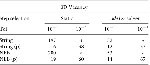
step selection, fitting thertolandatol parameter was simple as it was observed thatrtol= 0.1 was sufficient in most cases for conver-gence but other valuesrtol= 1 andrtol= 0.01 were occasionally more appropriate. The value ofatolwas chosen so thatatol/rtol= 1 in all cases except the 2D vacancy of Sec.IV A, whereatol/rtol= 0.01 had to be used instead.
A. Vacancy migration
First, we consider the diffusion of a vacancy in a two dimen-sional 60-atom triangular lattice governed by a Lennard-Jones potentialV(r) = 4𝜖[(σ/r)12−2(σ/r)6] with parameters𝜖= 1.0,σ=
2−1
6. The vacancy is located at the centre of the cell initially and
migrates in theydirection by one lattice spacing. Periodic boundary conditions are imposed in thexandydirections.Table Ishows the number of force calls per image required for convergence. The expo-nential preconditioner(Exp) introduced in Packwoodet al.12 with
parametersA= 3.0 andrcut= 2.5, which utilises bond-connectivity information to treat the ill-conditioning of the system allowed con-vergence beyond the 10−3 tolerance, which the unpreconditioned case could not achieve within a reasonable number of iterations. The latter came as a surprise to us as on the contrary to the real vacancy migration systems that we study next, this artificial setup exhibits more severe ill-conditioning. We note that for the unpreconditioned case when using theode12r time stepping for the string method, we had to useatol/rtol= 0.01. The absolute differences∥x1−x2∥∞
between the positions x1 andx2for the image nearest the saddle in converged paths with and without preconditioning, were of the order of 8×10⁻³.
Next, we considered a three dimensional system containing a vacancy, specifically a 107-atom Cu fcc supercell in a fixed cell with periodic boundary conditions. Interactions were modeled with a Morse potential with parametersA= 4.0,𝜖= 1.0 and the near-est neighbour distancer0= 2.55 Å with interactions between atoms expressed by V(r) =ϵ(e−2A(r/r0−1)−
2e−A(r/r0−1))
. The exponen-tial preconditioner introduced in Packwoodet al.12was used with
parametersA= 3.0 andrcut= 2.2r0= 5.62 Å.Table IIshows the num-ber of force evaluations per image needed for convergence to two preset tolerance limits. This example demonstrates how theode12r
[image:5.594.55.280.88.185.2]solver can aid the performance of the string and NEB methods if
TABLE I. Number of force evaluations per image required by the string and NEB methods to converge the vacancy migration MEP in a 9 image path of a 60-atom 2D cell modeled with a Lennard-Jones potential, with either the static orode12rstep length selection methods. In the cases marked∗, the algorithm did not converge
within a reasonable number of iterations.
2D Vacancy
Step selection Static ode12rsolver
Tol 10−1 10−3 10−1 10−3
String 197 ∗ 52 ∗
String (p) 16 38 12 33
NEB 200 ∗ 53 ∗
[image:5.594.307.553.580.688.2]TABLE II. Force evaluations per image needed for the string and NEB methods for the migration of a vacancy in a 107-atom Cu fcc supercell modeled by a Morse potential. The MEP was discretised with 5 images.
Vacancy in Cu supercell
Step selection Static ode12rsolver
Tol (eV/Å) 10−1 10−3 10−1 10−3
String 8 74 8 41
String (p) 7 38 8 21
NEB 8 57 8 27
NEB (p) 7 37 8 19
a static step is not suitable. Preconditioning gave almost a 2-fold speedup for the higher accuracy results but no improvement for the lower accuracy. The absolute differences of the positions of the con-verged paths at the saddle, as performed before, were well below 3×10⁻¹⁴Å.
A 53-atom W bcc supercell modeled with the EAM4 poten-tial described in Ref.20was examined as well. Periodic boundary conditions were imposed. Aforce field(FF)preconditionerwas con-structed by suitably modifying the EAM Hessian to enforce positiv-ity; see the work of Moneset al.13(p. 9) for full details. This yields
up to 6 times faster convergence for higher accuracies as shown in Table III. The absolute differences of the positions of the converged paths at the saddle were well below 5×10⁻⁹Å.
We studied the same 53-atom W vacancy system with den-sity functional theory (DFT) as implemented in the Castep21
soft-ware. The exchange correlation functional was approximated by the Perdew, Burke, and Ernzerhof (PBE) generalised gradient approxi-mation (GGA),22with a plane wave energy cutoff of 500 eV and a
[image:6.594.45.289.581.688.2]2×2×2 Monkhorst-Pack grid to sample the Brillouin zone (a com-parison of convergence behavior obtained with a 3×3×3 k-point grid was carried out which showed that the use of the 2×2×2 k-point grid is sufficient). Step selection withode12r step and static step selection schemes was studied. A regularised FF preconditioner based on the EAM Hessian was used,P= (1−λ)PFF+λPExp+cI,
TABLE III. Force evaluations per image needed for the string and NEB methods to converge the MEP for vacancy migration in a 53-atom W bcc supercell modeled by the EAM4 potential.20The path was discretised by 5 images, and the preconditioner was constructed from the force field.13
Vacancy in W supercell
Step selection Static ode12r solver
Tol (eV/Å) 10−1 10−3 10−1 10−3
String 7 77 7 49
String (p) 5 12 5 9
NEB 8 58 7 35
NEB (p) 5 10 8 17
wherec= 0.05,λ= 0.4,PFFis described in Ref.13, p. 9, and thePExp parameters were fitted toPFF.
The path is made up of 5 images, and traversing the path in subsequent iterations of the NEB and string methods was performed in an alternating order, allowing efficient reuse of previous electronic structure data to start the next optimisation step.
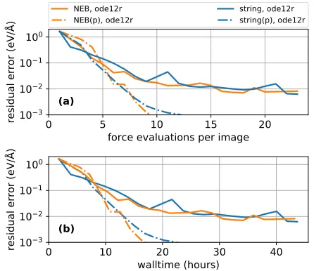
Unlike the EAM case above, the preconditioner we used for the DFT model does not describe the potential energy surface of the DFT model exactly but nevertheless gives a speed-up of a factor of two for an accuracy of∼10−2eV/Å and furthermore allows accuracies of the
order of∼10−3eV/Å to be achieved, unlike the unpreconditioned case, as shown inFigs. 2and3. The results ofTable IIIsuggest that constructing a better preconditioner would improve these results further. Notice further that the number of force evaluations needed for convergence and the time needed for convergence are in agree-ment (by comparison of the upper and lower panes ofFigs. 2and3), confirming that the computational cost of constructing the precon-ditioner model is negligible compared to the cost of computing DFT forces, justifying our earlier assumptions. We note that the gain of preconditioning would be expected to further increase with the sys-tem size.12The absolute differences of the positions of the converged
paths at the saddle were of the order of 1×10⁻⁴Å. B. Screw dislocation
In the final example, we study a 1
2⟨111⟩screw dislocation in a 562-atom W bcc structure confined in a cylinder of radius equal to 20 Å and surrounded by an 11 Å cylindrical shell of clamped atoms, with periodic boundary conditions along the dislocation line (z) direction. The system is simulated with the same EAM4 poten-tial. The dislocation advances by one glide step.Table IVshows the
FIG. 3. Convergence of the string and NEB methods with and without precondi-tioner for a 53-atom W bcc supercell containing a vacancy and modeled with DFT. The upper panel (a) shows the error as a function of the number of force evalua-tions per image and the lower panel (b) shows the error as a function of the time required to converge. The static time step was chosen by extrapolating theode12r
data. The path was discretised by 5 images.
computational costs for converging the MEP with the NEB and string methods, using either static orode12rstep length selection. A force field preconditioner built from the same EAM potential was used for geometry optimisation.
Upon preconditioning, we observed a 5-fold speed up for the static case for low accuracies but only a 2-fold speed up for the
[image:7.594.57.279.86.276.2]ode12rcase. For a higher accuracy, a speed up of a factor of 6 was observed and there was a speed up of a factor of at least 2 from using theode12rstep selection over the static step selection for both the unpreconditioned and preconditioned cases. This indicates that the fitted static step is only suitable in the pre-asymptotic regime and a larger step size is suitable in the asymptotic regime, showcasing the advantages of using the adaptiveode12rscheme over the hand-tuned static step. The absolute differences of the positions of the converged paths at the saddle were below 2×10⁻³Å.
TABLE IV. Computational cost for the NEB and string methods for a screw dislocation in a 562-atom W bcc cylinder simulated with the EAM4 Marinica potential.20The circular boundary is fixed at a radius of R = 20Å. Periodic boundary conditions were imposed in thezdirection. The path was discretised by 9 points.
Screw dislocation
Step selection Static ode12r solver
Tol (eV/Å) 10−1 10−3 10−1 10−3
String 40 272 14 124
String (p) 7 48 9 21
NEB 40 312 14 162
NEB (p) 7 47 7 21
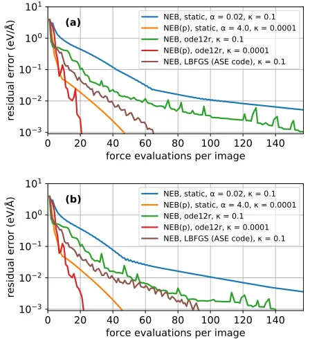
We investigated this system further, focusing on the NEB implementation to allow comparison with the widely used Limited memory Broyden—Fletcher—Goldfarb—Shanno (LBFGS)23
opti-misation algorithm, which can be used with the NEB implemen-tation10 in the Atomic Simulation Environment (ASE).24 This
required fixing the end points of the path at the minima as is per-formed in the ASE code. The comparison was carried out on sys-tems of two sizes. A force field preconditioner was used as before for the preconditioned cases.Figure 4shows the convergence rate of the various NEB schemes for a radius of 20 Å in the upper panel (a) and for a radius of 40 Å in the lower panel (b). Note that although LBFGS gave good convergence in the unprecondi-tioned case, it lacks robustness. This is because the force field of the NEB algorithm is not conservative, violating one of LBFGS’s assumptions. LBFGS constructs a Hessian matrix corresponding to a scalar field, failing to capture the effects of the transport terms of the NEB force field. Moreover, the lack of the energy function prevents the use of line search, required to ensure the method’s stability; in the ASE LBFGS implementation, a heuristic is instead used to impose a maximum step length of 0.04 Å. Furthermore, it should be noted that because our preconditioning scheme does not treat the longitudinal force components, it is inappropriate for
[image:7.594.317.541.342.587.2] [image:7.594.45.290.582.690.2]us to use it together with the LBFGS method for MEP finding methods.
V. CONCLUSIONS
We have demonstrated that MEP finding techniques such as the NEB and the string method can exhibit slow convergence rates due to poor search direction and step-length selection during the optimisation procedure. We have introduced a new optimisation technique combining an adaptive time-stepping scheme with pre-conditioning to address ill-pre-conditioning of the energy landscape in directions transverse to the path and to allow faster convergence to the minimum energy path.
We observed that our new scheme gives a significant speed up and improved robustness over currently used approaches for a range of systems using both force fields and DFT. Moreover, it allows higher accuracies to be reached than existing methods.
However, our preconditioning scheme targets transverse ill-conditioning only. The longitudinal terms (e.g., the NEB spring interactions) are unaffected by the preconditioner, suggesting that our scheme provides a baseline for further improvements.
An open source prototype implementation of our technique is available athttps://github.com/cortner/SaddleSearch.jl.
ACKNOWLEDGMENTS
This work was supported by the Engineering and Physical Sci-ences Research Council (EPSRC) under Grant Nos. EP/P002188/1, EP/R012474/1, EP/J021377/1, and EP/R043612/1, by ERC Start-ing Grant No. 335120, and by the Royal Society under Grant No. RG160691. Computing facilities were provided by the Scien-tific Computing Research Technology Platform of the University of Warwick with support from the Science Research Investment Fund. We thank Petr Grigorev for providing the screw dislocation configurations.
APPENDIX: REPARAMETERISING IN PRECONDITIONED STRING
The path reparameterisation described in Eq. (12) in Ref.7 assumes that the`2-metric is used to measure distance. Here, we briefly describe the modifications required when it is replaced with the metric dP defined in (8), used in the preconditioned string method introduced in Sec.III A.
After accepting an optimisation stepkof Eq.(7), the following steps are performed:
1. Compute the relative distances dP(xkn,xkn−1) between the images{xkn}n, for alln= 2,. . .,N.
2. Define
s1=0, sn= ∑
n
m=2dP(xkm,xkm−1)
∑N
m=2dP(xkm,xkm−1)
, forn=2,. . .,M. (A1)
3. Use cubic spline interpolation17of{s
n,xkn}Nn=1to obtainxk(s):
[0, 1] →RN.
4. The new images are then given by
xkn=xk(N−n−11), n=1,. . .,N. (A2) This algorithm doesnot ensure that images will be equidis-tributed according to dP. However it does ensure that images remain bounded away from one another, which is the key property required for the string method.
REFERENCES
1
A. F. Voter, F. Montalenti, and T. C. Germann,Annu. Rev. Mater. Res.32, 321 (2002).
2
H. Eyring,J. Comput. Phys.3, 107 (1935).
3
E. Pollak and P. Talkner,Chaos15, 026116 (2005).
4
G. H. Vineyard,J. Phys. Chem. Solids3, 121 (1957).
5
A. F. Voter,Radiation Effects in Solids, NATO Science Series Vol. 235 (Springer Netherlands, 2007), p. 1.
6
W. E, W. Ren, and E. Vanden-Eijnden,Phys. Rev. B66, 052301 (2002).
7
W. E, W. Ren, and E. Vanden-Eijnden,J. Chem. Phys.126, 164103 (2007).
8
M. Cameron, R. V. Kohn, and E. Vanden-Eijnden,J. Nonlinear Sci.21, 193 (2011).
9
H. Jónsson, G. Mills, and K. W. Jacobsen,Classical and Quantum Dynamics in Condensed Phase Simulations(World Scientific Publishing Co. Pte. Ltd., 1998), p. 385.
10
G. Henkelman and H. Jónsson,J. Chem. Phys.113, 9978 (2000).
11
J. Nocedal and S. J. Wright,Springer Series in Operations Research and Financial Engineering(Springer, Berlin, 2006).
12D. Packwood, J. Kermode, L. Mones, N. Bernstein, J. Woolley, N. Gould,
C. Ortner, and G. Csányi,J. Chem. Phys.144, 164109 (2016).
13
L. Mones, C. Ortner, and G. Csanyi,Sci. Rep.8, 13991 (2018).
14
R. Lindh, A. Bernhardsson, G. Karlström, and P.-Å. Malmqvist,Chem. Phys. Lett.241, 423 (1995).
15M. C. Payne, M. P. Teter, D. C. Allan, T. A. Arias, and J. D. Joannopoulos,Rev. Mod. Phys.64, 1045 (1992).
16
W. E and X. Zhou,Nonlinearity24, 1831 (2011).
17
P. Dierckx,Curve and Surface Fitting with Splines(Oxford University Press, Inc., New York, NY, USA, 1993).
18E. Hairer, S. P. Nørsett, and G. Wanner,Solving Ordinary Differential Equations I: Nonstiff Problems, 2nd rev. ed.(Springer-Verlag New York, Inc., New York, NY, USA, 1993).
19H. Lamba,BIT Numer. Math.40, 314 (2000).
20M.-C. Marinica, L. Ventelon, M. R. Gilbert, L. Proville, S. L. S. L. Dudarev,
J. Marian, G. Bencteux, and F. Willaime,J. Phys.: Condens. Matter25, 395502 (2013).
21S. Clark, M. Segall, C. Pickard, P. Hasnip, M. Probert, K. Refson, and M. Payne, Z. Kristallogr.–Cryst. Mater.220, 567 (2005).
22
J. P. Perdew, K. Burke, and M. Ernzerhof,Phys. Rev. Lett.77, 3865 (1996).
23
D. C. Liu and J. Nocedal,Math. Program.45, 503 (1989).
24
A. H. Larsen, J. J. Mortensen, J. Blomqvist, I. E. Castelli, R. Christensen, M. Dułak, J. Friis, M. N. Groves, B. Hammer, C. Hargus, E. D. Hermes, P. C. Jennings, P. B. Jensen, J. Kermode, J. R. Kitchin, E. L. Kolsbjerg, J. Kubal, K. Kaasbjerg, S. Lysgaard, J. B. Maronsson, T. Maxson, T. Olsen, L. Pastewka, A. Peterson, C. Rostgaard, J. Schiøtz, O. Schütt, M. Strange, K. S. Thygesen, T. Vegge, L. Vilhelmsen, M. Walter, Z. Zeng, and K. W. Jacobsen,J. Phys.: Condens. Matter