Judgmental Selection of Forecasting Models

(1)

Contents lists available atScienceDirect

Journal of Operations Management

journal homepage:www.elsevier.com/locate/jom

Judgmental selection of forecasting models

Fotios Petropoulos

a

, Nikolaos Kourentzes

b

, Konstantinos Nikolopoulos

c

, Enno Siemsen

d,∗ a_{School of Management, University of Bath, UK}

b_{Lancaster University Management School, Lancaster University, UK} c_{Bangor Business School, Bangor University, UK}

d_{Wisconsin School of Business, University of Wisconsin, USA}

A R T I C L E I N F O

Keywords: Model selection Behavioral operations Decomposition Combination

A B S T R A C T

In this paper, we explored how judgment can be used to improve the selection of a forecasting model. We compared the performance of judgmental model selection against a standard algorithm based on information criteria. We also examined the eﬃcacy of a judgmental model-build approach, in which experts were asked to decide on the existence of the structural components (trend and seasonality) of the time series instead of directly selecting a model from a choice set. Our behavioral study used data from almost 700 participants, including forecasting practitioners. The results from our experiment suggest that selecting models judgmentally results in performance that is on par, if not better, to that of algorithmic selection. Further, judgmental model selection helps to avoid the worst models more frequently compared to algorithmic selection. Finally, a simple combi-nation of the statistical and judgmental selections and judgmental aggregation signiﬁcantly outperform both statistical and judgmental selections.

1. Introduction

Planning processes in operations - e.g., capacity, production, in-ventory, and materials requirement plans - rely on a demand forecast. The quality of these plans depends on the accuracy of this forecast. This relationship is well documented (Gardner, 1990; Ritzman and King, 1993; Sanders and Graman, 2009; Oliva and Watson, 2009). Small improvements in forecast accuracy can lead to large reductions in in-ventory and increases in service levels. There is thus a long history of research in operations management that examines forecasting processes (Seifert et al., 2015;Nenova and May 2016;van der Laan et al., 2016, are recent examples).

Forecasting model selection has attracted considerable academic and practitioner attention during the last 30 years. There are many models to choose from – different forms of exponential smoothing, autoregressive integrated moving average (ARIMA) models, neural nets, etc.–and forecasters in practice have to select which one to use. Many academic studies have examined different statistical selection methodologies to identify the best model; the holy grail in forecasting research (Petropoulos et al., 2014). If the most appropriate model for each time series can be determined, forecasting accuracy can be sig-nificantly improved (Fildes, 2001), typically by as much as 25–30% (Fildes and Petropoulos, 2015).

In general, forecasting software recommends or selects a model

based on a statistical algorithm. The performance of candidate models is evaluated either on sample data, usually using appropriate in-formation criteria (Burnham and Anderson, 2002), or by withholding a set of data points to create a validation sample (out-of-sample evalua-tion,Ord et al., 2017, also known as cross-validated error). However, it is easy to devise examples in which statistical model selection (based either on in-sample or out-of-sample evaluation) fails. Such cases are common in real forecasting applications and thus make forecasting model selection a non-trivial task in practice.

Practitioners can apply judgment to diﬀerent tasks within the forecasting process, namely:

1. deﬁnition of a set of candidate models, 2. selection of a model,

3. parametrization of models, 4. production of forecasts, and 5. forecast revisions/adjustments.

Most of the attention in the judgmental forecasting literature fo-cuses on the latter two tasks. Experts are either asked to directly esti-mate the point forecasts of future values of an event or a time series (see for exampleHogarth and Makridakis, 1981;Petropoulos et al., 2017), or they are asked to adjust (or correct) the estimates provided by a statistical method in order to take additional information into account;

https://doi.org/10.1016/j.jom.2018.05.005

Received 3 October 2017; Received in revised form 22 May 2018; Accepted 23 May 2018

∗_{Corresponding author.}

E-mail address:[email protected](E. Siemsen).

(2)

such information is often called soft data, such as information from the sales team (Fildes et al., 2009).

However, little research has examined the role and importance of human judgment in the other three tasks. In particular, Bunn and Wright (1991)referred to the problem of judgmental model selection (item 2 in the above list), suggesting that the selection of the most appropriate model(s) can be based on human judgment. They also emphasized the dearth of research in this area. Importantly, the ma-jority of the world-leading forecasting support systems allow human judgment as theﬁnal arbiter among a set of possible models.1 Thefore, the lack of research into how well humans perform this task re-mains a substantive gap in the literature.

In this study, we examined how well human judgment performs in model selection compared with an algorithm using a large-scale beha-vioral experiment. We analyzed the efficiency of judgmental model selection of individuals as well as groups of participants. The frequency of selecting the best and worst models provides suggestions on the ef-ficacy of each approach. Moreover, we identified the process that most likely will choose models that lead to improved forecasting perfor-mance.

The rest of our paper is organized as follows. The next section provides an overview of the literature concerning model selection for forecasting. The design of the experiment to support the data collection is presented in section 3. Section4 shows the results of our study. Section 5 discusses the implications for theory, practice, and im-plementation. Finally, section6contains our conclusions.

2. Literature

2.1. Commonly used forecasting models

Business forecasting is commonly based on simple, univariate models. One of the most widely used families of models are exponential smoothing models. Thirty different models fall into this family (Hyndman et al., 2008). Exponential smoothing models are usually abbreviated as ETS, which stands for either ExponenTial Smoothing or Error, Trend, Seasonality (the three terms in such models). More spe-cifically, the error term may be either additive (A) or multiplicative (M), whereas trend and seasonality may be none (N), additive (A), or multiplicative (M). Also, the trend can be linear or damped (d). As an example, ETS(M,Ad,A) refers to an exponential smoothing model with a multiplicative error term, a damped additive trend, and additive sea-sonality. Maximum likelihood estimation is used to find model para-meters that produce optimal one-step-ahead in-sample predictions (Hyndman and Khandakar, 2008).

These models are widely used in practice. In a survey of forecasting practices, the exponential smoothing family of models is the most fre-quently used (Weller and Crone, 2012). In fact, it is used in almost 1/3 of times (32.1%), with averages coming second (28.1%) and naive methods third (15.4%). More advanced forecasting techniques are only used in 10% of cases. In general, simpler methods are used3/4times, a result that is consistent with the relative accuracy of such methods in forecasting competitions. Furthermore, an empirical study that eval-uated forecasting practices and judgmental adjustments reveals that “the most common approach to forecasting demand in support of supply chain planning involves the use of a statistical software system which incorporates a simple univariate forecasting method, such as exponential smoothing, to produce an initial forecast” (Fildes et al., 2009, p. 4), while it speciﬁes that three out of four companies examined “use systems that are based on variants of exponential smoothing” (Fildes et al., 2009, p. 7).

There are many alternatives to exponential smoothing for producing business forecasts, such as neural networks and other machine learning methods. Nevertheless, time series extrapolative methods remain very attractive. This is due to their proven track record in practice (Gardner, 2006) as well as their relative performance compared to more complex methods (Makridakis and Hibon, 2000;Armstrong, 2006;Crone et al., 2011). Furthermore, time series methods are fairly intuitive, which makes them easy to specify and use, and enhances their acceptance by the end-users (Dietvorst et al., 2015;Alvarado-Valencia et al., 2017). Complex methods, such as many machine learning algorithms, often appear as black boxes, and provide limited or no insights into how the forecasts are produced and which data elements are important. These attributes of forecasting are often critical for users (Sagaert et al., 2018).

2.2. Algorithmic model selection

Automatic algorithms for model selection are often built on in-formation criteria (Burnham and Anderson, 2002; Hyndman et al., 2002). Models within a certain family (such as exponential smoothing or ARIMA) arefitted to the data, and the model with the minimum value for a specific information criterion is selected as the best. Various information criteria have been considered, such as Akaike's Information Criterion (AIC) or the Bayesian Information Criterion (BIC). The AIC after correction for small sample sizes (AICc) is often recommended as the default option because it is an appropriate criterion for short time series and it differs only minimally from the conventional AIC for longer time series (Burnham and Anderson, 2002). However, research also suggests that if we focus solely on out-of-sample forecasting ac-curacy, the various information criteria may choose different models that nonetheless result in almost the same forecast accuracy (Billah et al., 2006).

Information criteria are based on the optimized likelihood function penalized by model complexity. Using a model with optimal likelihood inadvertently assumes that the postulated model is true (Xia and Tong, 2011). In a forecasting context, this assumption manifests itself as fol-lows: The likelihood approach generally optimizes the one-step-ahead errors; for the forecasts to be optimal for multi-step ahead forecasts, the resulting model parameters should be optimal for any longer horizon error distribution as well. This will only occur if the model is true, in which case the model fully describes the structure of the series. Otherwise, the error distributions will vary with the time horizon (Chatﬁeld, 2000). Such time-horizon dependent error distributions are often observed in reality (Barrow and Kourentzes, 2016), providing evidence that any model merely approximates the underlying unknown true process. Not recognizing this can lead to a biased model selection which favors one-step-ahead performance at the expense of longer time horizons that may well be the analyst's real objective.

An alternative to selecting models via information criteria is to measure the performance of different models in a validation set (Fildes and Petropoulos, 2015;Ord et al., 2017). The available data are divided intofitting and validation sets. Models arefitted using thefirst set, and their performance is evaluated in the second set. The model with the best performance in the validation set is put forward to produce fore-casts for the future. The decision maker can choose the appropriate accuracy measure. The preferred measure can directly match the actual cost function that is used to evaluate thefinal forecasts.

Forecasts for validation purposes may be produced only once (also known as ﬁxed-origin validation) or multiple times (rolling-origin), which is the cross-validation equivalent for time series data. Evaluating forecasts over multiple origins has several advantages, most im-portantly their robustness against the peculiarities in data that may appear within a single validation window (Tashman, 2000). Model selection on (cross-)validation has two advantages over selection based on information criteria. First, the performance of multiple-step-ahead forecasts can be used to inform selection. Second, the validation 1_{For example, see the}_{‘Manual Model Selection’}_{feature of SAP Advanced Planning and}

Optimization (SAP APO), on SAP ERP: https://help.sap.com/viewer/ c95f1f0dcd9549628efa8d7d653da63e/7.0.4/en-US/

(3)

approach is able to evaluate forecasts derived from any process (in-cluding combinations of forecasts from various models). The dis-advantage of this approach is that it requires setting aside a validation set, which may not always be feasible. Given that product life cycles are shortening, having a validation sample available can be an out of reach luxury for forecasters.

Aﬁnal category for automatic model selection involves measure-ment of various time series characteristics (such as trend, seasonality, randomness, skewness, intermittence, variability, number of available observations) as well as consideration of decision variables (such as the forecast horizon). Appropriate models are selected based on expert rules (Collopy and Armstrong, 1992; Adya et al., 2001) or meta-learning procedures (Wang et al., 2009; Petropoulos et al., 2014). However, such approaches are very sensitive to the selected rules or meta-learning features. No widely accepted set of such rules exists.

Regardless of the approach used for theautomaticselection of the best model, all processes outlined above (information criteria, valida-tion, and selecting based on rules) are based on statistics or can be implemented through an algorithmic process. A commonality among all algorithmic model selection approaches is that selection is based on historical data. None of these algorithms can evaluate forecasts when the corresponding actual values (for example, actually realized de-mand) are not yet available. These statistical selection approaches have been adopted from non-time series modeling problems in which the predictive aspect of a model may not be present. Therefore, forecasting is only implicitly accounted for in these algorithmic approaches. Good forecasts, rather than good descriptions of the series, are done with a “leap of faith”.

2.3. Model selection and judgment

Despite the fact that the automatic selection of forecasting models has been part of many statistical packages and commercial software, what is often observed in practice is that managers select a model (and in some cases parameters) in a judgmentalway. Automatic selection procedures are often hard to understand and communicate within companies. In that sense, managers lack trust in automatic statistical forecasting (Alvarado-Valencia et al., 2017). A standard issue is that automatic selection methods tend to change models between successive planning periods, substantially altering the shape of the series of fore-casts. This issue reduces the users' trust in the system, especially after the statistical selection makes some poor choices (Dietvorst et al., 2015). Users then eventually resort to either fully overriding the sta-tistical selection or implementing custom ad-hoc judgmental “ correc-tion”rules.

Moreover, managers often believe ﬁrmly that they better under-stand the data and the business context that created the data. For ex-ample, even if the result of an algorithm suggests that the data lacks any apparent seasonality (and as such a seasonal model would not be ap-propriate), managers may still manually select a seasonal model be-cause they believe that this better represents the reality of their busi-ness. Lastly, the sense of ownership of forecasts can drive experts to override statistical results because more often than not evaluation of their work performance is associated with taking actions about the forecasts (Önkal and Gönül, 2005;Ord et al., 2017), or is inﬂuenced by organizational politics (Kolassa and Siemsen, 2016;Ord et al., 2017).

To the best of our knowledge, the efficacy of judgmental model selection has not been studied. We expect that when forecast models are presented in a graphical environment (actual data versusfitted values plus forecasts, as is the case in the majority of forecasting software), forecasters may pay little attention to the actualfit of the model in the in-sample data (or the respective value of the AIC if provided). However, critical to the judgmental selection will be the matching of the out-of-sample forecasts with the expected reality. Harvey (1995) observed that participants in a laboratory experiment made predictions so that the noise and patterns in the forecasts were representative of the

past data. Thisﬁnding leads us to believe that forecasters perform a mental extrapolation of the available in-sample data, rejecting the models that result in seemingly unreasonable forecasts and accepting the ones that represent a possible reality for them. Thus, in contrast to algorithmic model selection, forecasters will attempt to evaluate the out-of-sample forecasts, even if the future realized values of the fore-casted variable are not yet available.

As the amount of information increases, decision makers are unable to process it efficiently and simultaneously (Payne, 1976). Accordingly, research in decision analysis and management judgment has estab-lished that decomposition methods, which divide a task into smaller and simpler ones, lead to better judgment. Such methods have also been found to be useful in judgmental forecasting tasks, especially for fore-casts that involve trends, seasonality and/or the effect of special events such as promotions.Edmundson (1990)examined the performance of judgmental forecasting under decomposition. Similar to the way ex-ponential smoothing works (Gardner, 2006), forecasters were asked to estimate the structural components of the time series (level, trend, and seasonality) separately. The three estimates were subsequently com-bined (Edmundson, 1990). found that estimating the components in-dependently resulted in superior performance compared with produ-cing judgmental forecasts directly. In another study, Webby et al. (2005)observed similar results when the effects of special events were estimated separately. Also,Lee and Siemsen (2017)demonstrated the value of task decomposition on order decisions, especially when cou-pled with decision support.

We expect that these insights may be applied to judgmental model selection. When judgmentally selecting between forecasting models (through a graphical interface), we expect a model-build approach to outperform the simple choice between diﬀerent models. In a model-build approach, forecasters are asked to verify the existence (or not) of structural components (trend and seasonality). This changes the task from identifying the best extrapolation line to determining whether the historical information exhibits speciﬁc features that the expert believes will extend into the future.

2.4. Combination and aggregation

Forecast combinations can result in significant improvement in forecast accuracy (Armstrong, 2001). There is also ample evidence that combining the output of algorithms with the output of human judgment can confer benefits.Blattberg and Hoch (1990)used a simple (50-50%) combination and found significant gains in combination methods compared with the separate use of algorithms and judgment. Their results have been repeatedly confirmed in the forecasting literature. Franses and Legerstee (2011) found that a simple combination of forecasts outperformed both statistical and judgmentally adjusted forecasts.Petropoulos et al. (2016)demonstrated that a 50-50 combi-nation of forecasts in the period after a manager's adjustments have resulted in significant losses can indeed increase accuracy by 14%. Wang and Petropoulos (2016)found that a combination is as good, if not better, than selecting between a statistical or an expert forecast. Trapero et al. (2013)demonstrated further gains with more complex combination schemes. We anticipate that a combination will also be beneficial in the context of forecast model selection.

(4)

judgmental model selections will lead to improved performance com-pared with selecting a single model, either judgmentally or statistically.

3. Design of the behavioral experiment

3.1. Selecting models judgmentally

Specialized forecasting software lists forecast methods and models. The users of such systems must choose one from the list to extrapolate the data at hand. In some cases, this list of choices is complemented by an option that, based on an algorithm, automatically identifies and applies the best of the available methods. However, in the context of the current paper, we assumed that forecasters do not have such a re-commendation available and instead rely solely on their own judgment. We also assumed that the choice set is constrained to four models able to capture various data patterns (level, trend, and seasonality). This is not an unreasonable setup, with some established systems offering such specific options (such as the well established SAP APO-DP system). We resorted to the exponential smoothing family of models (Hyndman et al., 2008) and focused on the four models presented in Table 1 (mathematical expressions are provided inAppendix A).

To emulate the simple scenario implied by standard forecasting support systems (choose one of the available forecasting models), we used radio buttons to present the diﬀerent model-choices as a list, as depicted in the left part ofFig. 1. A user can navigate across the dif-ferent choices and examine the forecasts produced by each method. Once the forecasts produced by a method are considered satisfactory, then a manager can submit the choice and move to the next time series. We call this approach“judgmental model selection”.

We also considered a second approach where the user builds a model instead of selecting between models. In the“model-build” con-dition, we ask a user to identify the existence of a trend and/or sea-sonality in the data; the response can be used to select the respective

model from theTable 1. For example, identification of a trend implies damped exponential smoothing; identification of seasonality without a trend implies SES with seasonality. This can be implemented in the software design by including two check-boxes (right panel ofFig. 1). Once a change in one of these two check-boxes has been made, the forecasts of the respective model are drawn. To facilitate identification, we provide trend and seasonal plots (with usage instructions) in an attempt to aid the users with the pattern identification task.

In both cases, once a participant submits his or her decisions, we use the selected forecasting method to produce one-year-ahead (12 months) forecasts for that time series. The forecasts are compared with the ac-tual future values, which were withheld, toﬁnd the forecast accuracy of the submitted choice.

3.2. Data

To compare the performance of statistical versus judgmental model selection, we used a subset of time series from the M3-Competition dataset (Makridakis and Hibon, 2000). This dataset consists of 3003 real time series of various frequencies and types. It has been used many times in empirical evaluations of new forecasting models or processes (Hyndman et al., 2002;Taylor, 2003;Hibon and Evgeniou, 2005;Crone et al., 2011;Athanasopoulos et al., 2017;Petropoulos et al., 2018). We did not disclose the data source to the participants.

We focused on series with a monthly frequency and handpicked 32 time series. We selected series so that in half of them, the statistical model selection based on minimizing the value of the AIC succeeds in identifying the best model as evaluated in the hold-out sample (out-of-sample observations). For the other half, this minimum-AIC model fails to produce the best out-of-sample forecast. Moreover, the 32 time series were selected so that all four exponential smoothing models considered in this paper (Table 1) are identiﬁed as best in some time series ac-cording to the AIC criterion.

[image:4.595.36.289.78.138.2]

This success rate of 50% for the statistical algorithm to pick the correct model probably overestimated (but not by much) the true success rate. When the four models presented in section3.1were ap-plied on the 1428 monthly series of the M3-competition, selection based on AIC is accurate in 36% of the cases. As such, if any bias is introduced by our time series selection, we favor the statistical algo-rithm by giving the algoalgo-rithm a higher chance of picking the correct model. Consequently, the true eﬀect size with which human judgment improves upon performance may be underestimated in our analysis. Table 1

The four forecasting models considered in this study.

Model description ETS Model Trend Seasonality

Simple exponential smoothing (SES) A,N,N ✗ ✗ SES with additive seasonality A,N,A ✗ ✓

Damped exponential smoothing (DES) A,Ad,N ✓ ✗ DES with additive seasonality A,Ad,A ✓ ✓

[image:4.595.65.531.508.716.2]

(5)

Because time series from the M3-Competition are of various lengths, we truncated all selected series to a history of 72 months (six years). Thefirstfive years of data (60 months) were treated as the in-sample data, on which the models werefitted. The last year (12 months) was used for out-of-sample evaluation.Fig. 2depicts a typical time series used in this behavioral experiment. Along with the historical data that coverfive years, we also draw the (unobserved) future of the series. Moreover, we show the statistical point forecasts of the four ex-ponential smoothing models considered in different colors. For this example, the AIC method identifies the ETS(A,Ad,A) model as best and, in fact, produced the best out-of-sample forecasts.

3.3. Participants

The behavioral experiment was introduced as an elective exercise to groups of undergraduate and postgraduate students studying at various universities (Institutions with at least 20 participants include Bangor University, Cardiﬀ University, Lancaster University, the National Technical University of Athens, and Universidad de Castilla-La Mancha). Details regarding the modules where the experiment was introduced as an elective exercise are provided in table B.6 ofAppendix B. We ran the exercise as a seminar (workshop) session during the re-spective modules. The experiment was also posted to several relevant groups on LinkedIn and three major forecasting blogs. As an incentive, the participants were told they would receive £50 if their performance ranked within the top-20 across all the participants (seeLacetera et al., 2014, for some positive eﬀects in rewarding volunteers).

We recruited more than 900 participants; 693 of them completed the task. Upon commencing the task, the participants were asked to self-describe themselves as undergraduate/postgraduate students, re-searchers, practitioners, or other. At the same time, each participant was randomly assigned to either the“model selection”or“model-build” condition.Table 2presents the distribution of participants across roles (rows) and experimental conditions (columns).

Most previous behavioral studies of judgmental forecasting were limited to students' participation (Lee et al., 2007; Thomson et al., 2013), which is common in behavioral experiments (Deck and Smith, 2013). In this study, our sample of student participants was com-plemented by a sample of practitioners (90 forecasting experts). Prac-titioner participants come from a variety of industries, as depicted in table B.7 ofAppendix B. Our analysis also considered this sub-sample separately to check for diﬀerences and similarities between the prac-titioners and the students.

The completion rate was high for student participants (at 83%). This was expected, as the experiment was conducted in a lab for several cohorts of this population. The rate was lower for the other groups (practitioners 67%, researchers 57%, and other participants 56%). These observed completion rates are slightly lower than other profes-sional web-based surveys (78.6%2_{); this diﬀerence may be explained by} the duration of this behavioral experiment (around 30 min, as opposed to the recommended 15 min3_).

3.4. The process of the experiment

After being randomly assigned to experimental conditions, partici-pants were given a short description of the experimental task. The participants assigned to the model-build condition were given brief descriptions of the trend and seasonal plots.

The 32 time series we selected from the M3 Competition were di-vided into four groups of 8 time series each (the same for all partici-pants), and the actual experiment consisted of 4 rounds. In each round, the participants were provided with different information regarding the forecasts and thefit derived from each model. The purpose was to in-vestigate how different designs and information affect judgmental model selection or model-build. The information provided in each round is as follows:

•

Only the out-of-sample forecasts (point forecasts for the next 12 months) were provided.

•

The out-of-sample forecasts and the in-sample forecasts (modelﬁt) were provided.

•

The out-of-sample forecasts and the value of the AIC, which refers to theﬁt of the model penalized by the number of parameters, were provided.

[image:5.595.146.456.62.236.2] [image:5.595.37.288.667.743.2]

•

The out-of-sample forecasts, the in-sample forecasts, and the value Fig. 2.A typical time series used in this research, along with the forecasts from the four models.

Table 2

Participants per role and experiment.

Role Model Selection Model-Build Total

UG students 139 137 276

PG students 103 108 211

Researchers 13 31 44

Practitioners 46 44 90

Other 40 32 72

(6)

of the AIC were provided.

The order of the rounds, as well as the order of the time series within each round, was randomized for each participant. Attention checks (Abbey and Meloy, 2017) were not performed. To maximize participant attention, round-speciﬁc instructions were given at the be-ginning of each round so that the participants were able to identify and potentially use the information provided.

Our experiment has both a between-subjects factor (model selection vs. model-build) as well as a within-subjects factor (information pro-vided). Since the latter produced little meaningful variation, our ana-lysis focuses on the former. We chose this design since we believed that the difference between model selection vs. model-build could introduce significant sequence effects (making this more suited for between-sub-jects analysis), but we did not believe that differences in information provided would lead to sequence effects (making this more suited for within-subjects analysis).

3.5. Measuring forecasting performance

The performance of both algorithmic (based on AIC) and judg-mental model selection is measured on the out-of-sample data (12 monthly observations) that were kept hidden during the process of fitting the models and calculating the AIC values. Four metrics were used to this end. Thefirst metric was apercentage scorebased on the ranking of the selections. This was calculated as follows: A participant receives 3 points for the best choice (the model that leads to the best forecasts) for a time series, 2 points for the second best choice, and 1 point for the third best choice. Zero points were awarded for the worst (out of four) choices. The same point scheme can be applied to both judgmental forecasting approaches (model selection and model-build) once the identified patterns are translated to the respective model. The mean absolute error (MAE) was used as the cost function for evalua-tion. The range of points that anyone could collect is (given the number of time series) 0–96, which was then standardized to the more intuitive scale of 0–100. Thepercentage scoreof each participant, along with a pie chart presenting the distribution of best, second best, third best, and worst selections, was presented at the very last page of the experiment. Apart from the percentage score based on the selections, we also use three formal measures of forecasting performance: (1) Mean Percentage Error (MPE) is a measure suitable for measuring any systematic bias in the forecasts, (2) Mean Absolute Percentage Error (MAPE) and (3) Mean Absolute Scaled Error (MASE;Hyndman and Koehler, 2006) are suitable for measuring the accuracy of the forecasts. Although the MAPEsuffers from several drawbacks (Goodwin and Lawton, 1999), it is intuitive, easy to interpret, and widely used in practice.MASEis the

Mean Absolute Error scaled by the in-sample Mean Absolute Error of the naive method that uses the last observed value as a forecast. The intuition behind this scaling factor is that it can always be defined and only requires the assumption that the time series has no more than one unit root, which is almost generally true for real time series. Other scaling factors, such as the historical mean, impose additional as-sumptions, such as stationarity.MASEhas desirable statistical proper-ties and is popular in the literature. In particular,MASE is scale in-dependent without having the computational issues of MAPE. It is always defined andfinite, with the only exception being the extreme case where all historical data would be equal. Note that MAE and MASEwould both give the same rankings of the models within a series and, as a result, the samepercentage scores. However,MAE is a scale-dependent error measure and not suitable for summarizing across series. For all three measures,MPE,MAPE, andMASE, values closer to zero are better. Moreover, whereasMPE can take both positive and negative values, the values forMAPE andMASE are always non-ne-gative.

The values ofMPE,MAPE, andMASEfor a single time series across forecast horizons are calculated as

∑

= −

=

+ +

+

MPE H

H y f y

100

,

i

n i n i

n i

1

∑

= −

=

+ +

+

MAPE H

H y f y

100

,

i

n i n i

n i

1

= − ∑ −

∑ −

= + +

= −

MASE n y f

H y y

( 1)

,

i H

n i n i

j n

j j

1

2 1

whereytandftrefer to the actual and the forecasted value at periodt,n is the size of the training sample, andHis the forecast horizon.

4. Analysis

4.1. Individuals' performance

We next examined the performance of the judgmental model se-lection and judgmental model-build approaches. We contrasted their performance with the algorithmic model selection by AIC (Hyndman and Khandakar, 2008).

[image:6.595.68.529.556.730.2]

How do judgmental model selection and judgmental model-build perform based on the percentage score?The left panel ofFig. 3presents the centage scores of the participants under the two approaches. The per-formance of each participant is depicted with a dot marker (blue for the

(7)

practitioner participants, gray for all other participants), and the re-spective box-plots are also drawn. The square symbol represents the arithmetic mean of the percentage score for each approach. The hor-izontal (red) dashed line refers to the statistical benchmark (perfor-mance of automatic model selection based on AIC). Generally, partici-pants performed better under the model-build approach than the model selection approach. In essence, the average participant in model-build performs as well as the participant in the 75tthpercentile of the model selection approach. More importantly, participants under the model-build approach perform on average as well as the statistical selection. However, the diﬀerences in scores between individuals are large, with the range spanning between 32% and 83%.

Do humans select similarly to the algorithm? The middle and right panels ofFig. 3present, respectively, how many times the participants selected the best, second best, third best, and worst models under the model selection and model-build approaches. The differences in per-formance (in terms of percentage scores) between model selection and model-build derives from the fact that model-build participants were able to identify the best model more frequently. By comparing how frequently algorithms (red squares) and humans make the best and worst model selection, we can observe that humans are superior to algorithms in avoiding the worst model, especially in the model-build case. The differences are statistically significant according tot-tests for both best and worst selections and both strategies, model selection and model-build (p<0.01). The frequencies that algorithms and humans selected each model are presented in Table 3, along with how many times each model performs best in the out-of-sample data. We observe that algorithms generally select the level models (SES and SES with seasonality) more often compared to their trended counterparts. AIC, as with other information criteria, attempts to balance the goodness-of-fit of the model and its complexity as captured by the number of para-meters. More uniform distributions are observed for human selection and out-of-sample performance.

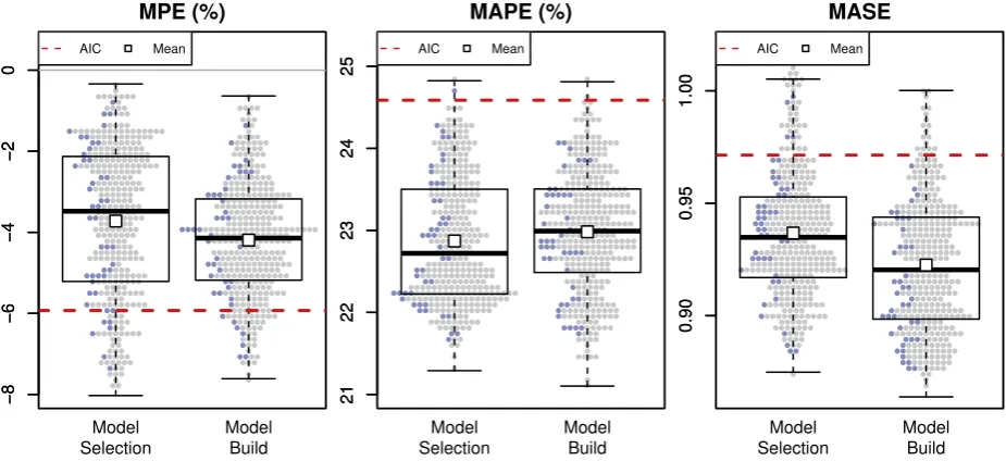
How do the judgmental approaches perform based on error measures? Fig. 4presents the performance of all 693 participants forMPE,MAPE, andMASE, the three error measures considered in this study. In both the model selection and the model-build treatments, human judgment is significantly better (less biased and more accurate) than statistical selection in terms ofMPEandMAPE. At the same time, although the judgmental model-build performs on a par with statistical selection for MASE, the judgmental model selection performs worse than the sta-tistical selection. Differences in the insights provided by the different error measures can be attributed to their statistical properties.

It is noteworthy that statistical selection is, on average, positively biased (negative values forMPE). However, this is not the case for all participants. In fact, slightly more than 30% of all participants (42% of those that were assigned in the model selection experiment) are, on average, negatively biased. The positive bias of statistical methods is consistent with the results ofKourentzes et al. (2014)who investigated the performance of statistical methods on all M3-competition data.

Do the results diﬀer if only the practitioners' subgroup is analyzed?

Independent sample t-tests were performed to compare the perfor-mance of practitioners and students. The results showed that differ-ences are not statistically significant, apart from the case of model-build andMASEwhere practitioner participants perform significantly better. The similarities in the results between student and practitioner

participants are relevant for the discussion of the external validity of behavioral experiments using students (Deck and Smith, 2013). Similar toKremer et al. (2015), our results suggest that student samples may be used for (at least) forecasting behavioral experiments.

4.2. Eﬀects of individuals' skill and time series properties

Going beyond the descriptives presented thus far, we constructed a linear mixed effects model to account for the variability in the skills of individual participants, as well as for the properties of each time series that was used. We model values ofMASE(containing the performance of the participants on each individual response: 693 participants×32 time series) considering the following fixed effects: (i) experimental condition (model selection or model-build); (ii) interface information (out-of-sample only, in- and out-of-sample and these options supple-mented with fit statistics; see section3.4); and (iii) the role of the participants (seeTable 2in which both under- and postgraduate stu-dents were grouped together). We accounted for the variation between participants as a random effect that reflects any variability in skill. Si-milarly, we consider the variability between time series as a second random effect, given that they have varying properties.

To conduct the analysis we use the lme4 package (Bates et al., 2015) for R statistical computing language (R Core Team, 2016). We eval-uated the contribution of each variable in model by using two in-formation criteria (AIC and BIC). To facilitate the comparison of the alternative model speciﬁcation using information criteria, we estimated the model using maximum likelihood. We found only marginal diﬀer-ences between the models recommended by the two criteria, a result suggesting that the most parsimonious option was the better choice.

We concluded that only the effect of the experimental condition was important, and that the interface information and role of participant did not explain enough variability to justify the increased model com-plexity. Consequently, these two effects were removed from the model. Both random effects were deemed useful. We investigated for random slopes as well, but found that such slopes did not explain any additional variability inMASE. Therefore, they were not considered further.

The resulting fully crossed random intercept model is reported in Table 4. The estimated model indicates that model-build improves MASEby 0.0496 over model select, which is consistent with the ana-lysis so far. The standard deviations of the participant and series eﬀects, respectively, are 0.0314 and 0.5551 (the intraclass correlations are 0.0026 and 0.8178). This shows that the skills of the participants ac-count for only a small degree of the variability ofMASE. This helps explain the insigniﬁcant role of the participant background. To put these values into perspective, the standard deviation ofMASE on in-dividual time series responses is 0.6144.

4.3. 50% statistics+50% judgment

The seminal work by Blattberg and Hoch (1990) suggested that combining the outputs of statistical models with managerial judgment will provide more accurate outputs than each single-source approach (modelormanager), while a 50-50% combination is“a nonoptimal but pragmatic solution”(Blattberg and Hoch, 1990, p. 898). Their result has been conﬁrmed in many subsequent studies. In this study, we considered the simple average of the two predictions, i.e., the equal-weight combination of the forecasts produced by the model selected by the statistics (AIC) and the model chosen by each participant.

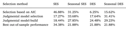
[image:7.595.38.288.676.735.2]

How does a 50-50 combination of statistical and judgmental selection perform?Fig. 5presents the performance of the simple combination of statistical and judgmental selection for the three error measures con-sidered in this study and categorized by the two judgmental approaches. We observed that performance for both judgmental model selection and model-build was improved signiﬁcantly compared with using statistical selection alone (horizontal dashed red line). In fact, the combination of the statistical+judgmental selection is less biased than statistical selection in Table 3

Frequencies of selected models.

Selection method SES Seasonal SES DES Seasonal DES

(8)

86% of the cases and produces lower values forMAPEandMASEfor 99% and 90% of the cases, respectively. Moreover, the diﬀerences in the per-formance of the two approaches are now minimized.

Does a 50-50 combination bring robustness?On top of the improve-ments in performance, an equal-weight combination also reduces the between-subject variation in performance. Focusing, for instance, on MASE and the judgmental model-build approach, Fig. 4 suggests a range of 0.314 (between 0.882 and 1.196) between best and worst performers. The comparable range according toFig. 5 is 0.136 (be-tween 0.864 and 1). Therefore, a 50-50 combination renders the judgmental selection approaches more robust.

4.4. Wisdom of crowds

An alternative to combining the statistical and judgmental selec-tions is judgmental aggregation–a combination of the judgmental se-lections of multiple participants. The concept of the “wisdom of crowds”is not new (Surowiecki, 2005) and has repeatedly been shown to improve forecast accuracy as well as the quality of judgments in general.

[image:8.595.64.529.59.274.2] [image:8.595.38.288.325.454.2]

For example, consider that a group of 10 experts is randomly se-lected. Given their selections regarding the best model, we can derive Fig. 4.Performance of model selection and model-build in terms of error measures when all participants are considered.

Table 4

Linear mixed eﬀects model output.

Mixed eﬀect model statistics

Fixed eﬀects

Estimate Standard Error Intercept 1.0313 0.0982 Experiment setup −0.0496 0.0042 Random eﬀects

Standard Deviation Participant (intercept) 0.0314

Time series (intercept) 0.5551 Residual 0.2601 Model statistics

AIC BIC Log Likelihood 3742.3 3782.3 −1866.1

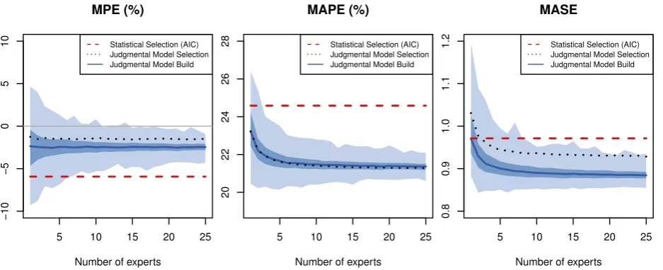
[image:8.595.65.528.517.729.2]

(9)

the frequencies that show how many times each model is identiﬁed as best. In other words, experts preferences are equally considered (each expert has exactly one vote, and all votes carry the same weight). This procedure leads to a weighted combination of the four models for which the performance can be measured. We consider groups of 1–25 experts randomly re-sampled 1000 times.

Does judgmental aggregation improve forecasting performance?Fig. 6 presents the results of judgmental aggregation. The light blue area describes the range of the performance of judgmental aggregation for various group sizes when the model-build approach is considered. The middle-shaded blue area refers to the 50% range of performances, and the dark blue line refers to the median performance. In other words, if one considers a vertical line (i.e., for particular group size), the points at which this line intersects provide the minimum,first quartile, median, third quartile, and maximum descriptive summary of the performance. For the judgmental model selection approach, only the median is drawn in the black dotted line, and the performance of statistical selection is represented by a red dashed horizontal line. We observed significant gains in performance as the group size increased, coupled with lower variance in the performance of different equally sized groups. We also observed the convergence of performance, meaning that no further gains were noticed in the average performance for group sizes higher than 20. Judgmental aggregation outperforms both statistical and in-dividual selection.

How many experts are enough?A careful examination of Fig. 6 re-veals, on top of the improvements if aggregation is to be used, the critical thresholds for deciding on the optimal number of experts in groups. We observed that if groups offive participants are considered, then their forecasting performance was almost always better than that of the statistical selection on all three measures, regardless of their role (undergraduate/postgraduate students, practitioners, researchers, or other). Of even more interest, the third quartile of groups of size two always outperforms the statistical benchmark. It is not thefirst time that the thresholds of two andfive appear in the literature. These results confirm previousfindings:“only two tofive individuals' forecasts must be included to achieve much of the total improvement”(Ashton and Ashton, 1985, p. 1499). This result holds even if we only consider specific sub-populations of our sample, e.g. practitioners only. Once judgmental aggregation is used, the results from practitioners are all-but identical to results from students and other participants.

Note that in this study we consider only unweighted combinations of the judgmental model selections. If the same exercise were carried dynamically (over time), then one could also consider, based on past performance, weighted combinations that have been proven to enhance

performance in other forecasting tasks (Tetlock and Gardner, 2015).

How does the model with the most votes perform? Instead of con-sidering a weighted-combination forecast based on votes across the four models, we have also examined a case in which the aggregate selection is the model with the most votes. In case two (or more) models are tied forﬁrst place in votes, then an equal-weight combination among them was calculated. The performance of this strategy is worse, in terms of the accuracy measures considered, than the wisdom of crowds with weighted combinations; moreover, the quality of the performance de-pends heavily on the sample selected (the variance is high even for groups with a large number of experts). However, on average, merely choosing the most-popular model still outperforms statistical selection.

[image:9.595.65.534.68.259.2]

4.5. Evaluation summary and discussion

Table 5summarizes the results presented in the above sections. As a sanity check, we also provide the performance of four additional sta-tistical benchmarks:

•

Random selectionrefers to a performance obtained by randomly se-lecting one of the four available choices. We have reported the ar-ithmetic mean performance when such a procedure is repeated 1000 times for each series. This benchmark is included to validate the choice of the time series and to demonstrate that non-random se-lection is indeed meaningful (in either a statistical or a judgmental manner).

[image:9.595.306.558.615.744.2]

•

Equal-weight combinationrefers to the simple average of the forecasts Fig. 6.Wisdom of crowds' performance for diﬀerent numbers of experts.

Table 5

Summary of the results; top-method is underlined; top-three methods are in boldface.

Method MPE (%) MAPE (%) MASE

Individual selection

Random selection −2.91 24.52 1.104 Selection based on AIC −5.93 24.59 0.971 Judgmental model selection −1.52 23.48 1.031 Judgmental model-build −2.45 23.30 0.982

Combination

Equal-weight combination −2.90 21.96 0.985 Weighted combination based on AIC −4.84 23.39 0.931 Combination of best two based on AIC −4.65 23.12 0.921

50-50% combination of AIC and judgment −3.96 22.93 0.930

(10)

across all four models. In other words, each model was assigned a weight of one-quarter. It is included as a benchmark of the perfor-mance of 50-50 combinations and the wisdom of crowds.

•

Weighted combinations based on AICwere proposed byBurnham and Anderson (2002)and evaluated byKolassa (2011). This approach showed improved performance over selecting the model with the lowest AIC. It is used in this study as a more sophisticated bench-mark for the wisdom of crowds.

•

Combination of best two based on AIC refers to the equal-weight combination of the best and second-best models based on the AIC values.

Focusing on theﬁrst four rows ofTable 5that refer to selecting a single model with diﬀerent approaches, random selection performs poorly compared with all other approaches. This is especially true in terms of MASE. Moreover, although it seems to be less biased than statistical selection, random selection's absolute value ofMPEis larger than any of the two judgmental approaches.

The lastﬁve rows ofTable 5present the performance of the various combination approaches. First, we observe that the equal-weight combination performs very well according to all metrics, apart from MASE. A weighted combination based on AIC improves the perfor-mance of the statistical benchmark, conﬁrming the results byKolassa (2011); however, it is always outperformed by both 50-50 combina-tions of statistical and judgmental selection and by the wisdom of crowds. Combination of the best two models based on AIC performs slightly better than weighted combination based on AIC.

We also present in boldface the top three performers for each me-tric. The top performer is underlined. We observe that the wisdom of crowds (which is based on model-build) is always within the top three and rankedﬁrst for two of the metrics. The wisdom of crowds based on model selection also performs on par. We believe that this is an exciting result because it demonstrates that using experts to select the appro-priate method performs best against state-of-the-art benchmarks.

5. Implications for theory, practice, and implementation

This work provides a framework for judgmental forecasting model selection, and highlights the conditions for achieving maximal gains. We now discuss the implications of our work for theory and practice as well as issues of implementation.

Statistical model selection has been dominated by goodness-of-fit derived approaches, such as information criteria, and by others based on cross-validated errors (Fildes and Petropoulos, 2015). Thefindings of our research challenge these approaches and suggest that an alter-native approach based on human judgment is feasible and performs well. Eliciting how experts perform the selection of forecasts may yield still more novel approaches to statistical model selection. Our research provides evidence that a model-build approach works better for hu-mans. We postulate that model-build implies a suitable structure (and a set of restrictions) that aid selection. Statistical procedures could po-tentially benefit from a similar framing.

Our ﬁndings are aligned with the literature on judgmental fore-casting as well as research in behavioral operations. The good perfor-mance of the 50-50 combination (of judgment and algorithm) and judgmental aggregation resonates with ﬁndings in forecasting and cognitive science (Blattberg and Hoch, 1990;Surowiecki, 2005).

Our research looks at an everyday problem that experts face in practice. Planners and managers are regularly tasked with the respon-sibility of choosing the best method to produce the various forecasts needed in their organizations. We not only benchmark human judgment against a state-of-the-art statistical selection but also provide insights into how to aid experts. Another exciting aspect of this research is that it demonstrates that expert systems that rely on algorithms to select the right model, such as Forecast Pro, Autobox, SAP Advanced Planning and Optimization - Demand Planning (APO-DP), IBM SPSS Forecasting,

SAS, etc., may be outperformed by human experts, if these experts are supported appropriately in their decision making. This has substantial implications for the design of algorithms for both expert systems al-gorithms and the user interfaces of forecasting support systems.

Judgmental model selection is used in practice because it has some endearing properties. It is intuitive: A problem that necessitates human intervention is always more meaningful and intellectually and in-tuitively appealing for users. It is interpretable: Practitioners under-stand how this process works. The version of model-build that is based on judgmental decomposition is easy to explain and adapt to real-life setups. This simplicity is a welcome property (Zellner et al., 2002). In fact, the configuration used in our experiment is already offered in a similar format in popular software packages. For example, SAP APO-DP provides a manual (judgmental) forecasting model selection process, providing clear guidance of a judgmental selection to be driven from prevailing components (most notably trend and seasonality) as per-ceived by the user (manager). Specialized off-the-shelf forecasting support systems like Forecast Pro also allow their optimal algorithmic selection to be overridden by the user.

At its most basic form, implementing judgmental model selection requires no investment. Nonetheless, to obtain maximum gains, existing interfaces will need some redesign to allow incorporation of the model-build approach. However, a crucial limitation is the cost of using human experts. Having an expert going through all items that need to be forecasted may not be feasible for many organizations, such as large retailers that often require millions of forecasts. Of course, using the judgmental aggregation approach requires even more experts.

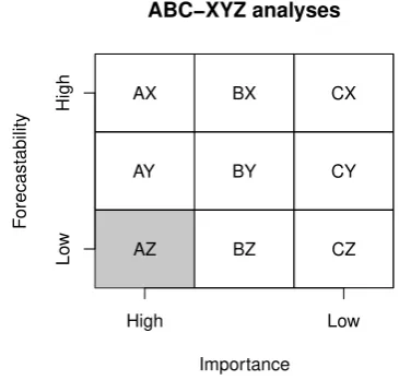
[image:10.595.330.513.527.701.2]

In a standard forecasting and inventory setting, ABC analysis is often used to classify the different stock keeping units (SKUs) into im-portance classes. In this approach, the 20% most important and the 50% least important items are classified as A and C items, respectively. Additionally, XYZ analysis is used in conjunction with ABC analysis to further classify the products into easy-to-forecast (X items) to hard-to-forecast (Z items). As such, nine classes are considered, as depicted in Fig. 7(Ord et al., 2017). We propose the application of the wisdom of crowds for judgmental model selection/build on the AZ items (those of high importance but difficult to forecast). This class is shaded with gray color inFig. 7. In many cases, these items represent only a small frac-tion of the total number of SKUs. Thus, judgmentally weighted selec-tions across the available models of a forecasting support system should be deduced by the individual choices, either in terms of models or patterns, of a small group of managers; our analysis showed that

(11)

selections fromﬁve managers would suﬃce.

A potential limitation of our current study, especially in the big data era, is the number of series and respective contexts examined. As a future direction, we suggest the extension of our study by increasing the amount of time series represented in each context and the number of contexts to allow the evaluation of the robustness of the superior per-formance of the judgmental model selection in each context. This could include more and higher frequencies and exogenous information. Such extensions would also beneﬁt the ongoing limitation of controlled ex-perimental studies towards more generalizable results.

6. Conclusions

Model selection of appropriate forecasting models is an open pro-blem. Optimal ex-ante identification of the best ex-post model can bring significant benefits regarding forecasting performance. The literature has so far focused on automatic/statistical approaches for model se-lection. However, demand managers and forecasting practitioners often tend to ignore system recommendations and apply judgment when se-lecting a forecasting model. This study is thefirst, to the best of our knowledge, to investigate the performance of judgmental model selec-tion.

We devised a behavioral experiment and tested the efficacy of two judgmental approaches to select models, namely simple model selection and model-build. The latter one was based on the judgmental identifi -cation of time series features (trend and seasonality). We compared the performance of these methods against that of a statistical benchmark based on information criteria. Judgmental model-build outperformed both judgmental and statistical model selection. Significant perfor-mance improvements over statistical selection were recorded for the equal-weight combination of statistical and judgmental selection. Judgmental aggregation (weighted combinations of models based on the selections of multiple experts) resulted in the best performance of

any approaches we considered. Finally, an exciting result is that hu-mans are better, compared to statistics, in avoiding the worst model.

The results of this study suggest that companies should consider judgmental forecasting selection as a complementary tool to statistical model selection. Moreover, we believe that applying the judgmental aggregation of a handful of experts to the most important items is a trade-oﬀbetween resources and performance improvement that com-panies should be willing to consider. However, forecasting support systems that incorporate simple graphical interfaces and judgmental identiﬁcation of time series features are a prerequisite to the successful implementation of do-it-yourself (DIY) forecasting. This does not seem too much to ask for software in the big data era.

Given the good performance of judgment in model selection fore-casting tasks, the emulation of human selection processes through ar-tificial intelligence approaches seems a natural way forward toward eventually deriving an alternative statistical approach. We leave this for future research. Furthermore, we expect to further investigate the reasons behind the difference in the performance of judgmental model selection and judgmental model-build. To this end, we plan to run a simplified version of the experiment of this study that will be coupled with the use of an electroencephalogram (EEG) to record electrical brain activity. Future research could also focus on the conditions (in terms of time series characteristics, data availability, and forecasting horizon) under which judgmental model selection brings more benefits. Finally,field experiments would provide further external validity for ourfindings.

Acknowledgments

FP and NK would like to acknowledge the support for conducting this research provided by the Lancaster University Management School Early Career Research Grant MTA7690.

Appendix A. Forecasting models

We denote:

α: smoothing parameter for the level (0≤α≤1). β: smoothing parameter for the trend (0≤β≤1).

γ: smoothing parameter for the seasonal indices (0≤γ≤1). φ: damping parameter (usually)0.8≤ϕ≤1.

y_t: actual (observed) value at period t. lt: smoothed level at the end of period t. bt: smoothed trend at the end of period t. st: smoothed seasonal index at the end of period t.

m: Number of periods within a seasonal cycle (e.g., 4 for quarterly, 12 for monthly).

h: forecast horizon. +

yˆ_{t h}: forecast for h periods ahead from origin t. SES, or ETS(A, N,N), is expressed as:

= + − −

lt αyt (1 α l)t 1, (A.1)

= +

yˆ_{t h} lt. (A.2)

SES with additive seasonality, or ETS(A,N,A), is expressed as:

= − − + − −

lt α y(t st m) (1 α l)t 1, (A.3)

= − + − −

st γ y(t lt) (1 γ s)t m, (A.4)

= +

+ + −

yˆ_{t h} lt st h m. (A.5)

DES, or ETS(A,Ad,N), is expressed as:

= + − − + −

lt αyt (1 α l)(t 1 ϕbt 1), (A.6)

= − − + − −

(12)

∑

= +

+

=

y l h

ϕ b

ˆ_{t h} t .

i i

t

1 (A.8)

DES with additive seasonality, or ETS(A,Ad,A), is expressed as:

= − − + − − + −

lt α y(t st m) (1 α l)(t 1 ϕbt 1), (A.9)

= − − + − −

bt β l(t lt 1) (1 β ϕb) t 1, (A.10)

= − + − −

st γ y(t lt) (1 γ s)t m, (A.11)

∑

= + +

+

=

+ −

y l h

ϕ b s

ˆ_{t h} t .

i i

t t h m

1 (A.12)

[image:12.595.38.559.242.375.2]

Appendix B. Participants details

Table B.6

University modules with at least 20 participants where the behavioral experiment was introduced as an elective exercise.

University Module (and keywords) Level

Bangor University Applied Business Projects: Operations Management (operations, strategy, competitiveness, supply chain, capacity, planning, inventory, forecasting)

PG CardiﬀUniversity Logistics Modelling (business statistics, forecasting, stock control, system dynamics, bull-whip eﬀect,

queuing analysis, simulation)

PG Lancaster University Business Forecasting (time series, forecasting, regression, evaluation, model selection, judgment) UG Lancaster University Forecasting (time series, forecasting, univariate and causal models, evaluation, model selection, judgment) PG National Technical

University of Athens

Forecasting Techniques (time series, forecasting, decomposition, univariate and causal models, evaluation, support systems, judgment)

UG Universidad de Castilla-La

Mancha

Manufacturing planning and control (planning, forecasting, manufacturing, just-in-time, stock control, inventory models)

UG

Table B.7

Industries associated with the practitioner participants.

Industry Participants

Consulting (including analytics) 14

Banking & Finance 11

Software (including forecasting software) 9

Advertising & Marketing 9

Retail 8

Health 8

Government 6

Manufacturing 5

Food & Beverage 4

Energy 3

Logistics 3

Telecommunications 3

Automotive 2

Other 5

References

Abbey, J.D., Meloy, M.G., 2017. Attention by design: using attention checks to detect inattentive respondents and improve data quality. J. Oper. Manag. 53–56, 63–70.

Adya, M., Collopy, F., Armstrong, J.S., Kennedy, M., 2001. Automatic identiﬁcation of time series features for rule-based forecasting. Int. J. Forecast. 17 (2), 143–157.

Alvarado-Valencia, J., Barrero, L.H., Önkal, D., Dennerlein, J.T., 2017. Expertise, cred-ibility of system forecasts and integration methods in judgmental demand fore-casting. Int. J. Forecast. 33 (1), 298–313.

Armstrong, J.S., 2006. Findings from evidence-based forecasting: methods for reducing forecast error. Int. J. Forecast. 22 (3), 583–598.

Armstrong, S.J., 2001. Combining forecasts. In: Principles of Forecasting. International Series in Operations Research & Management Science. Springer, Boston, MA, pp. 417–439.

Ashton, A.H., Ashton, R.H., 1985. Aggregating subjective forecasts: some empirical re-sults. Manag. Sci. 31 (12), 1499–1508.

Athanasopoulos, G., Hyndman, R.J., Kourentzes, N., Petropoulos, F., 2017. Forecasting with temporal hierarchies. Eur. J. Oper. Res. 262 (1), 60–74.

Barrow, D.K., Kourentzes, N., 2016. Distributions of forecasting errors of forecast com-binations: implications for inventory management. Int. J. Prod. Econ. 177, 24–33.

Bates, D., Mächler, M., Bolker, B., Walker, S., 2015. Fitting linear mixed-eﬀects models using lme4. J. Stat. Software 67 (1), 1–48.

Billah, B., King, M.L., Snyder, R., Koehler, A.B., 2006. Exponential smoothing model se-lection for forecasting. Int. J. Forecast. 22 (2), 239–247.

Blattberg, R.C., Hoch, S.J., 1990. Database models and managerial intuition: 50% model + 50% manager. Manag. Sci. 36 (8), 887–899.

Bunn, D., Wright, G., 1991. Interaction of judgemental and statistical forecasting methods: issues & analysis. Manag. Sci. 37 (5), 501–518.

[image:12.595.155.443.424.601.2]