Original citation:
Richings, Gareth and Habershon, Scott. (2017) Direct quantum dynamics using grid-based wavefunction propagation and machine-learned potential energy surfaces. Journal of Chemical Theory and Computation, 13 (9). pp. 4017-4024.
Permanent WRAP URL:
http://wrap.warwick.ac.uk/97112
Copyright and reuse:
The Warwick Research Archive Portal (WRAP) makes this work by researchers of the University of Warwick available open access under the following conditions. Copyright © and all moral rights to the version of the paper presented here belong to the individual author(s) and/or other copyright owners. To the extent reasonable and practicable the material made available in WRAP has been checked for eligibility before being made available.
Copies of full items can be used for personal research or study, educational, or not-for profit purposes without prior permission or charge. Provided that the authors, title and full bibliographic details are credited, a hyperlink and/or URL is given for the original metadata page and the content is not changed in any way.
Publisher’s statement:
This document is the Accepted Manuscript version of a Published Work that appeared in final form in Journal of Chemical Theory and Computation, copyright © American Chemical Society after peer review and technical editing by the publisher.
To access the final edited and published work see
http://dx.doi.org/10.1021/acs.jctc.7b00507
A note on versions:
The version presented here may differ from the published version or, version of record, if you wish to cite this item you are advised to consult the publisher’s version. Please see the ‘permanent WRAP url’ above for details on accessing the published version and note that access may require a subscription.
Direct quantum dynamics using grid-based
wavefunction propagation and machine-learned
potential energy surfaces
Gareth W. Richings and Scott Habershon
∗Department of Chemistry and Centre for Scientific Computing, University of Warwick,
Coventry, CV4 7AL, United Kingdom
E-mail: [email protected]
Abstract
True potential energy
Gaussian process approximation
Ab initio energy evaluations
“On the fly” wavefunction propagation
ѱ(t) ѱ(t+Δt)
1
Introduction
The computer simulation of the dynamical behaviour of molecules is vital in providing
un-derstanding of processes which are important across chemistry, materials science and biology.
Such simulations can be performed using methods based on classical mechanics, but many
processes which are important in biological systems, for example proton transfer mechanisms
in enzyme catalysis1,2 or the photochemistry of DNA3,4 and plant sunscreen molecules,5,6 are
fundamentally quantum mechanical in nature. It follows that simulation methods including
the effects of quantum mechanics are needed to provide an accurate representation of the
system being studied.
To model quantum molecular dynamics we must solve the time-dependent Schr¨odinger
equation (TDSE) for nuclear motion,
i~∂Ψ (q, t)
∂t = ˆHΨ (q, t), (1)
where{q}is the set of degrees-of-freedom (DOFs) of nuclear motion. Methods for following
the time evolution of the wavefunction have been developed and refined over the past few
decades, but among the most successful are those based on expanding the wavefunction in
terms of a grid of basis functions localised in molecular configuration space. The method of
choice in this field is the multi-configuration time-dependent Hartree (MCTDH) approach7–13
which allows the treatment of systems of a few tens of DOFs and converges to the exact
answer given a large enough basis set. Recently, so-called multi-layer MCTDH has been
developed as an extension of the original method, allowing the description of the dynamics
of systems with several hundred DOFs.14–18
The central difficulty of carrying out quantum dynamics calculations using grid-based
methods is the need to define the form of the Hamiltonian operator, ˆH, prior to carrying
out the wavepacket propagation. The nuclear wavefunction evolves on a potential energy
nuclear configuration space. As the wavefunction is a delocalised entity, the global form of
the PES must be known in order to define the Hamiltonian. The fitting of some appropriate
functional form to electronic energies is a common way of determining the PES, for example
using the vibronic coupling Hamiltonian (VCHAM) method,11,12,19,20 but this can be an
arduous process if many nuclear DOFs and/or multiple electronic states are to be included
in the Hamiltonian. The process can be simplified if a convenient choice of coordinate system
is chosen to model the dynamics, but such a choice can often yield a kinetic energy operator
with a complicated form.21
To overcome the problems associated with PES fitting and coodinate system choice,
direct dynamics (DD) methods have been developed recently.22,23 These approaches
circum-vent the long-winded PES fitting procedure by generating the PES during the course of the
dynamics calculation. They avoid the global fitting of the PES by expanding the nuclear
wavefunction in terms of basis functions of particular localised form which mean that only a
localised knowledge of the potential around the centre of the functions is needed. This local
representation also means that the choice of coordinate system is less important as there
is no need to seek a simple global function to represent the PES, meaning that coordinate
systems where the kinetic energy operator has a simple convenient form (e.g. Cartesian
coordinates or normal modes) can be used. Among the most successful DD methods in use
are the trajectory surface hopping (TSH)24–42 and ab initio multiple spawning (AIMS)43–47
methods which have both been used in studies on photochemistry in complex environments.
The former method uses multiple classical trajectories to model the nuclear dynamics, with
ab initio electronic energies being used to provide the forces along the trajectories. AIMS
uses an expansion of the nuclear wavefunction in terms of Gaussian wavepackets, the centres
of which evolve classically while the coefficients of the Gaussians in the wavefunction
ex-pansion are propagated quantum mechanically, with local approximations to the PES used
to evaluate the associated matrix elements. Both methods can model the transfer of the
be-tween the states and AIMS by spawning new Gaussian functions on different states. A fully
quantum mechanical DD method has also been implemented, based on the variational
multi-configuration Gaussian (vMCG) method,48,49 whereby, similar to AIMS, the wavefunction
is represented by a linear combination of Gaussian wavepackets. The vMCG method,
how-ever, employs variational quantum evolution of both the Gaussian basis functions and the
expansion coefficients. The DD-vMCG method50–62 relies on using a Shepard interpolation
of the PES to calculate the matrix elements required for propagation; the electronic energy,
and its gradient and Hessian, are periodically evaluated at the centre of the Gaussian
func-tions, and the local harmonic approximations to the PES that can then be formed around
these points are combined in a weighted sum to give an approximate global PES. Despite
their success, these three popular methods outlined each have issues which makes them less
than ideal when used to model nuclear dynamics; TSH and AIMS rely on classical dynamics
which makes them less able to model such features as tunnelling, while the fully quantum
vMCG method suffers from numerical issues related to the use of a non-orthogonal basis of
Gaussian functions (particularly relating to the linear dependence of the functions causing
singularities in the equations-of-motion50,63).
Ideally a method is required which combines the stability and fully quantum nature of
grid-based dynamics methods, such as MCTDH, with the ease of use and convenience of the
DD methods described above. Although the DD-vMCG method uses an approximation to
the full PES, the Shepard interpolation used is not suitable for MCTDH as it does not have
the required sum-of-products form for efficient propagation of the MCTDH wavefunction.
This desirable aspect of the PES for MCTDH will be considered more fully later but, briefly,
it means that the PES is represented as a linear combination of functions which are products
of separate terms in each DOF.
In this work, we present a new direct grid-based dynamics method based around the use
of Gaussian Process Regression (GPR)64–71 to expand the PES. The roots of this method
rep-resentation of the PES based upon a linear expansion of Gaussian functions distributed
across configuration space, yielding a PES in the sum-of-products form required for efficient
MCTDH simulations. Here, we test this methodology in simulations of two molecules where
intra-molecular proton transfer on the electronic ground state acts as a mechanism for
tau-tomerisation, namely malonaldehyde8–10,17,72–75 and salicylaldimine,50,60,76 both of which are
useful systems for study using quantum dynamics methods due to the role of tunnelling in
the proton dynamics. This work complements a concurrent piece of work carried out by
us, which demonstrated how a similar GPR-based methodology, combined with a
propa-gated diabatisation scheme and a simple two-dimensional wavefunction propagation, could
be used to study excited state dynamics in the butatriene cation;77 this work expands
dra-matically on our previous report by demonstrating that the same GPR approach is suitable
for performing MCTDH simulations, thereby opening up a wide range of future applications.
The remainder of this article is as follows. In the next section we will briefly recap
grid-based dynamics methods, with particular emphasis on MCTDH. We then describe those
aspects of GPR which are relevant to the construction of the PES or quantum dynamics,
followed by details of the implementation of our MCTDH-based DD strategy. In Section 3,
we present the results of dynamics calculations for the proton transfer in malonaldehyde and
salicylaldimine, comparing the results of our new DD method with results obtained using
pre-fitted PESs. We also demonstrate results of dynamics carried out on GPR PESs generated
using ab initio electronic structure data generated “on-the-fly” (i.e. by direct interface to
an electronic structure code during wavefunction propagation). Finally, we conclude by
2
Methodology
2.1
Grid-Based Quantum Dynamics: The Standard Method and
MCTDH
The theory of grid-based methods for solving the nuclear TDSE has been described in detail
elsewhere;7,78 here, we highlight those points most relevant to our proposed grid-based DD
scheme.
Perhaps the most straightforward way to solve the nuclear TDSE is to expand a trial
wavefunction in terms of a time-independent product basis, {χ(jκκ)},
Ψ(q1,· · · , qf, t) = N1
X
j1
· · ·
Nf X
jf
Cj1,···,jf (t)
f
Y
κ=1
χ(jκκ)(qκ)
=X
J
CJ(t)XJ(q)
(2)
where {Cj1,···,jf} is a set of complex, time-dependent coefficients and f is the number of
DOFs in the system; we will discuss the nature of the basis functions later. We have also
introduced the compound index,J=j1,· · · , jf on the second line of Eq. 2 to aid clarity in the
expressions which follow. To model the dynamics we require equations-of-motion (EOMs)
which can be integrated, and to obtain those we use the wavefunction ansatz of Eq. 2 in
Dirac-Frenkel variational principle (DFVP),79,80
hδΨ|Hˆ −i~∂
∂t|Ψi= 0. (3)
After some algebra, we obtain the following EOM to describe the evolution of the
wavefunc-tion coefficients
i~C˙J =
X
L
hXJ|Hˆ|XLiCL. (4)
and with a sufficiently large basis provides a numerically exact solution to the TDSE. We
will refer to this method for solving the TDSE as the standard method hereafter.
The standard method suffer from exponential scaling in computational effort as the
num-ber of DOFs is increased, meaning that for practical purposes f is limited to about 5. To
reduce the effects of this scaling and expand the utility of quantum dynamics methods to
larger molecular systems, the MCTDH method was introduced.7 This method employs the
following ansatz to represent the wavefunction
Ψ(Q1,· · · , Qf, t) = n1 X j1 · · · nm X jm
Aj1,···,jm(t)
m
Y
κ=1
ϕ(jκκ)(Qκ, t)
=X
J
AJ(t) ΦJ(Q, t).
(5)
Here, the wavefunction is defined as a linear combination of Hartree products of
time-dependent basis functions; this is in contrast to the time-independent basis functions of
Eq. 2. The basis functions, which are termed single-particle functions (SPFs), are functions
of single modes of motion, each of which comprises a small number (typically from one
to four) of individual DOFs (i.e. Qκ = (qκ1,· · · , qκp)). Use of a time-dependent basis in
MCTDH ensures that the number of basis functions can be kept small, meaning that the
exponential scaling with system size which afflicts the standard method is minimized.
Individual SPFs are expanded in terms of an underlying, time-independent basis,{Xi(κκ)},
the members of which are functions of the individual modes,
ϕ(jκκ)(Qκ, t) = Nκ X
iκ
c(κ,jκ)
iκ (t)X (κ)
iκ (Qκ). (6)
The basis functions used to represent the SPFs are the same as those used for expanding the
wavefunction in the standard method (Eq. (2)). SPFs describing a mode which consists of
more than one DOF are expanded in terms of products of basis functions along each DOF,
DOF are standard, continuous functions, such as Hermite polynomials or sine functions,
which are transformed into the so-called discrete variable representation (DVR), whereby
the matrix elements of the position operator within the basis are generated and the resulting
matrix diagonalised. The eigenfunctions, localised at evenly spread points in configuration
space (hence forming a ‘grid’), are the DVR basis functions. As these DVR functions are
zero at all gridpoints except the one at which they are centred, the wavepacket is simply
represented by the coefficients of each DVR basis function.
As with the standard method, a set of EOMs is needed to propagate the MCTDH
wave-function, and again the DFVP is used to derive these equations. This time we obtain two
sets of EOMs, one for the wavefunction expansion coefficients, {AJ}, and another for the
SPFs. In their most general form these equations read
i~A˙J =
X
L
hΦJ|Hˆ|ΦLiAL− f X κ=1 nκ X l=1
gj(κ)
κlAJlκ, (7a)
i~ϕ˙(κ) = 1−P(κ)hρ(κ)−1hHˆi(κ)−gˆ(κ)1iϕ(κ)
+ ˆg(κ)1ϕ(κ),
(7b)
where ˆg(κ)is a constraint operator, present due to the redundancy in theansatz, Eq. (5), from
having both time-dependent coefficients and basis functions. In the EOM for the coefficients
we also haveg(jκ)
κl =hϕ
(κ)
jk |gˆ
(κ)|ϕ(κ)
l iandAJlκ =Aj1,···,jκ−1,l,jκ+1,···,jnκ. In the EOM for the SPFs we use the projector onto the space of SPFs in modeκ, ˆP(κ), the inverse of the density matrix
in that mode, ρ(κ)−1, and the mean-field matrix with elements, hHˆi(κ)
jl =hΨ
(κ)
j |Hˆ|Ψ
(κ)
l i. In
this final expression we have used the single-hole functions Ψ(lκ) =P
JκAJκ
lΦJκ, where ΦJκ is the Hartree product of SPFs in all modes apart from mode κ.
Of crucial importance in the work we present here are the matrix elements involving
the Hamiltonian operator in the EOMs above, in particular the potential energy term. To
evaluate the matrix elements of the potential energy operator, ˆV, it is necessary to know the
calculations. The potential matrix elements are integrals over all DOFs (except mode κ in
the case of the mean field operators in Eq. (7b)),
hΦJ|Vˆ|ΦLi=
Z · · ·
Z
Φ∗JV (q1, q2,· · ·, qf) ΦLdq1· · ·dqf. (8)
Evaluating this multidimensional integral is cumbersome and can become a bottleneck in
the dynamics calculation. However, if we can represent the potential in the so-called
sum-of-products form, where individual terms are just sum-of-products of functions of the individual DOFs
(not of the modes, which may contain more than one DOF), such as
V (q1, q2,· · · , qf) =
X i ai f Y κ=1
Vi(qκ) (9)
where the coefficients,{ai}, are independent of the DOFs, then the integral in Eq. (8) reduces
to a sum-of-products of one-dimensional integrals
hΦJ|Vˆ|ΦLi=
X i ai f Y κ=1 Z
ϕ(jκ)∗Vi(qκ)ϕ
(κ)
l dqκ. (10)
Evaluation of the matrix elements in this form is much less arduous than in the
full-dimensional form, hence to fully exploit the efficiency of the MCTDH method it is best
to represent the potential in the form given by Eq. (9). Incidentally, the same arguments
about the form of the operator apply to the kinetic energy operator but, by choice of
ap-propriate DOFs this will naturally be the case and hence the evaluation of kinetic energy
matrix elements is usually straightforward.
The efficiency of evaluation of the PES integrals is increased still further, both for
MCTDH and the standard method, by the use of DVR basis functions. In terms of the
DVR grid-points the potential energy is diagonal such that, for two grid-points centred at
qα and qβ we have
As such we only need to know the value of the PES at the coordinates of the grid-points to
evaluate the PES matrix elements in the DVR basis.
2.2
Gaussian Process Regression
The key development reported here is the implementation of direct grid-based quantum
dynamics using GPR.64–71 This approach, in whichab initio electronic structure calculations
at selected configurations are used to construct a global PES, provides a route to combining
the power of grid-based quantum propagation with local electronic structure calculations;
no prior fitting of the PES is required.
In our strategy, the PES is represented by a linear combination of Gaussian functions,65
centred at a set ofM reference points in configuration space, {qk},
V (q)≈
M
X
k=1
wkexp −α|q−qk|2
. (12)
Here, the parameterα, which determines the width of the Gaussians, defines the length scale
of the fit. If we use standard Cartesian or normal-mode coordinates, we can easily see that
the expansion of the PES matches the sum-of-products form required for efficient MCTDH
wavepacket propagation
V (q)≈
M
X
k=1
wk f
Y
κ=1 exp
−α qκ−qκk
2
. (13)
The weights of the expansion in Eq. (12), {wk}, are determined by solving the set of linear
equations arising from requiring that the M PES values are reproduced at theM reference
configurations, leading to
Kw=b, (14)
where the elements of the vector, b, are the values of the PES at M configurations, qk, for
function. Specifically, we have
bi =V qi
. (15)
The elements of the matrix,K, multiplying the vector of GPR weights, w, are a measure of
the covariance between two members of the set of trial points,65 given here as
Kij = exp −α|qi−qj|2
+γ2δij. (16)
The parameter γ is typically chosen to be a small number and acts to regularise the matrix
so that solution Eq. (14) is numerically well-behaved; more generally, γ can be viewed as
representing the variance (or uncertainty) associated with the PES values in the vector b
(thus, by choosingγ to be some small number in this work, we are implicitly assuming that
the PES values are calculated to a high degree of accuracy, which is most often the case
when using converged electronic structure calculations or an analytical PES).
In practice, GPR is straightforward to implement and, as noted above, is already in a
form which is convenient for MCTDH simulations; however, the key outstanding issue is the
choice of the M reference points used to construct the GPR PES. As noted previously, the
wavefunction propagated in quantum dynamics simulations is non-local in nature, whereas
ab initio electronic structure calculations provide the PES at specific local configurations.
As a result, one approach to selecting the M reference points would be to simply choose
the set of grid-points at which the time-dependent wavefunction would be expected to have
non-zero value during the propagation; however, this approach is no better than the standard
grid-based method and would be expected to suffer from a similar “curse of dimensionality”.
Instead, a better strategy is to select the M GPR reference points in an adaptive manner
during the wavefunction propagation, such that the PES is accurately represented where it is
required for accurate propagation, namely in the vicinity of the time-dependent wavefunction;
this then leads to the question of how one adaptively adds new configurations to the database
GPR PES and the calculated PES at grid-points encountered by the wavefunction during
propagation, and then add the newly-calculated reference point to the database if the GPR
PES is inaccurate beyond some threshold; however, as soon as one is required to calculate
the (possibly computationally-expensive) underlying potential, then this point might as well
be included in the database in any case.
In this work, we address this challenge by using the in-built error measure associated
with GPR. In particular, exploiting the origins of GPR from the field of Bayesian statistics,
it is straightforward to show that the GPR approach outlined above provides a direct way of
assessing the accuracy of the approximate PES without having to calculate the actual PES.
This is achieved using the following variance function which can be evaluated at any point
in configuration space65
σ2(q) = 1 +γ2−kTK−1k. (17)
The parameter, γ, is as defined in Eq. (16) as indeed is the matrix, K. The elements of
the vector, k, are simply the covariances of the point of interest with the current set of M
reference points; in other words, ki = exp (−α|q−qi|2). Thus, Eq. (17) provides a direct
check of whether a new configuration, q, should be added to the GPR reference points;
if σ2(q) is greater than a threshold accuracy value, then the potential, V(q), should be
calculated and added to the GPR reference points. In this way, GPR provides an automated
way of constructing a PES during wavefunction propagation; the implementation of this GPR
PES construction approach in the context of standard and MCTDH quantum dynamics will
now be discussed.
2.3
Implementation
Algorithms for carrying out DD, both for the standard method and MCTDH, with the PES
calculated using GPR have been implemented in a development version of the Quantics
SPFs, initial wavefunction conditions and integration scheme (to integrate Eq. (4) or (7)), are
as previously implemented in the package. We should note, however, that only the variable
mean field integration (VMF) scheme has so far been implemented for solving the MCTDH
EOMs with a GPR PES, with the constant mean field method7 currently being modified.
Our current implementation of grid-based dynamics with “on-the-fly” GPR PESs, can
use either atomic Cartesian coordinate or mass-frequency scaled normal modes as DOFs; this
is currently for computationally simplicity, particularly because the kinetic energy operator
for these coordinate choices are straightforward, but we emphasise that our approach can
in principle be generalized to any appropriate coordinate system. In the case of normal
mode coordinates, it is necessary to provide a transformation matrix between the scaled
normal modes and the Cartesian coordinates, so that the Cartesian coordinates of the atoms
can be passed to a relevant electronic structure program for the evaluation of the potential
energy. The mode transformation matrix can be generated by a standard
normal-mode calculation at a chosen geometry-optimized reference configuration. On running a
calculation, the chosen coordinate set defines the configuration subspace in which the GPR
PES will be constructed; once this subspace has been defined by the user, along with the
other parameters determining the nature of the (standard method or MCTDH) quantum
propagation, the simulation can begin.
To initialise the GPR PES, assuming that we have no prior information about the PES,
we adopt the following procedure. First, the effective width of the wavefunction along the
ith DOF is defined as
hδqii= hΨ|qˆi2|Ψi − hΨ|qˆi|Ψi2
1/2
. (18)
Borrowing from the definition of normal distributions, we equate hδqii with the standard
deviation, σi, of the wavefunction. For a normal distribution, 99.7% of the population is
within 3σi of the mean, therefore we define the limits our sampling space for GPR PES
generation along each DOF ashqii ±3σi,i.e. the subspace within three standard deviations
geometry corresponding to the “centre” of the wavepacket, hqi. Subsequently,N additional
configurations are generated by random uniform sampling for each DOF within the limits
of the sampling subspace defined by the wavepacket centre and standard deviations; in all
calculations reported here, we use N = 100, such that the initial set of reference points in
the GPR PES is M = 101. The potential is then calculated at each reference geometry, for
example using an analytical PES or ab initio electronic structure calculations, hence giving
the vector, b, of potential values at the reference points ( Eq. (15)). TheM reference points
in configuration space are then used to evaluate the matrix K defined in Eq. (16) (using, in
this work, a length parameter α = 0.5) and the linear equations of Eq. (14) are solved to
give the initial vector of GPR weights, w. The solution of the GPR equation is carried out
using Cholesky decomposition routines implemented in LAPACK.82Once the initial weights
have been determined, we then have an initial expression for the GPR PES using Eq. (12).
Following the formation of the initial GPR PES, the wavefunction time-propagation is
allowed to proceed. For each of the M potential terms, there are f individual components
in the Gaussian functions Eq. (13)), one for each DOF in the system. If a mode in the
MCTDH wavefunction, Eq. (5), comprises a single DOF (i.e. the SPFs in that mode are
one-dimensional functions) or a standard method calculation in one-dimension is being
per-formed, then the value of the individual potential term is simply evaluated at each of the
grid-points defined by the DVR basis in which the SPFs or wavefunction are expanded (Eq.
(6)) following Eq. (11). If a multi-dimensional standard method wavefunction or an MCTDH
mode comprising more than one DOF (i.e. the SPFs are multi-dimensional functions) is
be-ing considered then the grid-points in Eq. (2) or Eq. (6) are defined by the correspondbe-ing
number of coordinates. The GPR PES at these grid-points is then evaluated using Eq. (13).
Having completed the procedure of evaluating the potential matrix elements in the DVR
basis, the dynamics proceeds in the usual way; in the MCTDH case, these matrix elements
are transformed to the SPF basis before being used to generate the EOMs (Eq. (7)), which
(4).
The propagation could be allowed to proceed using just the initial set of points to
de-fine the GPR PES but, as the wavepacket evolves, the representation of the PES given by
sampling configuration space with reference to the initial wavepacket is likely to become
increasingly inaccurate; obviously, it is necessary to generate a new representation of the
PES which better reflects the regions of configuration space being sampled during the
dy-namics. It is, of course, possible to generate a new set of random configurations at some
sensible time-interval in the propagation time and to calculateN new PES values, discarding
the previously obtained information about the PES. However, we take a different approach
which is based on the “grow” methodology of Collins and coworkers,83,84 and is similar to
that used in the DD-vMCG method implemented in the Quantics package.
In the approach adopted here, the initial potential values are stored in a database along
with the molecular geometries at which they were calculated (the information is held in
memory during the propagation but also output to file for re-use in subsequent calculations
if needed). The database of configurations and potential energy values is augmented at
regular intervals during the wavepacket propagation by the sampling of configuration space
around the centre of the wavepacket in the same way as the initial sampling. At each of
the sampled configurations, the GPR variance as defined in Eq. (17) is calculated (using the
database points from previous evaluations only, so as to avoid repeated matrix inversions).
If the variance is below some threshold (in this work taken to be 10−6), then it is considered
that the current GPR PES representation at that configurations is sufficiently accurate, such
that no new potential energy values need to be calculated. However, if the variance is greater
than the threshold, then a new energy is calculated and stored in the database. Once any
new points have been added to the database, Eq. (14) is solved once again (including all
energies in the database) to give a new set of GPR weights and hence a new form for the
PES. The wavepacket propagation then proceeds, adding new database points and updating
propagation with “on the fly” evaluation of the PES; furthermore, as noted above, the
GPR PES constructed using the potential energy evaluations is already in a form which is
convenient for MCTDH propagation.
Naturally, the PES available during the early stages of the propagation is likely to be
less accurate than that constructed later in time, when more database points are used to
generate the GPR PES; as a result, once an initial calculation is complete, it is possible
to re-run the dynamics using the full database from the start. This second propagation
can be run without adding any new points to the database or with the option of adding
new database points according to the threshold conditions outlined above. In principle the
propagation could be repeated in the latter manner until no more points are added and
the GPR PES can be considered converged (at least for the regions of configuration space
sampled during the total propagation time with the same initial wavepacket conditions).
In the simulations reported below, single calculations have been performed to generate the
PES before subsequent wavepacket propagations using the database created during the prior
calculation.
Finally, to calculate potential energy values at sampled configurations during
wavefunc-tion propagawavefunc-tion, our implementawavefunc-tion uses much of the machinery in Quantics put in place
to perform DD-vMCG calculations by interfacing with assortedab initio electronic structure
programs. In practice the program creates an input file at the geometry of interest, calls the
external quantum chemistry package, then reads the appropriate information (in the case
considered here, just the total electronic energy) from the resulting output file. Furthermore,
we note that we can also perform GPR PES-based simulations of any PES, not just those
generated by electronic structure calculations; this fact is used later to benchmark our new
3
Results
To demonstrate the abilities of our direct grid-based dynamics methods, the ground-state
dynamics of the intramolecular proton transfer for two different molecules has been
stud-ied. Such processes are characterised by the double-well nature of the PESs on which they
occur, arising from two local minima corresponding to the hydrogen bonded to different
atoms, separated by a potential barrier. Double well potentials are ideally suited to testing
new quantum dynamics methods because they often feature strongly quantum-mechanical
tunnelling processes which are difficult, if not impossible, to accurately reproducevia other
non-quantum methods.
[image:19.612.228.400.309.451.2](a) (b)
Figure 1: Two molecules of interest in this work: (a) Malonaldehyde and (b) Salicylaldimine. In both case the dynamics of the transfer of the proton bonded to an oxygen atom in these pictures is considered; in the former case to the other oxygen and in the latter to the nitrogen.
3.1
Malonaldehyde
As the first test of our grid-based DD method, we consider the ground electronic state
dynamics of the intramolecular proton transfer in malonaldehyde (Fig. 1(a)). The aim of
this study is to test the ability of dynamics performed on a GPR approximation to the PES
to replicate those observed on a known PES. In this way, we can directly assess whether
surfaces generated using our GPR method are accurate representations of the underlying
Recently, an accurate PES for the ground state of malonaldehyde was reported by
Mizukamiet al, fitted to energies calculated at the HF/QZVPP level with
fc-CCSD(T)(F12*)/def2-TZVPP correlation energies.72 We have integrated the subroutine published by them into
the Quantics package so as to be able to generate potential energies at molecular geometry
sampled by the dynamics, and hence be able to run dynamics using either the fitted PES or
the direct dynamics approach using a GPR PES.
Two calculations were performed on a 3-dimensional subsystem of malonaldehyde, both
using the standard method (Eq. (2)), the first just using the full Mizukami PES (evaluated
on all grid-points) and the second using a GPR representation of the PES generated
“on-the-fly” using the implementation described in Section 2.3. The dynamics was performed
in dimensionless, mass-frequency scaled normal mode coordinates, where the normal mode
transformation matrix was calculated by diagonalising the mass-weighted Hessian matrix
determined at the proton transfer transition state geometry given previously.72
The three normal modes chosen to carry out the dynamics were the proton transfer mode
(v1 of frequency 1321.32icm−1), the out-of-plane motion of the proton (v12 of frequency
1290.31 cm−1) and the in-plane OHO bending mode (v18 of frequency 1899.62 cm−1). For
both calculations a sine DVR basis with 101 grid-points was used for v1 and a harmonic
oscillator DVR basis was used for the other modes, with 21 functions each. The initial
wavepacket was constructed as a Gaussian function of width 0.7 along all modes, centred at
v1=0.5 andv11=v18=0.0. The dynamics was run using the short iterative Lanczos propagator
of order 15, and was followed for 100 fs. In the case of the direct dynamics calculation, the
PES was sampled, as described in Section 2.3, every 1 fs.
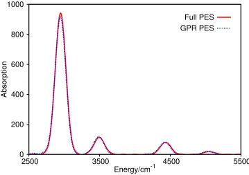
First, we compare the vibrational spectrum of the 3-dimensional malonaldehyde model
calculated using the full grid-based standard method and our GPR-based DD method. This
spectrum was calculated by Fourier transforming the autocorrelation function, defined as
The value ofG(t) was output every 1 fs during the course of both calculations. The procedure
for performing this transform is described in detail elsewhere, particularly concerning the use
of a damping function to ensure that the function reaches zero at the end of the propagation
in order to avoid artefacts in the spectrum.7
In Fig. 2, we present the vibrational spectra of 3-mode malonaldehyde resulting from these
two calculations. Clearly, the two spectra are in excellent agreement, with each showing four
main peaks. The most intense peak in both cases is centred at 2949 cm−1, the intensity
of the peak differing by less than 3% between the two calculations. The next two peaks in
increasing energy order do not quite coincide between the calculations, the GPR peaks being
centred 6 cm−1 lower in energy than those from the full calculation in both cases, but again
have very similar intensities. The highest energy peak around 5040 cm−1 differ in position
by 13 cm−1 between the calculations and by 12% in intensity.
0 200 400 600 800 1000
2500 3500 4500 5500
Absorption
Energy/cm-1
[image:21.612.126.485.364.617.2]Full PES GPR PES
Overall, the differences between the spectra are very small, indicating that the GPR
representation of the PES is very accurate. The discrepancies, in the energies and intensities
of the peaks, between the two calculations are simply due to the small variation in the shape
of the PES, leading to small shifts in the vibrational energy levels. This is particularly so
early on in the wavepacket propagation, where fewer energy points have been calculated and
hence the number of terms in Eq. (12) is less.
We have implied that the representation of the GPR PES at later stages in the
propaga-tion should be more accurate than that at earlier times due to the addipropaga-tion of extra reference
configurations to the GPR expansion; this point is clearly demonstrated in the next
compar-ison. During the initial DD calculation, 2425 points in configuration space were sampled; as
noted in Section 2.3, the calculated potential energies are saved on file and can be re-used
in subsequent calculations. To this end, a second propagation was run, using a GPR PES
calculated at the start of the propagation using all 2425 reference energies; no further points
were added during this second propagation. The resulting spectrum is visually identical in
shape to that resulting from the full calculation, all peaks aligning with one another exactly.
The intensities of the lowest energy peak differ between the two calculations by only 0.015%
whilst those of the highest energy peak differ by less than 3%. This result indicates that,
given an adequate sampling of configuration space, GPR can reproduce the shape of the
underlying PES almost exactly.
A more sensitive test of the dynamics than the vibrational spectrum is the measurement
of the wavepacket flux through a dividing surface. The flux can be measured as the rate
of change of wavefunction population in the region beyond the dividing surface.7 Using a
step function defined along some DOF,θ(q−qγ), whereqγ is the coordinate of the dividing
surface, the population to the positive side of the surface is hΨ|θ(q−qγ)|Ψi. Applying
Ehrenfest’s theorem,78 the rate of change of the population is7
d
dthΨ|θ(q−qγ)|Ψi= i
The flux operator is thus defined as ˆF=i
~[ ˆH,θ(q−qγ)].
The flux expectation value was evaluated every 1 fs during the three wavepacket
propa-gations described above, with the dividing surface placed perpendicular to the v1 mode at
the location of the transition state between the two equivalent isomers (i.e. v1=0). Figure
3 shows the calculated flux expectation values for the three calculations: standard method
dynamics on the full PES, single-run GPR-based DD propagation, and GPR-based DD
propagation using previously-sampled energies. Comparing these results, it is clear that DD
accurately reproduces the quantum dynamics of the system as the wavefunction propagates.
In all three cases, there is an initial movement of the wavepacket from the right-hand side
of the barrier (positive v1 coordinate) towards the left-hand potential well, followed by a
periodic crossing and re-crossing with period of just over 40 fs. This process involves
tunnel-ing through the barrier, demonstrattunnel-ing that our DD method can cope with this feature of
dynamics; in other words, the GPR PES describes the two potential wells and the potential
barrier with sufficient accuracy to reproduce the correct wavefunction tunnelling.
As with the vibrational spectrum, there is very good agreement between the results of
the full dynamics and those of the initial DD run. Not only is the overall form of the
time-dependent flux reproduced, but small features such as the spikes in flux during the first 10 fs
are also reproduced. The flux calculated using DD on the final database gives even better
agreement with the results from the full dynamics. The agreement is not perfect, with some
small discrepancies creeping in particularly at later times (for example the small plateaus in
the flux at about 45 fs and 50 fs are not seen in either DD calculation, and some of the fine
structure towards the end of the propagation is missing). However, the ability of the DD
method to reproduce the wavepacket flux accurately is a further indication that the GPR
-0.2 -0.1 0.0 0.1 0.2
0 20 40 60 80 100
Flux
Time/fs
Full PES
GPR PES: Created
[image:24.612.129.483.75.323.2]GPR PES: Read
Figure 3: Plot of the flux operator expectation value, G(t), for a three mode model of malonaldehyde. The dividing surface is placed at the barrier of the transition mode, v1. All potential energies were calculated from the surface of Mizukami et al.72 The solid, red line is the result of the calculation performed using the full dynamics. The hashed, blue line is the result of the calculation with the potential constructed using the GPR process, sampling points in configuration space as explained in the text. The dashed, green line is the result of the calculation with the potential constructed using GPR process on a pre-calculated database of potential energies.
3.2
Salicylaldimine
As a second test system, we look at the proton transfer process in salicylaldimine (Fig. 1(b)).
Here, the proton moves between the oxygen atom (the imine or enol form) and the nitrogen
atom (the amine or keto form), the former being the more stable structure of the two. In
contrast to malonaldehyde, there are thus two distinct tautomers to consider, and the PES
is not symmetric about the barrier separating the energy minima which correspond to each
tautomer.
An analytical PES, fitted using the VCHAM approach for 13 of the normal modes of
salicylaldimine (calculated at the transition state geometry between the optimised keto and
compare the standard, grid-based dynamics and DD results. Contrary to the original report,
the 3-21G basis set was used along with the restricted Hartree-Fock method to generate
energies to which the PES was fitted. In this work we will use the previously-fitted PES
to generate benchmark results against which to compare our DD scheme. We consider two
cases here: (i) a two-dimensional version, which is sufficiently small that the standard (grid)
method of propagation can be used (thereby minimizing errors arising due to wavefunction
propagation itself, allowing us to focus on the accuracy with which GPR can reproduce the
underlying PES), and (ii) a six-dimensional version, where we use MCTDH, combined with
GPR, to perform quantum dynamics “on the fly”. Furthermore, we will also compare these
results to GPR PESs calculated by direct interface with an external ab initio electronic
structure code, in this case ORCA,85 marking the first time that MCTDH simulations have
been performed “on the fly”.
3.2.1 2D Dynamics
The first comparison we make uses a two-dimensional model of salicylaldimine, the normal
modes chosen being those termed v1 and v36 by Polyak et al; these are the proton transfer
mode and in-plane OHN bending mode, respectively. As only two DOFs were involved in
the calculation, it was possible to run standard method dynamics for (i) the full fitted PES,
(ii) a GPR PES representation generated in DD simulations of the fitted Polyak surface, and
(iii) a GPR PES representation generated using DD simulations and electronic structure
energies calculated “on-the-fly”. All calculations used a sine DVR basis with 121 functions
along thev1 mode and a harmonic oscillator DVR basis comprising 21 grid-points alongv36.
The initial wavepacket was constructed as a 2D Gaussian function centred at v1=0.96 and
v36=0.14 with widths hdv1i=0.5706 and hdv36i=0.7704. This starting configuration places
the system to the enol side of the barrier between the two tautomers (the transition structure
is at the origin of the coordinate system). Propagations were performed for 100 fs with data
-0.15 -0.10 -0.05 0.00 0.05 0.10
0 20 40 60 80 100
Flux
Time/fs
Fitted PES
GPR PES: Fitted
[image:26.612.130.481.75.324.2]GPR PES: ORCA
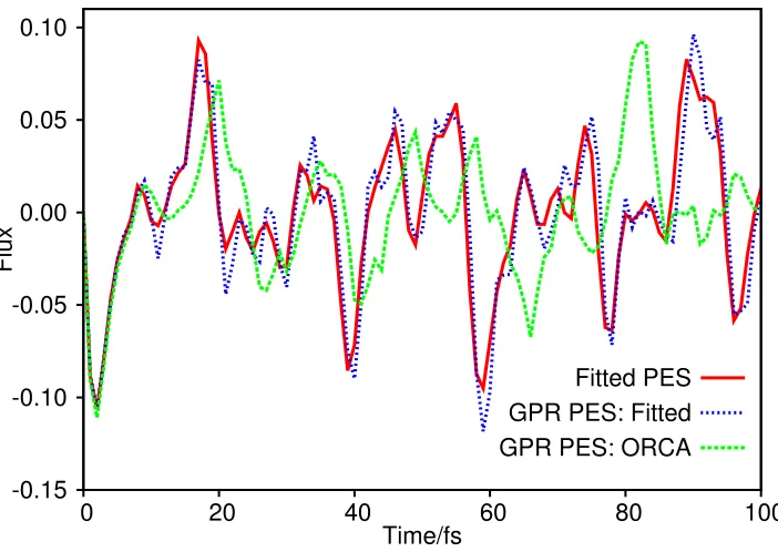
Figure 4: Plot of the flux operator expectation value for a two degree-of-freedom model of salicylaldimine. The dividing surface is placed at the barrier of the transition mode, v1. The solid, red line is the result of using the full dynamics. The hashed, blue line is the result of the calculation with the potential constructed using the GPR process, sampling points in configuration space as explained in the text. In both cases the potential energies were calculated from the surface of Polyak et al.60 The dashed, green line is the result of the calculation with the potential constructed using the GPR process, with energies calculated by calls to ORCA, “on-the-fly”.
Figure 4 shows the wavefunction flux through a surface perpendicular to the proton
transfer mode, placed at the peak of the transition barrier between the tautomers (v1=0),
allowing us to follow the tautomerization process over the course of the propagation time;
results are shown for all three calculations. We first compare the flux of the wavefunction
moving on the fitted surface to the wavefunction flux on the PES approximated using GPR
sampling on the fitted PES. Clearly the two curves are very similar to one another; the
initial, negative flux indicating proton transfer across the potential barrier towards the keto
tautomer, followed by a re-crossing of the barrier to the enol side. Later in the dynamics
there are short periods of crossing one way or the other, each lasting only a few femtoseconds.
very closely for the entire duration of the dynamics. The correspondence is particularly
good early in the dynamics, degrading slightly at later times, with the flux on the GPR
PES lagging behind that on the full, fitted PES. In the DD GPR simulation, 353 potential
energies were calculated during the course of the propagation; as expected, restarting the
simulation using this full GPR reference set (not shown) gives even better agreement with
that calculated using the full fitted surface. The results from the initial comparison reinforce
the conclusion drawn from the calculations on malonaldehyde, namely that a GPR PES can
give a very good representation of the underlying PES. As an aside, we note that our GPR
PES scheme required far fewer PES evaluations than the total number of grid-points in this
two-dimensional case (21×121 = 2541).
The second comparison we can make when examining Fig. 4 is between the fluxes
cal-culated using the fitted PES and the flux determined from dynamics performed on a GPR
PES calculated using ab initio energies evaluated “on-the-fly”. In constructing theab initio
GPR PES, the sampling of configuration space around the wavepacket centre is performed
in the same way as described in Section 2.3; however, the potentials are calculated using
RHF/3-21G so as to match the level of theory used by Polyaket al in performing their
DD-vMCG calculations. From Fig. 4, during the first 10 fs or so, the flux follows that calculated
using the fitted potential (i.e. the initial crossing to the keto side of the barrier); however,
after this point the flux diverges from that calculated using the fitted surfaces. This plot
can be best compared to Fig. 4(d) in the Polyak paper,60 where a DD-vMCG calculation
was performed for this system; specifically, the difference between the ab initio and fitted
PES observed in our DD simulations are similar to the differences observed between the
DD-vMCG result using “on-the-fly” PES evaluation and vMCG using the fitted PES. In
this previous work, the discrepancy between the two results is attributed to the form of the
potential on the enol side of the barrier which made the fitting of the potential along thev36
difficult for the VCHAM method. The flux calculated using a potential constructed by an
performing DD-vMCG calculations, should thus be a more accurate reflection of the true
dynamics. This result, and the comparison to previous DD-vMCG results, clearly shows
that it is possible to perform direct grid-based dynamics calculations using a PES generated
“on-the-fly” using ab initio data.
3.2.2 6D Dynamics
The second set of calculations performed on salicylaldimine uses six normal modes; two of
these are the same as in the 2D case above (ν1 and ν36), with the four additional modes
la-belledν10,ν11,ν13andν32in the work by Polyaket al (see Fig. 2 in reference 60 for diagrams
of the motions, all of which are in-plane modes). We note that these six modes are the same
as those considered in previous DD-vMCG simulations. We perform the same comparison
as performed in the previous section; specifically, we compare (i) dynamics on the fitted
PES, (ii) dynamics on a GPR approximation to the fitted surface, and (iii) direct-dynamics
with a GPR approximation to the PES generated by “on-the-fly” electronic structure
calcu-lations. In the 6D case, however, there are too many DOFs to use the standard grid-based
wavefunction propagation method, so we use MCTDH for all three calculations.
Following previous simulations of salicylaldimine, our calculations all used a wavefunction
ansatz constructed in terms of three sets of 2D SPFs, with the DOFs being grouped as
{ν1, ν36}, {ν10, ν11} and {ν13, ν32}. The propagations were run for 100 fs using the
Adams-Bashforth-Moulton predictor-corrector integrator of sixth order to solve the EOMs using an
accuracy parameter of 10−5 (these settings are the default for the VMF integration scheme
in Quantics). The MCTDH calculation on the fitted PES used 18 SPFs in each mode, and
the calculations using the GPR approximation to the PES (both to the fitted PES and to
the ab initio points) required 30 SPFs per mode. This increase in the number of SPFs was
necessary due to the highly correlated nature of the form of the potential when using GPR
(i.e. all DOFs are coupled, being involved as they are in all potential terms, whereas the
the SPFs was a set of 101 sine DVR functions along ν1 and 21 harmonic oscillator DVR
functions along the other five modes. The initial wavepacket was centred at hν1i=0.96,
hν36i=0.14, and hν10i=hν11i=hν13i=hν32i=0.0, with widths of hδν1i=0.5706, hδν10i=0.7745,
hδν11i=0.7590, hδν13i=0.6902,hδν32i=0.6707 and hδν36i=0.7704.
In Fig. 5 we present two plots showing results from these calculations; both show plots
of the wavepacket flux through a dividing surface perpendicular to the stretching mode,ν1,
and at the peak of the transition barrier (as in the 2D case). Looking first at Fig. 5(a) we
show the results of: (i) the MCTDH calculation on the fitted PES (the full result), (ii) the
initial MCTDH calculation using a GPR approximation to the fitted PES (with electronic
energies being added every 1 fs), and (iii) an MCTDH calculation performed using the GPR
approximation to the fitted PES, using the database created by the previous calculation.
In Fig. 5(b) we repeat the plot of the full result for clarity along with a plot of the flux
generated by an MCTDH calculation using a GPR PES generated by calculating
RHF/3-21G electronic energies with ORCA “on-the-fly” (the database is updated every 1 fs). Again,
Fig. 5(b) also shows the flux for a subsequent calculation employing MCTDH using a GPR
PES constructed using the database of energies created in the previous calculation.
Making an initial comparison of the plots in Fig. 5 with those in Fig. 4, we see that,
after an initial move towards the keto isomer (indicated by the negative flux), there is far
less overall movement of the wavepacket across the potential barrier in the 6D case than
in the 2D case across the 100 fs period of simulated dynamics. The reason for this is that
the presence of more DOFs, each of which is coupled to the others, allows the wavepacket
to spread and move in directions which do not take it over the barrier; in the 2D case the
wavepacket is constrained to move in only two directions, one of which is across the barrier
where the flux is being measured, so more structure is seen in Fig. 4 than in Fig. 5.
Looking now at each figure in turn, we begin with Fig. 5(a) where the dynamics in all
three calculations was based on the fitted PES of Polyak et al.60 The solid, red line is the
-0.15 -0.10 -0.05 0.00 0.05
Flux
Fitted PES
GPR PES: Fitted Initial
GPR PES: Fitted Read
(a)
-0.15 -0.10 -0.05 0.00 0.05
0 20 40 60 80 100
Flux
Time/fs
Fitted PES
GPR PES: ORCA Initial
[image:30.612.136.494.81.550.2]GPR PES: ORCA Read (b)
be compared. The full MCTDH result indicates an initial, rapid flow of the wavepacket
over the barrier towards the keto tautomer, followed by an oscillation back towards the enol
form; all of this occurs within the first 10 fs of the dynamics. There is a subsequent, small
move in the same direction followed by motion in the positive flux direction towards the
enol tautomer around 20 fs. This motion slows to close to zero until there is more motion
in the enol direction between 40 and 50 fs, followed by a 20 fs period of movement in the
keto direction (the trough centred on 60 fs). The most significant move towards the enol
side of the potential barrier of the whole dynamics occurs around 80 fs. The final 10 fs of the
dynamics is characterised by a lack of motion across the barrier.
Examining the results of the initial calculation using a GPR potential (hashed, blue line
in Fig. 5(a)), where potential energy values from the fitted PES were added every 1 fs during
the dynamics, we see that the initial motion of the wavepacket across the barrier to the keto
tautomer is qualitatively correct, if somewhat overestimated. The plot rejoins that of the
full result around the 10 fs point, and there is a subsequent, small motion towards the keto
tautomer, again, as seen in the full result but likewise overestimated. As with the full result,
the flux then heads in the positive direction, but unlike the full result, it quickly falls back
to zero. From this point on, the two plots do not closely correspond; the flux of the GPR
calculation turns negative between 30 and 60 fs before going positive until 80 fs, then back
to zero and finally into the positive region to the end of the calculation. Clearly the initial
potential generated “on-the-fly” is not accurate enough to closely reproduce the flux of the
full result but, at the same time, not so inaccurate as to get the dynamics completely wrong.
To further assess the accuracy of the GPR PES, the dynamics was repeated using a
GPR PES calculated using the energies generated during the initial propagation; the results
of this are shown by the dashed, green line in Fig. 5(a). It is immediately apparent that
the dynamics much more closely matches the full result than the initial calculation. The
first 10 fs of the plot almost exactly matches the that of the full result, whilst the period of
qualitatively matches that of the full result, in particular the period of negative flux between
50 and 70 fs and that of positive flux for the 20 fs afterwards correspond to the full result
quite well. The match is not perfect, but it is clear that the underlying dynamics is well
represented; in other words, the GPR procedure gives a good approximation to the potential
from which it is derived.
In spite of this success, these MCTDH results highlight one downside of our method,
namely the growth in the number of Gaussians needed to represent the PES. Recall from
Section 3.2.1 that 353 Gaussians were needed to accurately represent a 2D PES, whilst in
section 3.1, 2425 Gaussians were needed for a 3D PES (admittedly for a different molecule).
In this 6D calculation, 10101 database points were generated, the maximum possible in this
particular calculation (an initial point at the wavefunction centre, then 100 points at each
femtosecond, 0 to 100). Clearly the number of Gaussians needed to accurately represent the
PES increases rapidly as the dimensionality of the problem rises. This is less of an issue
when using the standard method for the dynamics as it is only necessary to know the actual
value of the potential at the location of each DVR point, not the contributions from each
Gaussian in the GPR; the PES in that case is completely determined by a single number for
each gridpoint, which can be evaluated and saved whenever the energy database is updated.
On the other hand, the structure of the MCTDH EOMs means that it is the value of each
term in the GPR expansion of the potential along the DOFs making up each set of SPFs that
is required; in other words the potential has to be dealt with term by term. In the case of
6D salicylaldimine, there are thus 10101 terms in the potential which have to be calculated
and then combined in the Hamiltonian and mean-field integrals in Eq. (7). This number
of terms in the potential operator means that calculations become very time-consuming as
more DOFs are added; we come back to this point later.
Moving on to consider Fig. 5(b), we note the same issues with computational effort,
as just outlined, when propagations are performed using a GPR PES generated using ab
calculated, each of which naturally required a call to the ORCA program. As with Fig.
5(a) the solid, red line is the result of the flux for the MCTDH calculation on a fitted PES,
repeated for clarity in comparison with the new results performed on an ab initio GPR
PES. The first new result to examine is that represented by the hashed, blue line, which is
generated by performing dynamics on a GPR PES built from ab initio energies added to an
initially empty database. As with the calculations using the fitted surface (Fig. 5(a)), we
see an overestimated negative flux during the first 10 fs, which does not quite return to zero
at 10 fs, but slows down there, only reaching zero after about 25 fs. From this point onwards
the flux is fairly featureless, staying close to zero, except for a short period of negative flux
between 40 and 50 fs. The plot is not particularly smooth (as in the corresponding plot in
Fig. 5(a)) because the updates to the potential at every femtosecond cause the global PES
to shift slightly, hence affecting the motion of the wavepacket.
The dashed, green line represents the results of the subsequent calculation using a GPR
PES based on the 10101ab initio energies calculated during the previous propagation. Here
the initial period of negative flux matches that of the MCTDH calculation on the fitted
surfaces, both in intensity and duration. The flux is then positive until 25 fs and then
returns to zero until about 50 fs. The flux then has a bump upwards into positive territory
until about 60 fs, before a period in the negative direction for the next 20 fs, then a final
up and down to the end of the propagation. Clearly the dynamics does not match that
of the full (MCTDH, fitted surface) result, but it should not be expected to because the
GPR PES in this case is an interpolation of the actual HF/3-21G PES, rather than of a
fitted approximation to it. The close agreement in the first few femtoseconds occurs when
the wavepacket is localised relatively close to the origin of the coordinate system, the point
around which the VCHAM fitted potential is expanded. The fit will be most accurate around
this region,i.e.most closely resembling the interpolation of the GPR, hence the similarity in
the dynamics. The differences in the potential are more pronounced further from this point,
are best compared to Fig. 6 in Ref. 60, where a DD-vMCG calculation on the same system
was performed. Making this comparison, we see that the plots of the flux match really quite
well with the DD-vMCG results, with the major features reproduced. This indicates that
the approach outlined here, using electronic energies calculated “on-the-fly”, gives dynamics
which closely agree with those from a well established alternative DD method.
As a final note, it is worth commenting on the computational effort of these simulations.
The 6D MCTDH simulation coupled to HF/3-21G calculations took approximately 186h
walltime on the first run and then 639h for the run using the pre-calculated database; both
were parallelised across 16 processors. The 6D MCTDH calculation on the original fitted
PES required 69h walltime for the run generating the database of points with the second
calculation taking 143h (again both were parallelised over 16 processors). However, the
important point of our approach is that the PES is generated “on the fly”; there is no need
for laborious pre-fitting of the PES, and the associated challenges surrounding appropriate
choice of coordinates, functional forms, and so on. As a result, and bearing in mind that the
approach highlighted in this Article is far from optimized with regards to both methodology
and code implementation, we expect that our DD MCTDH scheme to quickly evolve into
a useful and highly-accurate computational tool for studying quantum dynamics in both
ground-state and excited-state systems.
4
Conclusions
We have presented initial results for a new direct quantum dynamics scheme which combines
well-established grid-based dynamics methods (standard method and MCTDH) with PESs
created using GPR with electronic energies calculated “on-the-fly” either from a pre-fitted
potential or from an electronic structure package. To the best of our knowledge, this is the
first implementation of a DD version of MCTDH.
have shown that the GPR representation of the PES is capable of almost exactly matching the
underlying potential by comparison to results from pre-fitted PESs. This followed through
to calculations on a 6D model of salicylaldimine using MCTDH, but the computational
effort required means that convergence of the potential in terms of the number of Gaussians
becomes a major difficulty, leading to inaccuracies in the dynamics.
The computational effort required is even greater when calculating electronic energies
“on-the-fly” using an electronic structure package. However, the results from these
cal-culations are very promising, with good agreement to the DD-vMCG results of Polyak et
al. We have thus shown that it is possible to perform MCTDH-based quantum dynamics
calculations without the need to pre-compute the PES.
Future work will focus on reducing the computational resources needed to perform
MCTDH/GPR calculations on systems with more than a few degrees-of-freedom. Potential
ideas to be investigated include the use of an additive kernel for the GPR, where, instead
of using a sum of f-dimensional Gaussians as in Eq. (12), each term is a sum of lower
di-mensional Gaussian functions,70 potentially leading to efficiencies in evaluating PES matrix
elements. It is also possible to include PES gradient information in GPR, and this may offer
another route to minimising computational effort, however, it remains to. be seen whether
the increased effort in calculating energy gradients counteracts any gains made. Another
possible development which we are exploring is to take the GPR representation and use
it as a basis for generating a more compact representation of the PES in the style of the
well-known high-dimensional model representation (HDMR) strategy.86,87
As noted in the Introduction, we have already implemented the method outlined here
for multiple electronic states, so it is clear that, if improved efficiency can be achieved,
the proposed method has the potential to be of great utility to those wishing to carry out
Acknowledgements
We are grateful to the Leverhulme Trust for funding (RPG-2016-055), and to the Scientific
Computing Research Technology Platform at the University of Warwick for providing
compu-tational resources. The data from Figs. 2-5 can be found at http://wrap.warwick.ac.uk/id/eprint/88404.
References
(1) Boekelheide, N.; Salom´on-Ferrer, R.; Miller III, T. F. Dynamics and dissipation in
enzyme catalysis. Proc. Nat. Acad. Sci. USA 2011, 108, 16159–16163.
(2) Masgrau, L.; Roujeinikova, A.; Johannissen, L. O.; Hothi, P.; Basran, J.;
Ranaghan, K. E.; Mulholland, A. J.; Sutcliffe, M. J.; Scrutton, N. S.; Leys, D. Atomic
Description of an Enzyme Reaction Dominated by Proton Tunneling. Science 2006,
312, 237–241.
(3) Middleton, C. T.; de La Harpe, K.; Su, C.; Law, Y. K.; Crespo-Hern´andez, C. E.;
Kohler, B. DNA excited-state dynamics: from single bases to the double helix. Annu.
Rev. Phys. Chem. 2009, 60, 217–239.
(4) Stavros, V. G.; Verlet, J. R. Gas-Phase Femtosecond Particle Spectroscopy: A
Bottom-Up Approach to Nucleotide Dynamics.Annual Review of Physical Chemistry 2016,67,
211–232.
(5) Baker, L. A.; Horbury, M. D.; Greenough, S. E.; Allais, F.; Walsh, P. S.; Habershon, S.;
Stavros, V. G. Ultrafast Photoprotecting Sunscreens in Natural Plants.J. Phys. Chem.
Letters 2016, 7, 56–61.
(6) Baker, L. A.; Greenough, S. E.; Stavros, V. G. A Perspective on the Ultrafast
Photo-chemistry of Solution-Phase Sunscreen Molecules. The Journal of Physical Chemistry
(7) Beck, M. H.; J¨ackle, A.; Worth, G. A.; Meyer, H. D. The multiconfiguration
time-dependent Hartree (MCTDH) method: A highly efficient algorithm for propagating
wavepackets. Phys. Rep.2000,324, 1–105.
(8) Schr¨oder, M.; Gatti, F.; Meyer, H.-D. Theoretical studies of the tunneling splitting
of malonaldehyde using the multiconfiguration time-dependent Hartree approach. J.
Chem. Phys.2011,134, 234307/1–9.
(9) Schr¨oder, M.; Meyer, H.-D. Calculation of the vibrational excited states of
malonalde-hyde and their tunneling splittings with the multi-configuration time-dependent Hartree
method. J. Chem. Phys. 2014, 141, 034116/1–13.
(10) Coutino-Neto, M.; Viel, A.; Manthe, U. The ground state tunneling splitting of
mal-onaldehyde: Accurate full dimensionl quantum dynamics calculations. J. Chem. Phys.
2004, 121, 9207–9210.
(11) Neville, S.; Worth, G. A reinterpretation of the electronic spectrum of pyrrole: A
quantum dynamics study. J. Chem. Phys. 2014,140, 034317/1–13.
(12) Giri, K.; Chapman, E.; Sanz, C. S.; Worth, G. A full-dimensional coupled-surface
study of the photodissociation dynamics of ammonia using the multiconfiguration
time-dependent Hartree method .J. Chem. Phys. 2011, 135, 044311/1–13.
(13) Sadri, K.; Lauvergnat, D.; Gatti, F.; Meyer, H.-D. Rovibrational spectroscopy using
a kinetic energy operator in Eckart frame and the multi-configuration time-dependent
Hartree (MCTDH) approach. J. Chem. Phys. 2014, 141, 114101/1–11.
(14) Wang, H.; Thoss, M. Multilayer formulation of the multiconfiguration time-dependent
Hartree theory.J. Chem. Phys. 2003, 119, 1289–1299.
(15) Wang, H. Multilayer Multiconfiguration Time-Dependent Hartree Theory. J. Phys.
(16) Vendrell, O.; Meyer, H.-D. Multilayer multiconfiguration time-dependent Hartree
method: Implementation and applications to a Henon-Heiles Hamiltonian and to
pyrazine. J. Chem. Phys. 2011,134, 044135/1–16.
(17) Hammer, T.; Manthe, U. Intramolecular proton trnasfer in malonaldehyde: Accurate
multilayer multi-configurational time-dependent Hartree calculations. J. Chem. Phys.
2011, 134, 224305/1–11.
(18) Manthe, U. The multi-configuration time-dependent Hartree approach revisited. J.
Chem. Phys.2015,142, 244109/1–15.
(19) K¨oppel, H.; Domcke, W.; Cederbaum, L. S. Multimode molecular Dynamics beyond
the Born-Oppenheimer approximation. Adv. Chem. Phys. 1984, 57, 59–246.
(20) Cederbaum, L. S.; K¨oppel, H.; Domcke, W. Multimode vibronic coupling effects in
molecules. Int. J. Quant. Chem. 1981,15, 251–267.
(21) Meyer, H.-D., Gatti, F., Worth, G. A., Eds. Multidimensional quantum dynamics:
MCTDH theory and applications; Wiley: Weinheim, Germany, 2009.
(22) Persico, M.; Granucci, G. An overview of nonadiabatic dynamics simulation methods,
with focus on the direct approach versus the fitting of potential energy surfaces. Theo.
Chem. Acc. 2014,133, 1526/1–28.
(23) Worth, G. A.; Robb, M. A.; Lasorne, B. Solving the time-dependent Schr¨odinger
Equa-tion in one step: Direct Dynamics of Non-adiabatic Systems. Mol. Phys. 2008, 106,
2077–2091.
(24) Tully, J. C.; Preston, R. K. Trajectory surface hopping approach to nonadiabatic
molec-ular collisions: The reaction of H+ with D
2. J. Chem. Phys. 1971, 55, 562–572.
(25) Tully, J. C. Molecular dynamics with electronic transitions. J. Chem. Phys. 1990, 93,