Please cite this paper as:
Svetunkov Ivan and Boylan John E. (2017). Multiplicative State-Space Models for Intermittent Time Series. Working Paper of Department of Management Science, Lancaster University, 2017:4 , 1–43.
Managmeent Science
Working Paper 2017:4
Multiplicative State-Space Models
for Intermittent Time Series
Ivan Svetunkov and John E. Boylan
The Department of Management Science
Lancaster University Management School
Lancaster LA1 4YX
UK
© Ivan Svetunkov
All rights reserved. Short sections of text, not to exceed two paragraphs, may be quoted without explicit permission,
provided that full acknowledgment is given.
Multiplicative State-Space Models
for Intermittent Time Series
Ivan Svetunkova,∗, John E. Boylana
aCentre for Marketing Analytics and Forecasting
Lancaster University Management School, Lancaster, LA1 4YX, UK
Abstract
Intermittent demand forecasting is an important supply chain task, which is commonly done using methods based on exponential smoothing. These methods however do not have underlying statistical models, which limits their generalisation. In this paper we propose a general state-space model that takes intermittence of data into account, extending the taxonomy of exponential smoothing models. We show that this model has a connection with conventional non-intermittent state space models and underlies Cros-ton’s and Teunter-Syntetos-Babai (TSB) forecasting methods. We discuss properties of the proposed models and show how a selection can be made between them in the proposed framework. We then conduct experiments on simulated data and on two real life datasets, demonstrating advantages of the proposed approach.
Keywords: Inventory forecasting, state space models, exponential smoothing, intermittent demand, Croston, count data
1. Introduction
An intermittent time series is a series that has non-zero values occurring at irregular frequency. The data is usually, but not necessarily, discrete and often takes low integer values. Intermittent series occur in many application areas where there are rare events. Examples include security breaches, nat-ural disasters and the occurrence of demand for slow-moving products. In
∗Correspondence: Ivan Svetunkov, Department of Management Science, Lancaster
Uni-versity Management School, Lancaster, Lancashire, LA1 4YX, UK.
the last case we usually refer to “intermittent demand” which, in addition to irregularity of occurrence, contains only zeroes and positive values. The final application area is important in a supply-chain setting, where decisions need to be made about the quantity to order and the discontinuation of ordering. In this paper, we establish a general modelling framework for intermittent series, which does not depend on any particular application area. However, its development has been motivated by the requirements of inventory man-agement. Two forecasting methods that have been described in the supply-chain literature to inform how much to order and when to discontinue a product, are Croston’s method (Croston, 1972) and the TSB method (Te-unter et al., 2011). Neither of these methods has, so far, been furnished with a satisfactory statistical model.
From a practical supply-chain perspective, there are a number of issues that need to be resolved. We need to decide, in a systematic way, which intermittent demand forecasting method to use, rather than allowing these choices to be arbitrary. Having chosen the forecasting method, it needs to be parametrised appropriately. Finally, replenishment decisions should be informed by reliable estimates. For inventory systems based on the probabil-ity of stock-out, good estimates of upper percentiles of demand are required. For systems based on fill-rates (percentage of demand filled immediately from stock), good estimates of probabilities of demand are required. In the latter case, these may be calculated from an estimated Cumulative Distribution Function. The modelling approach recommended in this paper supports the estimation of both percentiles and Cumulative Distribution Functions. In-deed, we argue that a sound statistical model can support method choice, parametrisation and, ultimately, replenishment decisions in supply chains.
2. Literature review
The most popular intermittent demand forecasting method was proposed by Croston (1972). His method has been researched extensively in recent years and has been implemented in widely adopted supply chain software packages (e.g. SAP APO). Croston was the first to note that, when demand is intermittent, simple exponential smoothing produces biased forecasts im-mediately after demand occurrences (known as ‘decision-point bias’). So he proposed splitting the observed data into two parts: demand sizes and de-mand occurrences. The proposed model in Croston (1972) has the following simple form:
yt =otzt, (1) where ot is a binary Bernoulli distributed variable taking a value of one when demand occurs and zero otherwise andzt is demand size, having some conditional distribution. Proposing the model (1), Croston suggested to work with each of these two parts separately, showing that the probability of occurrence can be estimated using intervals between demands. If qt is the time elapsed since the last non-zero observation, then it represents the demand interval when the next non-zero observation occurs. Both demand sizes zt and demand intervals qt are forecasted in this method using simple exponential smoothing, which leads to the following system:
ˆ
yt= qˆ1tzˆt ˆ
zt=αzzt−1+ (1−αz)ˆzt−1 ˆ
qt =αqqt−1+ (1−αq)ˆqt−1
, (2)
where ˆyt is the predicted mean demand, ˆzt is the predicted demand size and ˆ
qt is the predicted demand interval andαq and αz are smoothing parameters for intervals and sizes respectively. In Croston’s initial formulation it was assumed that αq = αz, but separate smoothing parameters were later sug-gested by Schultz (1987), and this additional flexibility has been supported by other researchers (e.g. Snyder, 2002; Kourentzes, 2014). Note that the update of variables ˆqt and ˆzt happens in the method (2) only when ot = 1. When ot= 0, then there is no updating, ˆzt= ˆzt−1 and ˆqt = ˆqt−1.
Syntetos-Boylan Approximation, SBA):
ˆ
yt=
1− αq 2
1
ˆ
qt ˆ
zt. (3)
They conducted an experiment on 3000 real time series and showed that forecasting accuracy of SBA is higher than Croston’s method (Syntetos and Boylan, 2005).
Although various models have been proposed, none have so far been iden-tified which would be appropriate for non-negative integer series and would underlie Croston’s method. This means that heuristic methods of initialisa-tion and parameter estimainitialisa-tion are used instead of statistically rigorous ones. Several authors over the years have looked into this problem.
Snyder (2002) discussed possible statistical models underlying Croston’s method. He examined the following form:
yt=otµt|t−1+t, (4) where µt|t−1 is the conditional expectation of demand sizes. Snyder (2002) showed that the model (4) contradicts some basic assumptions about inter-mittent demand. The main reason for this is because the error term t is assumed to be normally distributed, but this means that demand can be negative. So, Snyder (2002) proposed the following modified intermittent demand model:
yt+ =otexp(µt|t−1+t), (5) where yt+ represents the demand at timet.
Shenstone and Hyndman (2005) studied several possible statistical models with additive errors, including those of Snyder (2002), to identify a model for which Croston’s method is optimal. They argued that any model underlying Croston’s method must be non-stationary and defined on continuous space including negative values. They concluded that such a model has unrealistic properties.
(Hyndman et al., 2008, pp. 281 - 283) proposed a model underlying Croston’s method based on a Poisson distribution of demand sizes with time varying parameter λt:
yt=otzt
zt∼Poisson(λt−1−1) + 1
λt=αzzt−1+ (1−αz)λt−1
ot∼Bernoulli
1 qt
qt =αpτt−1+ (1−αp)qt−1
, (6)
where λt is the average number of events per trial and τt is the observed demand intervals. The authors point out that the proposed model “gives one-step-ahead forecasts equivalent to Croston’s method”. This is because the conditional expectation ofztfor one-step-ahead in (6) is equal toλt−1−1+1 =
λt−1, which corresponds to Croston’s ˆzt in (2). However, the proposed model has two problems.
First, (6) cannot be considered as an appropriate statistical model, be-cause it uses the SES method for λt, without giving a rationale for the gen-erating process. The system of equations (6) should be considered as a filter instead. It still retains useful statistical properties, but it is not as powerful as appropriate statistical models, and sidesteps the ETS taxonomy. Fur-thermore although the Poisson distribution becomes closer to the normal distribution with an increase ofλ, the connection between the model (6) and the conventional ETS models is not apparent, making two separate cases. The authors also do not propose any statistical model underlying the de-mand intervals qt and once again use SES. This limits the properties of the occurrence part of the model to the specific forecasting method.
Second, using the filter described in (6) restricts its generalisation, be-cause introduction of new components or exogenous variables is not straight-forward in this framework.
Overall, while the filter (6) solves some problems for intermittent demand, and has a connection with Croston’s method, it cannot be considered as a complete solution to the problem.
as the Poisson one, discussed above. In addition, although it is well-known that with the increase of trials the Binomial distribution asymptotically be-comes equivalent to the normal distribution, it cannot be explicitly used when the probability of success is equal to one, because it is not supported in this case. Furthermore because the authors did not model the occurrence variable separately, the proposed Negative Binomial filter is more restrictive than the filter (6). Finally, the authors did not make a comparison with the ETS(A,N,N) model in their paper, so it is not possible to assess the accuracy advantage of the proposed filters in comparison with the simpler non-intermittent models.
Another intermittent demand method was proposed by Teunter et al. (2011), which has been known in the literature as TSB. It was derived for obsolescence of inventory, but can be used for other cases as well. The authors proposed using the same principle as in (1), but estimating the time vary-ing probability of demand occurrence pt using simple exponential smoothing based on the variableotrather than switching to intervals between demands. Their method can be represented by the following system of equations:
ˆ
yt= ˆptˆzt ˆ
zt=αzzt−1 + (1−αz)ˆzt−1 ˆ
pt =αpot−1+ (1−αp)ˆpt−1.
, (7)
where ˆpt is the predicted probability of demand occurrence and αp is the smoothing parameter for this probability estimate. The update of probabil-ity in TSB is done after each observation, while demand sizes are updated only when ot = 1. In cases when ot = 0 there is no updating, ˆzt = ˆzt−1. An advantage of this method is that the conditional expectation does not need any corrections similar to (3). However the authors did not propose a statistical model for their method, which leads to issues similar to the ones for Croston’s method. These include problems with the correct estimation of the model parameters, conditional mean and variance.
3. Statistical model
3.1. Filter or statistical model?
Before proceeding to the main part of the paper, it is important to discuss two forecasting approaches, that are often met in the literature, namely using filters and using statistical models.
The filtering approach assumes that the data is used as an input of some equation (or set of equations) and is transformed into a value of the same scale as the original data. The classical example of a filter is Simple Exponential Smoothing (SES), which has the form:
ˆ
yt=αyt−1+ (1−α)ˆyt−1, (8) where α is the smoothing constant. The advantage of filters is in their sim-plicity and the small number of assumptions. For example, SES is very easy to interpret and can be used without assuming normality of the residuals. The main disadvantage of filters is in the lack of statistical rationale. This leads to ambiguity in estimation of the parameters of the filter and problems in the construction of prediction intervals. For example, different initialisa-tion procedures and different estimators can be applied to (8) and there is no way to say which of them should be preferred without a rigorous analysis of its predictive performance. This was one of the main arguments against us-ing exponential smoothus-ing in the statistical literature and one of the reasons that statisticians used to prefer ARIMA models to exponential smoothing (Box and Jenkins, 1976). Finally, the selection of a filter appropriate to the data is one of the problems that does not have a straightforward solution. Both Croston’s and TSB methods are filters.
Overall, both approaches are used in practice and both of them have advantages and disadvantages. In this paper we employ the modelling ap-proach, keeping in mind its upsides and downsides mentioned above.
3.2. General Intermittent State-Space Model
We start from Croston’s original formulation (1) and split intermittent demand into two parts in a similar way, but assuming that zt is generated using a statistical model on its own. We argue that the assumption that the error term interacts with the final demand yt rather than demand sizes zt is the main flaw in the logic of derivation of statistical models underlying intermittent demand forecasting methods. Moving the error term into zt allows using any statistical model that a researcher prefers (e.g. ARIMA, ETS, regression, diffusion model etc). The model underlying zt corresponds to potential demand for a product, while the other model, underlying ot, corresponds to demand realisations, when a customer makes a purchase of a product.
Taking into account that both Croston’s method and TSB use exponential smoothing methods, we propose to use a model form that underlies this forecasting approach. We adopt the single source of error (SSOE) state-space model, as this has been well-established (Snyder, 1985; Hyndman et al., 2002) whilst acknowledging that other model forms are possible (e.g. multiple source of error, MSOE). We use the SSOE model for zt, which in a very general way has the following form, based on (1):
yt=otzt
zt =w(vt−1) +r(vt−1)t vt=f(vt−1) +g(vt−1)t
, (9)
where ot is a Bernoulli distributed random variable, vt is the state vector,
In our new model, the first equation corresponds to Croston’s original formulation (1), while the second equation, called the measurement equation, reflects the potential demand size evolution over time. The third equation is the standard transition equation for an SSOE model, describing the change of components of the model over time.
An interpretation of the new intermittent demand model (9) is that a potential demand size may change in time even when an actual demand is not observed. In these cases, ot = 0, leading to yt = 0 in the first equation of (9). However the measurement and the transition equations in (9) are not affected byot, leading to potential evolution ofztregardless of whether there is an actual demand occurrence or not.
One thing to note about this model is that it can be applied to inter-mittent data with continuous non-zero observations. Such series arise in the context of natural disasters and other natural phenomena. They are less common in a supply chain context, but time series with such characteristics do exist. For example, daily sales of an expensive coffee sold per ounce can exhibit such behaviour with zeroes in some days and then fractional quanti-ties in the others.
However, while the model (9) solves the problem identified by Shenstone and Hyndman (2005) of negative values (because now a multiplicative model can be used for zt), there is still a need for an integer-valued model. In order to solve this problem, we propose a simple modification of the first equation in (9):
yt =otdzte, (10) where dzte is the rounded up value of zt. This way the statistical model we propose becomes integer-valued, and it does not contradict any reasonable assumptions about intermittent demand. Furthermore, any statistical model can be used for zt. It is worth noting that the rounding is an important issue, which will be explored further in this paper, in Section 3.7. But before looking into model (10) we need to study the properties of the basic model (9), keeping in mind that it is an approximation of the more realistic model (10).
The model with rounded up values will be called in this paper “integer” model, while the simpler model (9) will be referred to as “continuous”.
In order for the model (9) to work we make the following assumptions, some of which can be relaxed and would lead to different models:
discussed later in this paper, in Section 3.7.
2. Demand size zt is independent of its occurrence ot. Relaxing this as-sumption will lead to a different statistical model;
3. Potential demand size may change in time even if we do not observe it. Relaxing this assumption means that we need to impose additional restrictions on the transition equation;
4. othas a Bernoulli distribution with some probabilityptthat in the most general case varies in time. This is a natural assumption, following the idea of Croston (1972). Making some other assumption in its place will also lead to a different statistical model.
With these assumptions the proposed intermittent state-space model al-lows calculating conditional expectation and variance for several steps ahead using the following formulae:
µy,t+h|t=µo,t+h|tµz,t+h|t
σ2
y,t+h|t=σo,t2 +h|tσz,t2 +h|t+σo,t2 +h|tµ2z,t+h|t+µo,t2 +h|tσz,t2 +h|t
, (11)
where µy,t+h|t and σ2y,t+h|t are respectively conditional expectation and con-ditional variance of yt; µo,t+h|t and σo,t2 +h|t are conditional expectation and variance of occurrence variable ot and finally µz,t+h|t and σz,t2 +h|t are the re-spective values for the demand sizes zt.
The important point is that, taking into account intermittent demand, pure multiplicative models make more sense for the measurement equation in (9) than additive or mixed ones, because they restrict the space of de-mand sizes to positive numbers. In this paper we discuss the multiplicative error ETS model for demand sizes, namely ETS(M,N,N), which denotes mul-tiplicative error, no trend and no seasonality. The reason for this choice is because ETS(M,N,N) is a simple well-known model underlying simple expo-nential smoothing (Hyndman et al., 2008, p.54), which is a core method in both Croston and TSB. However more complicated models can also be used instead of ETS(M,N,N), but they are not of the main interest in this paper. The general continuous intermittent state-space model (9) reduces to the special case, called iETS(M,N,N), and can be written as:
yt=otlz,t−1(1 +t)
lz,t=lz,t−1(1 +αzt), (12) wherelz,tis the level of the series of non-zero observations andlz,t−1(1 +t) =
with location parameters µ and σ2: (1 +t) ∼ logN(µ, σ2). The general properties of the ETS(M,N,N) model with the proposed assumptions are discussed briefly in Appendix A.
The statistical model (12) is useful because it allows estimating all the pa-rameters via likelihood maximisation. The concentrated log-likelihood func-tion for the model (12) in case of log-normal distribufunc-tion of error has the following form (see Appendix B for the derivation):
`(θ,σˆ2|Y) = −
T1
2 log(2πe) + log( ˆσ
2)−X ot=1
log(zt)
+X
ot=1
log(ˆpt) +X ot=0
log(1−pˆt) , (13)
whereθ is the vector of parameters to estimate (initial values and smoothing parameters),T1is the number of non-zero observations, ˆσ2 = T11 Pot=1log
2
(1 +t) is the variance of the one-step-ahead forecast error for the demand sizes and
ˆ
pt is the estimated probability of a non-zero demand at time t. This like-lihood function allows estimation of the parameters of iETS models and implementation of model selection even between different intermittent and conventional ETS models.
The only variable that still needs to be estimated is the probability pt, which can be modelled in different ways. In the simplest case it can be assumed that it is fixed, meaning that:
ot∼Bernoulli(p). (14)
In more complicated cases it may vary in time, leading to a Croston’s style approach:
ot∼Bernoulli
1 1 +qt
(15) or an approach in the TSB style:
ot∼Bernoulli(pt). (16)
as iETSI (acknowledging that the occurrence part is modelled via demand intervals) and the model with the case (16) as iETSP (pointing out that the probability is modelled directly). We drop the part denoting the type of ETS model used for demand sizes, implying that the ETS(M,N,N) is the standard model for demand sizes.
In this paper we discuss four types of models: with fixed, Croston’s, TSB probability and the one selected automatically between the three. The model without any specified probability does not have a subscript.
3.3. iETSF – the model with fixed probability
This is the simplest model. It is formulated in the following system of equations:
yt=otlz,t−1(1 +t)
lz,t =lz,t−1(1 +αzt)
ot∼Bernoulli(p) (1 +t)∼logN(µ, σ2)
. (17)
In this model we assume that the probability of demand occurrence is fixed. The conditional expectation of the occurrence variable ot can be then calcu-lated as:
µo,t+h|t=p. (18) The conditional variance of demand occurrence does not change over time as well and is equal to:
σo,t2 +h|t =p(1−p). (19) Finally the conditional expectation and variance for intermittent demand can be calculated using (see derivations in Appendix C):
µy,t+h|t=pµz,t+h|t
σ2
y,t+h|t =pσz,t2 +h|t+p(1−p)µ2z,t+h|t
. (20)
In order to estimate this model we use the log-likelihood function (13), which with the assumption of fixed probability becomes simpler. The probability
p can then be estimated via the maximisation of the likelihood:
ˆ
p= T1
T , (21)
(which is needed for information criteria) is equal to four: initial value lz,0, smoothing parameter αz, variance σ2
and the probability p. The location parameter µ is usually assumed to be equal to zero, so that the underlying normal distribution has zero mean. However if the parameter is not equal to zero, then it should be taken into account, increasing the number of param-eters by one.
3.4. iETSI – the model with Croston’s probability
It is assumed in Croston’s method that the probability of occurrence pt does not change between demand sizes that we observe, and that the intervals
qtbetween demands are inversely proportional to the probability. Taking this into account, the occurence part of iETSI in Croston style can be formulated as:
ot ∼Bernoulli
1 1+qt
qt=lq,t−1(1 +q,t)
lq,t =lq,t−1(1 +αqq,t) (1 +q,t)∼logN(µq, σq2)
, (22)
where lq,t is the level component for intervals between demands, αq is the smoothing parameter andq,tis the error term of demand intervals. The error term implies that the demand intervals have their own stochastic nature, so even if the level of intervals is fixed, the actual observed intervals may have their own variability. Note that the interval variable qt is continuous in the model (22), distributed log-normally and defined on (0,∞). But in many applications it is often the case that we can only observe integer-valued intervals ˜qt. So we deal with discretisation of a continuous unobservable variable due to the process of measurement of data. This imposes some restrictions on the model (22), because the observed ˜qt will have a discrete log-normal distribution and will be represented by integer numbers greater than zero with the smallest value of ˜qt = 1 in contrast with (1 +qt) always being greater than one. So the observed intervals ˜qt can be set equal todqte. This means that the first equation in (22) should be amended in order to make the model more realistic:
ot ∼Bernoulli
1 dqte
, (23)
finally the model that underlies Croston’s method and can be estimated on data collected in discrete time has the following form:
yt=otlz,t−1(1 +t)
lz,t=lz,t−1(1 +αzt) (1 +t)∼logN(µ, σ2)
ot ∼Bernoulli
1
dqte
qt=lq,t−1(1 +q,t)
lq,t =lq,t−1(1 +αqq,t) (1 +q,t)∼logN(µq, σq2)
. (24)
It is also important to note that although the intervals qt may vary in time on each observation, influencing the corresponding probabilitypt, iETSI model cannot be estimated when demand is zero. So during the estimation of the model it is assumed that the states of qtdo not change between demand occurrences. This may be an artificial assumption but it follows logically from the original Croston’s method.
Finally it follows straight from the connection between simple exponen-tial smoothing and ETS(M,N,N) that Croston’s method (2) has (24) as an underlying statistical model. Note that this implies that the method has an underlying intermittent model with continuous demand sizes.
Overall, the usage of continuous distribution for demand intervals in the model is motivated by the following:
1. We assume that the demand intervals are continuous in their nature, and only their measurement makes them integer;
2. Using the continuous ETS(M,N,N) model for demand intervals shows the connection of the iETSI model with Croston’s method;
3. The model for demand intervals becomes extendable. This means that in future research it is easy to modify the demand intervals part of the model, introducing different time series components and exogenous variables.
Taking into account the discussion of sample paths of ETS(M,N,N) in Appendix A based on (A.1), it can be noted that iETSI model implies one of the two cases:
1. If expµq+ σ2
q 2
of occurrence will converge to one. So in this case the demand changes from slow moving to fast moving.
2. If expµq+ σ2
q 2
>1, thenqtwill diverge, meaning that the probability of occurrence becomes close to zero, which characterises the obsoles-cence of a product.
Although the latter is implied by the model, it cannot be correctly estimated because of the aforementioned updating properties of Croston’s method. This means that iETSI model should be more efficient for the former cases.
We can also calculate conditional (on the information available on the observation t) expectation and variance of the model, which depend on value of qt. The former is straightforward and is equal to:
µo,t+h|t=E pt+h|t
=E
1
qt+h|t
. (25)
Syntetos and Boylan (2001, 2005) showed that the conditional expectation in Croston’s method is biased and proposed a correction, but we do not incorporate it here for reasons discussed later in Section 3.6. Knowing the value (25) and using the Bernoulli distribution assumption, the conditional variance of the occurrence part can be calculated as:
σo,t2 +h|t=µo,t+h|t(1−µo,t+h|t). (26)
Because the model underlying the occurrence part of Croston’s method is ETS(M,N,N), its parameters can be estimated by maximising the likelihood function of the log-normal distribution. In order to estimate the likelihood of the final intermittent demand model (13), we would need to derive the density function forpt. However it can be shown (see Appendix D) that for the estimation of the occurrence part of the model (24), a likelihood, derived from the assumption of log-normal distributions of (1 +q,t), can be used directly:
`(θ,σˆ2|Y) =−
Tq
2 log(2πe) + log( ˆσ 2 q)
−X
ot=1
log(qt), (27)
where ˆσ2 q = T1q
PTq
(25) for each observation t can be inserted in (13) instead of ˆpt in order to obtain the following concentrated likelihood:
`(θ,σˆ2|Y) =−T1
2 log(2πe) + log(ˆσ 2)
−X
ot=1
log(zt)
+X
ot=1
log (ˆpt) +X ot=0
log (1−pˆt) . (28)
This simplifies the estimation process of the iETSI model as it can now be done in two steps:
1. Estimation of parameters of the demand occurrence part of the model using (27);
2. Estimation of parameters of the demand size part of the model using (28).
In order to calculate information criteria we need to know the number of parameters used in the model. While the demand sizes part of the model is still the same, the occurrence part now has a smoothing parameter and its own variance along with the initial value. So the number of parameters in (24) is equal to six: initial value lz,0, smoothing parameter αz, variance ˆσ2, initial value lq,0, the smoothing parameter αq and the variance ˆσ2q.
Note that any multiplicative ETS model could potentially be used instead of ETS(M,N,N) in the demand occurrence part of (24), including models with exogenous variables. This enlarges the spectrum of potential intermittent demand models. However we do not aim to study all these models in this paper.
3.5. iETSP – the model with TSB probability
Similarly to Croston’s method, it is assumed in TSB that the probability of demand occurrence may vary in time, which means that it has its own conditional expectation and variance. In order to model this behaviour we use a Beta distribution for the probability of occurrence. This means that we need to deal with a compound Beta-Bernoulli distribution:
well in intermittent demand forecasting (Dolgui and Pashkevich, 2008a,b). However, in previous papers it was assumed that the parameters of the Beta distribution do not vary in time, while our modification assumes that both parameters of the Beta distribution may change in time. In order to model this we propose using two ETS(M,N,N) models, which leads to the following large state-space model:
yt=otlz,t−1(1 +t)
lz,t=lz,t−1(1 +αzt) (1 +t)∼logN(µ, σ2)
ot∼Beta-Bernoulli (at, bt)
at=la,t−1(1 +a,t)
la,t=la,t−1(1 +αaa,t) (1 +a,t)∼logN(µa, σa2)
bt=lb,t−1(1 +b,t)
lb,t=lb,t−1(1 +αbb,t) (1 +b,t)∼logN(µb, σb2)
, (30)
where la,t and lb,t are levels for each of the shape parameters,a,t and b,t are mutually independent error terms and αa and αb are the smoothing param-eters. Similarly to previous models, error terms are distributed log-normally with location parametersµa,µb,σa2 andσb2. This guarantees that both shape parameters are positive.
Using the properties of sample paths discussed in Appendix A, we can show that (30) allows modelling the following four situations:
1. If expµa+σ
2
a 2
≤ 1 and expµb+σ
2
b 2
≤ 1, then the sample paths of both at and bt will converge to zero (either asymptotically or al-most surely), in which case the Beta distribution becomes equivalent to Bernoulli withp= 0.5.
2. If both expµa+ σ
2
a 2
> 1 and expµb+σ
2
b 2
> 1, then at and bt will diverge, meaning that distribution of probabilitypt is concentrated around 0.5. This means once again that asymptotically p= 0.5. 3. If expµa+ σ
2
a 2
≤ 1 while expµb+ σ2
b 2
4. If expµa+ σ
2
a 2
>1 while expµb+ σ2
b 2
≤1, then the sample path of
atwill diverge, while the sample path ofbtwill converge to zero. In this case the Beta distribution becomes degenerate with values concentrated around one, which means that a product switches from slow moving to fast moving.
So, in general, model (30) underlies a wide variety of real life processes. How-ever, the TSB method is underpinned by a more specific model, because it does not have the part corresponding to bt. In order to derive the connec-tion between the model (30) and the TSB method we need to impose the following restriction:
at+bt= 1, at∈(0,1) (31) This means that instead of using two models for shape parameters we can use only one:
at=la,t−1(1 +a,t)
la,t =la,t−1(1 +αaa,t). (32) In turn, this means that the expectation of the Beta-distributed probability
pt can be simplified to:
E(pt) = E
at
at+bt
= E(at) =la,t−1. (33)
The very same expectation is calculated in the TSB method (7), which im-plies that the model (32) underlies the occurrence part of the TSB method, because ETS(M,N,N) underlies the simple exponential smoothing method. However there is one important element – this connection implies thatat =ot and bt = 1−ot – which is not realistic, because the density function of the Beta distribution is equal to zero for cases of at = 0 or bt = 0. This means that the model (30) will underlie TSB only when the difference between at and ot is infinitesimal. In order to estimate this model, we can introduce the following approximation for at:
at=ot(1−2κ) +κ, (34) where κ is a very small number (for example,κ= 10−10). This modification is artificial but it helps estimation of the model. It is worth stressing that κ
So, summarising all of the derivations above, the following model under-lies TSB:
yt=otlz,t−1(1 +t)
lz,t=lz,t−1(1 +αt) (1 +t)∼logN(µ, σ2)
ot∼Beta-Bernoulli (at,1−at)
at=la,t−1(1 +a,t)
la,t=la,t−1(1 +αaa,t) (1 +a,t)∼logN(µa, σ2a)
, (35)
where (34) is used purely for model estimation purposes. The model (35) will have only two sample paths cases out of four, corresponding to items (3) and (4) in the list above. So this model is suitable for modelling demand for products that either become obsolete or fast moving. However there is a potential problem with the model (35) in the case (4), becauseatcan become greater than one, implying that bt = 1−at<0. In this situation the model does not make sense. So iETSP model (35) implies that there is only one sensible situation, corresponding to item (3) of the list: when at decreases and converges almost surely or asymptotically to zero, while bt converges to one.
Once again we may use a likelihood function for estimation of the model (35). It can be derived using the same likelihood as in (13) (see Appendix E for the details):
`(θ,σˆ2|Y) = −
T1
2 log(2πe) + log( ˆσ 2)
−X
ot=1
log(zt)
+X
ot=1
log(la,t−1) +
X
ot=0
log(1−la,t−1)
. (36)
Taking into account that demand sizes are independent of demand occur-rences in the proposed model, the latter can be optimised separately by minimising the following cost function (instead of maximising the compound Beta-Bernoulli likelihood directly):
CF =−X ot=1
log (la,t−1)−
X
ot=0
log (1−la,t−1). (37)
The conditional mean and variance of the demand occurrence part of the iETSP model are much simpler to calculate than in iETSI model. They are:
µo,t+h|t=la,t
σ2
o,t+h|t =la,t(1−la,t). (38) Finally, due to (37), there is no need to estimate the variance of the occurrence part of the model (35). This means that the iETSP model has only five parameters: initial valuelz,0, smoothing parameterαz, variance ˆσ2, initial value la,0 and the smoothing parameter αa.
Once again any other multiplicative ETS model can be used instead of ETS(M,N,N) in (35), which leads to completely new types of models. But this is yet another potential research direction.
3.6. Conditional values and prediction intervals for iETS models
One of the advantages of statistical models, as discussed in section 3.1 is the ability to work with distributions of variables rather than point values. For intermittent state-space models, there are some peculiarities that need to be taken into account, which are mainly caused by the assumption of log-normal distribution of residuals.
It has already been discussed that the mean of the log-normal distribution can be calculated based on location parameters µ and σ2 using (A.1):
E(1 +t) = exp
µ+
σ2 2
.
However in cases of skewed distributions, the median value is usually consid-ered to be more robust and useful than the mean. It can be shown that the conditional median of zt+h|t can be calculated using (see Appendix F):
Md(zt+h|t) =lz,t. (39)
mean, it can be calculated using (A.1). However this means that the mod-els will produce different point forecasts than Croston’s method and TSB. Furthermore, if (A.1) is used for the final calculation, the forecast trajectory may demonstrate increase over time, because the variance in (A.1) typically increases with the increase of the forecast horizon. That is why this will not be discussed further in this paper.
The formula (39) also implies that Croston’s method in our formulation does not need any bias correction, because Md x1= Md(1x).
All of the above also means that the final forecasts produced by all the models discussed in this paper are not mean forecasts, but a multiplication of median forecasts for demand sizes and the median of demand occurrence parts. Although this is not what is usually used in forecasting, we argue that this is not a critical issue, because for the typical task of inventory management it is more important to have a distribution of values rather than a single value.
In order to calculate prediction intervals for intermittent state-space mod-els, the cumulative distribution function (CDF) can be used:
F(yt+h < x) = µo,t+h|tFh(zt+h < x) + (1−µo,t+h|t), (40) where Fh(zt+h) is the h-steps ahead CDF for zt+h and x is the value of the desired quantile of the distribution. In order to find the appropriate x for intervals of a desired width, an optimisation procedure can be used for each horizonh. In this procedure the parameters of the distribution for each step
handxare inserted in (40) and the probabilityF(yt+h < x) is then compared with the desired level 1 −α. The procedure continues until the difference between F(yt+h < x) and 1−α becomes infinitesimal.
These prediction intervals will in general be asymmetric, because of the log-normality assumption of residuals. One of the nice properties of the pro-posed iETS model is that it allows producing meaningful one-sided intervals, which is important for safety stock calculation. In order to do that the upper quantile is calculated for 1−α rather than 1−α/2.
3.7. Integer state-space model
order for the model to be consistent with the other models discussed in this paper, the median demand sizes need to be taken during the simulation instead of mean for the final value of point forecasts. Simulations can also be used for the calculation of quantiles of distribution for the prediction intervals construction. However, we can use a simplification, which still allows using analytical derivations instead of simulations for both point forecasts and prediction intervals. This simplification is based on the following equality for any quantiles of any distribution (see Appendix G):
qα(dzte) =dqα(zt)e, (41) whereqα(·) isαquantile of a random variable. The equality (41) implies that the quantiles of the log-normal distribution imposed by the continuous model underlying demand sizes can be used and then rounded up. As a result there is no need to work directly with the integer model and to produce values via the simulations. Furthermore, the following equality holds for all zt as well (Appendix G):
qα(bztc) =bqα(zt)c. (42) This means that the decision of whether to round up or round down values can be made by a forecaster depending on their preferences after producing quantiles of the continuous model. The result will be equivalent to using the model with the respective rounding mechanism directly.
Second, the likelihood function for the integer model is more complicated than for the continuous one, because in the former case a multitude of values of zt correspond to one rounded up value dzte: all the values in the region (dzte −1,dzte] need to be taken into account. This means that the density function cannot be used for the estimation of the likelihood for demand sizes, but the CDF for the interval should be used instead:
The log-likelihood function for the model (10) based on (43) is:
`(θ,σˆ2|Y) =
X
ot=1
log (Fz(dzte −1< zt≤ dzte))
+X
ot=1
log(ˆpt) +
X
ot=0
log(1−pˆt)
. (44)
The parameters of the model (10) can be estimated directly via maximisation of the concentrated likelihood function (44), which is a more computation-ally intensive task than the maximisation of the likelihood function for the continuous model (9). However, after the estimation, the likelihood function (44) can be used in model selection. In order to simplify the process we pro-pose to use two-stage optimisation, where in the first stage the parameters of the continuous model are estimated, and in the second the likelihood (44) is used for the correction of the estimated parameters.
3.8. Model selection in the iETS framework
Having the likelihood functions for all three intermittent state-space mod-els (17), (24) and (35) and knowing the number of parameters to estimate, we can calculate any information criterion and use it for model selection. For example, the Akaike Information Criterion can be calculated as:
AIC = 2k−2`(θ,σˆ2|Y), (45) where for intermittent modelsk is equal to 4, 5 or 6 (depending on the model underlying the occurrence part) and, for example, for a basic ETS(A,N,N)
k = 3. So the only difference between intermittent models is in probability modelling. If demand occurs and the probability of occurrence is high, then the likelihood value will be high as well, meaning that the model is more appropriate for the data.
Note that we can also compare conventional non-intermittent ETS models (with trend and seasonality) with the intermittent ones using information criteria. However we do not aim to cover all the possible models in this paper and focus on the level models only.
4. Experiments
4.1. Forecasting performance on simulated data
In order to see how the iETS models work and under which conditions, we have conducted a simulation experiment. We have generated data using three integer valued iETS models with:
• fixed probability, wherep is chosen randomly from the interval (0, 1), • Croston’s probability with lq,0 = 10, αq = 0.1,
• TSB probability with la,0 = 0.5,αa = 0.1.
The distribution used in all parts of models is logN −0.16 2 ,0.16
. These parameters of the distribution lead to almost sure decline of sample paths, discussed in Section 3.2, but also give some variability of data. In case of TSB we had to ensure thatatconverges to zero and that condition (31) is satisfied. That is why we have set a different location parameter µa = −0.216 −0.05 (which leads to asymptotic convergence to zero) and have selected only those series, where at ∈ (0,1). We have generated 10,000 time series with 1,000 observations each and made sure that all of them are intermittent and have at least 5 non-zero observations. This was done using thesim.es()function from the smooth package v2.0.0 for R.
We have then applied several iETS models to randomly selected conse-quent parts of data containing 24, 48, 96 and 1000 observations, withholding the last 12 observations in order to measure forecasting accuracy. This gives us in-sample sizes of 12, 36, 84 and 988. The first two sizes are typical for supply chain data, the third one is usually considered in practice as a large sample and finally the last is needed in order to see the asymptotic properties of models. The models we used were:
1. ETS(A,N,N), which is needed as a benchmark; 2. iETSF – the model with fixed probability;
3. iETSI – the model with demand intervals (Croston probability); 4. iETSP – the model with varying probability (TSB probability); 5. iETSA – the model with model selection between the first four models
using AIC corrected;
8. int iETSP – integer counterpart of iETSP;
9. int iETSA – similar to (5), but with rounded up values.
We use the es() function from the smooth package v2.0.0 for R for the estimation of all these models.
Taking into account the ability of all the models to produce distributions of values, we decided to assess their performance using distributions rather than looking at mean, median or quantile values. In order to do that we use the prediction likelihood score (PLS) discussed in Snyder et al. (2012) and shortly in Kolassa (2016). Other methods are also available, but we think that PLS is easier to interpret and work with. We use the log-likelihood functions (13) and (44) for each of the models and insert the withheld values of generated series instead of zt and ot, estimating the joint distribution of 1 to h steps ahead forecasts. Then we can measure if the distributions are estimated correctly by each of the models and decide which of them performs well in each case.
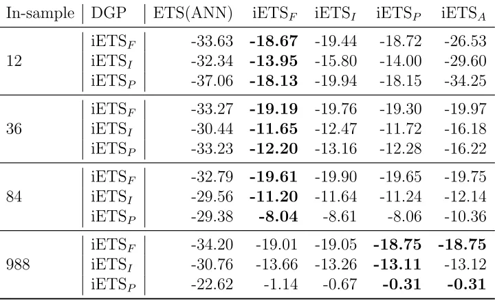
In order to summarise PLS across all the series, we use the arithmetic mean. Higher values of PLS indicate better estimation of the distribution. The results of the simulation are shown in Tables 1 and 2. The first column in both tables shows the number of observations in the sample, and the second column shows the data generating processes used. The other columns show iETS models applied to the data. The continuous iETS models are shown in Table 1, while their integer analogues are summarised in Table 2. The highest values for each sample size and data generating process are shown in bold.
In-sample DGP ETS(ANN) iETSF iETSI iETSP iETSA
12
iETSF -33.63 -18.67 -19.44 -18.72 -26.53
iETSI -32.34 -13.95 -15.80 -14.00 -29.60
iETSP -37.06 -18.13 -19.94 -18.15 -34.25
36
iETSF -33.27 -19.19 -19.76 -19.30 -19.97
iETSI -30.44 -11.65 -12.47 -11.72 -16.18
iETSP -33.23 -12.20 -13.16 -12.28 -16.22
84
iETSF -32.79 -19.61 -19.90 -19.65 -19.75
iETSI -29.56 -11.20 -11.64 -11.24 -12.14
iETSP -29.38 -8.04 -8.61 -8.06 -10.36
988
iETSF -34.20 -19.01 -19.05 -18.75 -18.75
iETSI -30.76 -13.66 -13.26 -13.11 -13.12
[image:27.612.126.486.127.346.2]iETSP -22.62 -1.14 -0.67 -0.31 -0.31
Table 1: PLS values for continuous models applied to simulated data.
where the difference between data produced by different models becomes more substantial.
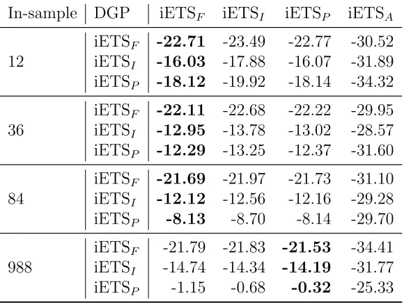
Table 2 shows similar results concerning the performance of intger iETSF, iETSI and iETSP. However the model selection mechanism for integer mod-els does not seem to work for small samples. The important thing to note is that all the integer valued models perform worse than their continuous counterparts on all the samples and all the DGPs. For example, continuous iETSF applied to data generated from fixed probability model with sample size of 84 has PLS of -19.61 (Table 1), while its integer counterpart produced PLS=-21.69 (Table 2). This shows that although the integer valued models are designed to work on this data, they produce less accurate distributions than their continuous analogues. We will investigate this effect further in the next section on real data.
In-sample DGP iETSF iETSI iETSP iETSA
12
iETSF -22.71 -23.49 -22.77 -30.52 iETSI -16.03 -17.88 -16.07 -31.89 iETSP -18.12 -19.92 -18.14 -34.32
36
iETSF -22.11 -22.68 -22.22 -29.95 iETSI -12.95 -13.78 -13.02 -28.57 iETSP -12.29 -13.25 -12.37 -31.60
84
iETSF -21.69 -21.97 -21.73 -31.10 iETSI -12.12 -12.56 -12.16 -29.28
iETSP -8.13 -8.70 -8.14 -29.70
988
iETSF -21.79 -21.83 -21.53 -34.41 iETSI -14.74 -14.34 -14.19 -31.77
[image:28.612.161.451.127.345.2]iETSP -1.15 -0.68 -0.32 -25.33
Table 2: PLS values for integer models applied to simulated data.
Overall we have expected that each of the applied models would perform better on the data generated from the respective processes, but our experi-ment shows that this is not true. The model with fixed probability performs better than all the others on small samples and may be preferred to more complicated ones. However iETSP performed very well in many cases and especially well on large samples. Taking its overall good performance and flexibility, we would recommend it as a basic model for intermittent demand forecasting. The iETSI model did not perform well in our experiment. But this does not mean that it is not applicable at all. It may perform better on time series with slowly increasing probability (for example, with lower vari-ance σ2
q). Finally, we found that integer valued iETS models perform worse than their continuous counterparts.
4.2. Real time series experiment
In order to examine the performance of the proposed intermittent state-space models, we conduct experiment on two datasets.
The second dataset is Royal Air Force data, which contains 5000 real time series (Eaves and Kingsman, 2004). Each of the time series in this dataset has 84 observations. We withheld 12 observations and use them in order to measure forecasting accuracy of tested models.
We have used the same set of models as in Section 4.1 in this experiment and added the following benchmark methods and filters implemented in the
tsintermittent, v2.0 package for R:
1. Hurdle shifted Poisson filter (denoted “HSP”) discussed in Snyder et al. (2012) implemented in hsp() function;
2. Negative Binomial filter (denoted “NegBin”) from Snyder et al. (2012), implemented in the function negbin().
3. TSB method implemented intsb() function;
4. Croston’s method implemented in crost()function; 5. SBA method implemented in crost()function.
We can calculate PLS only for iETS model, HSP and NegBin filters. The last three methods produce expected values only and the distribution of values cannot be estimated correctly for them. So we measure accuracy of point forecasts of all the competing methods and models as well. In order to measure performance of all of them we use the following error metrics, discussed in Kourentzes (2014) and Petropoulos and Kourentzes (2015):
• sME – scaled Mean Error;
• sMSE – scaled Mean Squared Error; • sAPIS – scaled Absolute Periods in Stock.
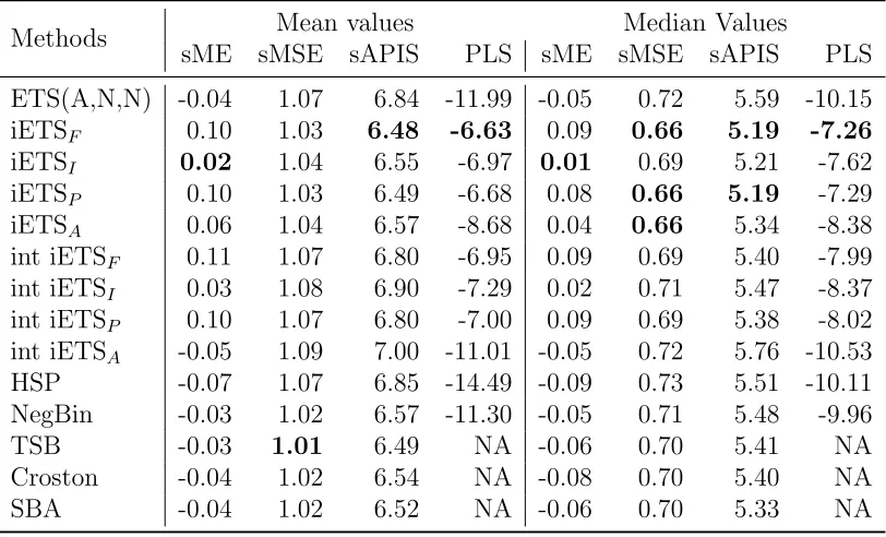
We have calculated mean and median values of these errors across all the series and summarised them in two tables. In cases when data had no vari-ability in-sample and when models produced unrealistic forecasts, PLS re-turned infinite values. So we excluded those cases, when calculating PLS, which left us with 2785 series instead of 3000 in Automotive data and 4365 series instead of 5000 in RAF data.
Methods Mean values Median Values
sME sMSE sAPIS PLS sME sMSE sAPIS PLS
ETS(A,N,N) -0.04 1.07 6.84 -11.99 -0.05 0.72 5.59 -10.15
iETSF 0.10 1.03 6.48 -6.63 0.09 0.66 5.19 -7.26
iETSI 0.02 1.04 6.55 -6.97 0.01 0.69 5.21 -7.62
iETSP 0.10 1.03 6.49 -6.68 0.08 0.66 5.19 -7.29
iETSA 0.06 1.04 6.57 -8.68 0.04 0.66 5.34 -8.38
int iETSF 0.11 1.07 6.80 -6.95 0.09 0.69 5.40 -7.99
int iETSI 0.03 1.08 6.90 -7.29 0.02 0.71 5.47 -8.37
int iETSP 0.10 1.07 6.80 -7.00 0.09 0.69 5.38 -8.02
int iETSA -0.05 1.09 7.00 -11.01 -0.05 0.72 5.76 -10.53
HSP -0.07 1.07 6.85 -14.49 -0.09 0.73 5.51 -10.11
NegBin -0.03 1.02 6.57 -11.30 -0.05 0.71 5.48 -9.96
TSB -0.03 1.01 6.49 NA -0.06 0.70 5.41 NA
Croston -0.04 1.02 6.54 NA -0.08 0.70 5.40 NA
[image:30.612.112.518.126.372.2]SBA -0.04 1.02 6.52 NA -0.06 0.70 5.33 NA
Table 3: Automotive data results.
biased model judging by both mean and median values of sME. The TSB method was more accurate on mean value of sMSE. The differences between the methods and models do not look substantial. As for the PLS, it is worth noting that although the data we deal with is count, the continuous models outperform consistently integer models both in mean and median values. It is also worth pointing out that almost all the iETS models outperform both Hurdle shifted Poisson and Negative Binomial filters of Snyder et al. (2012) in the majority of measures.
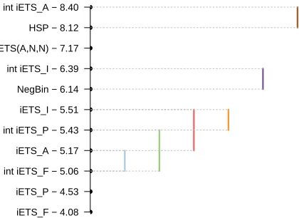
In order to determine if the differences between the models are statistically significant, we have conducted a Nemenyi test (Demˇsar, 2006) on PLS values. The results of this test are shown in Figure 1. The ranking was done so that the model with the highest PLS would have the score of 1 and the model with the lowest PLS would have the score of 10. The Y-axis in Figure 1 shows average ranks for each of the models. The vertical lines in the figure show the groups of models, in which the difference between the ranks is statistically insignificant. The significance level used in this experiment is 5%.
iETS_F − 4.08 iETS_P − 4.53 int iETS_F − 5.06 iETS_A − 5.17 int iETS_P − 5.43 iETS_I − 5.51 NegBin − 6.14 int iETS_I − 6.39 ETS(A,N,N) − 7.17 HSP − 8.12 int iETS_A − 8.40
Figure 1: Nemenyi test for models applied to automotive data.
The difference between integer iETSF, continuous iETSA with model selec-tion and integer iETSP is statistically insignificant. The HSP filter performed significantly worse than all the models outperforming only the integer iETSA with model selection. At the same time, the Negative Binomial filter per-forms significantly better than the Posson filter (which agrees with the finding of Snyder et al., 2012) and some of the iETS models. It is at least as good as the integer iETSI model, but significantly worse than the integer iETS with fixed and TSB probabilities. It also performed worse than all the other continuous iETS models. It is also worth pointing out that the model se-lection in case of integer model does not perform well. So we would advise either using continuous iETS with model selection instead or to use iETSF or iETSP for this data.
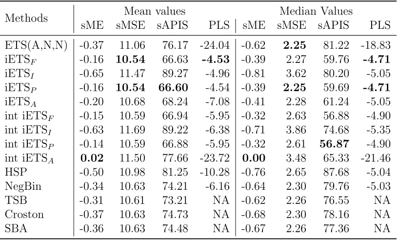
The results of the experiment for the Royal Air Force data are shown in Table 4.
Methods Mean values Median Values
sME sMSE sAPIS PLS sME sMSE sAPIS PLS
ETS(A,N,N) -0.37 11.06 76.17 -24.04 -0.62 2.25 81.22 -18.83
iETSF -0.16 10.54 66.63 -4.53 -0.39 2.27 59.76 -4.71
iETSI -0.65 11.47 89.27 -4.96 -0.81 3.62 80.20 -5.05
iETSP -0.16 10.54 66.60 -4.54 -0.39 2.25 59.69 -4.71
iETSA -0.20 10.68 68.24 -7.08 -0.41 2.28 61.24 -5.05
int iETSF -0.15 10.59 66.94 -5.95 -0.32 2.63 56.88 -4.90
int iETSI -0.63 11.69 89.22 -6.38 -0.71 3.86 74.68 -5.35
int iETSP -0.14 10.59 66.88 -5.95 -0.32 2.61 56.87 -4.90
int iETSA 0.02 11.50 77.66 -23.72 0.00 3.48 65.33 -21.46
HSP -0.50 10.98 81.25 -10.28 -0.76 2.65 87.68 -5.04
NegBin -0.34 10.63 74.21 -6.16 -0.64 2.30 79.76 -5.03
TSB -0.31 10.61 73.21 NA -0.62 2.26 76.55 NA
Croston -0.37 10.63 74.73 NA -0.68 2.30 78.16 NA
[image:32.612.112.520.125.372.2]SBA -0.36 10.63 74.48 NA -0.67 2.26 77.36 NA
Table 4: Royal Airforce data results.
which has the least biased forecasts measured by both mean and median sME. The worst performing model (in terms of sME, sMSE and sAPIS) on this dataset is iETSI (both continuous and integer versions). It even per-forms worse than Croston’s method, which points to the differences at the estimation of parameters. This may be explained by the maximum likeli-hood estimation of parameters of the model leading to less accurate point forecasts on this dataset than in case with the simple estimation methods (implemented in the tsintermittent package). The HSP filter performed similarly to how it performed on a previous dataset, this time slightly outper-forming ETS(A,N,N) and outperoutper-forming iETSI model. As for the Negative Binomial filter, it performed better than HSP in all the measures (once again agreeing with Snyder et al., 2012). Finally, the model selection mechanism in case of integer iETS model does not seem to work well.
Following the same procedure as with automotive data, we have con-ducted a Nemenyi test with the results shown in Figure 2.
iETS_P − 3.66 int iETS_P − 3.92 iETS_F − 4.53 int iETS_F − 4.77 iETS_A − 4.83 NegBin − 5.12 iETS_I − 6.47 int iETS_I − 6.79 HSP − 7.00 ETS(A,N,N) − 8.26 int iETS_A − 10.64
Figure 2: Nemenyi test for models applied to Royal Air Force data.
for the HSP filter, it was the third worst model in the comparison, performing similar to the integer iETSI model. Finally, Negative Binomial filter outper-formed both iETSI models and HSP, but it could not produce as accurate forecasts as iETSF and iETSP.
As can be seen from this experiment the proposed intermittent state-space models perform very well and can be applied to real life problems. The iETSP model seems to be the most robust of all of them. Although we know that the data we deal with is count and that the continuous model is wrong in this case, we found that it is still useful.
5. Conclusions
This paper was focused on the ETS(M,N,N) model and the intermittent equivalent of this model was called iETS(M,N,N). Firstly we have proposed a simple state-space model with fixed probability (denoted as “iETSF”), which is very easy to estimate and use. We have shown that Croston’s method has an underlying statistical model (denoted as “iETSI”), which allows the calculation of conditional expectation and variance. After that we have shown that the TSB method also has an underlying statistical model (denoted as “iETSP”), which allows estimation of the model parameters. We have also derived the likelihood functions for all the iETS models, which allow not only obtaining efficient and consistent estimates of parameters, but also selecting between several state-space models. This also includes selecting between intermittent and non-intermittent models, thereby simplifying the forecasting process. We have shown that the forecasts produced by iETSI and iETSP correspond to the conditional median of demand sizes rather than the mean, which in case of intermittent data is a useful property. We have also proposed an algorithm of parametric prediction intervals construction using the proposed intermittent state-space model. Finally, we developed integer counterparts of iETS models which address the issue of count data modelling.
We conducted several experiments on simulated and real data. The sim-ulation that we have conducted shows several interesting results. First, it seems that integer iETS models do not perform as accurately as their con-tinuous counterparts. Second, iETSF and iETSP work very well on small samples of data generated from different iETS models. Third, iETSP works better than the other models on large samples, being able to produce the most accurate forecasts for all the DGPs. Fourth, iETS with model selec-tion improves its performance with an increasing sample size. We argue that iETSP should be preferred to other models on small samples as a more robust and more flexible model. It is able to produce accurate forecasts on a wide variety of time series from different data generating processes.
Finally, the experiment on automotive data and on data from the Royal Air Force shows that the proposed approach is applicable to real life supply chain problems and that the proposed models perform very well on different datasets. They outperformed the existing forecasting methods and several filters previously proposed in the literature. iETSP generally was one of the best forecasting models on both data sets. We would advise it as one of the most robust models, applicable to wide variety of series.
model, which underlies the two intermittent demand forecasting methods studied in the paper (Croston’s and TSB). We simplified the notation for this model in the paper. However, we propose a more detailed one, which acknowledges the flexibility of the proposed approach and the fact that both demand sizes and demand occurrence parts may have their own ETS models (potentially with exogenous variables). So, the model with demand intervals, discussed in the paper can be denoted as iETS(M,N,N)(M,N,N)I, where the letters in the first brackets indicate the type of ETS model for demand sizes and the letters in the second ones indicate the type of ETS model used for demand intervals. Using this notation, new types of models can be stud-ied in future research. For example, model with additive trend in demand sizes and multiplicative trend in time varying probability can be denoted as iETS(M,A,N)(M,M,N)P. This allows extending the Hyndman et al. (2008) taxonomy and opens new avenues for the research.
It is also worth mentioning that the approach of intermittent state-space modelling allows using (for both demand sizes and demand occurrence parts of the model) ETS, ARIMA, regression models or diffusion models, which could be applied to a wide range of time series (not limited with intermittent demand). Studying properties of such models would be another large area of research. The other possible direction of research is the development of a new model for demand occurrence, as both Croston’s and TSB mechanisms have their own flaws. Finally, in order to show the connections between the methods and the models, we assumed throughout this paper that demand occurrence and demand size parts are independent. This could be modified in a new model using the state-space approach discussed in the paper.
Appendix A. Properties of ETS(M,N,N) model
the parameters of the normal distribution:
E(1 +t) = exp
µ+
σ2 2
. (A.1)
Even if µ = 0 in the model (12), σ2 is not equal to zero. If µ is close to −σ2
2 , then the sample path of ETS(M,N,N) will converge almost surely to zero as discussed in Akram et al. (2009), because the expected value of (1 +t) will be close to one in this case, meaning that E(t) tends to zero and E(1 +αt) tends to one. In the other case, when µ <−σ
2
2 , the sample path will converge to zero asymptotically, because E(1+t) becomes less than one, making E(1 +αt) <1 as well, leading to diminishing values of the level of time series lt. Finally, when µ > −σ
2
2 the sample path will asymptotically diverge from zero, because E(1 +αt)>1, which causes growth of level. This is an important property, because it implies that with different values of µ and σ2
the model will behave differently.
The properties of the log-normal distribution and the multiplicative model also restrict the smoothing parameter with the interval [0, 1]. Assuming that the smoothing parameter is always positive, the inequality (1+t)>0 implies that:
t >−1
αzt>−αz 1 +αzt>1−αz
(A.2)
The ETS(M,N,N) model makes sense only when 1 +αzt>0. So, if αz >1, then 1+αztmay become negative, which breaks the model, because the level may become negative. The model however still makes sense for boundary values of αz: when αz = 0, the level is not updated, while in the case of
αz = 1, the level has the dynamics of a random walk process. The condition
αz ∈[0,1] is rather restrictive, because there may be some cases when even with αz > 1 the value of (1 +αzt) will be greater than zero. However it guarantees that the level of time series is always positive whatever the error value is.
Appendix B. Likelihood function for iETS(M,N,N)
The likelihood function for the log-normal distribution L(θ, σ2
the parameters of the model, µz,t|t−1 is the conditional mean and σ2 is the variance of one-step-ahead forecast error for demand sizes.
There are two cases for the intermittent demand model: when demand occurs and when it does not. In the former case, the probability of obtaining the value yt is equal to:
P(yt|θ, σ2, ot= 1) =L(θ, σ2|yt, ot= 1) =ptL(θ, σ2|zt). (B.1) In the latter case it is just equal to the probability of non-occurrence:
L(θ, σ2
|yt, ot= 0) = (1−pt). (B.2) The likelihood function for all the T observations, which include T0 cases of non-occurrence and T1 cases of demand occurrence, is then:
L(θ, σ2|Y) = Y ot=1
ptL(θ, σ2|zt)
Y
ot=0
(1−pt), (B.3)
where Y is the set of all the variables yt. Taking the logarithm of (B.3), we obtain:
`(θ, σ2
|Y) = −
X
ot=1
log(zt) + 1
2log(2πσ 2 ) +
1 2
logzt−logµz,t|t−1
2 σ2 ! +X ot=1
log(pt) + X ot=0
log(1−pt)
.
(B.4) The varianceσ2
can be estimated using this likelihood (by taking the deriva-tive of (B.4) with respect to σ2
and equating it to zero) and is equal to: ˆ
σ2 = 1
T1
X
ot=1
log2(1 +t), (B.5)
where log(1 +t) = logzt−logµz,t|t−1. In addition, the probability pt is also not known and needs to be substituted by the estimated value ˆpt. All of this leads to the following concentrated log-likelihood:
`(θ,σˆ2
|Y) = −
T1
2 log(2πe) + log(ˆσ 2 )
−X
ot=1
log(zt)
+X
ot=1
log(ˆpt) +X ot=0
Appendix C. Conditional variance for iETSF
Knowing that σ2
o,t+h|t = p(1−p) for a Bernoulli process and inserting it in (11) leads to:
σy,t2 +h|t=p(1−p)σ2z,t+h|t+p(1−p)µ2z,t+h|t+p2σ2z,t+h|t, (C.1) which then can be simplified to:
σ2y,t+h|t =pσz,t2 +h|t+p(1−p)µ2z,t+h|t. (C.2)
Appendix D. Likelihood function for iETSI
In order to derive the likelihood for iETSI model, the probability density function for pt = 1+1qt needs to be derived. This can be done, taking into account that qt has a log-normal distribution, using the formula:
fy(y) =
dyd g−1(y)
fx(g−1(y)), (D.1)
where y = g(x), x = g−1(y) is the inverse function of y and fx(·) is the density function of x. qt can be reformulated as qt= 1−ptpt, the differential of which is equal to −1
p2
t. Inserting this in (D.1), the density function ofpt is:
f(pt|θq) = 1
p2 t
1 1−pt
pt
p
2πσ2 q
e−
(log(1−ptpt)−logµq,t|t−1)2
2σq2 , (D.2)
which becomes:
f(pt|θq) = 1
pt(1−pt) 1
p
2πσ2 q
e−
(log(1−pt)−log(pt)−logµq,t|t−1)2
2σ2q , (D.3)
where θq is the vector of parameters relating to the occurrence part of the model. The probability of having an occurrence is now a compound with the following density function:
f(ot =k|θq) =
Z 1
0
where k = 1, when demand occurs and k = 0 otherwise. The density func-tions (D.4) and (D.3) can now be inserted in the general likelihood function (B.3), discussed in Appendix B. However there is no point in doing so, and it is sufficient to note that maximisation of the likelihood (B.3) means auto-matically the maximisation of (D.3). And if we make the substitutionpt= q1t in (D.3) we will have the likelihood function for qt based on the log-normal distribution. This means that the estimation of iETSI model can be done in two steps: first the occurrences part should be estimated via maximisation of the likelihood function forqt, then the general model can be estimated using (B.3) and the expected values of probabilities from iETSI model. This also demonstrates the connection between the optimisation procedure on demand intervals level and on the level of the model as a whole.
Appendix E. Likelihood function for iETSP
The likelihood function for iETSP resembles the likelihood of the general iETS model. The only difference is in the probability of occurrences. So the concentrated log-likelihood can be written as:
`(θ, σ2
|Y) =−
T1
2 log(2πe) + log(ˆσ 2 )
−X
ot=1
log(zt)
+X
ot=1 log
B(ot+at,1−ot+bt) B(at, bt)
+X
ot=0 log
B(ot+at,1−ot+bt) B(at, bt)
,
(E.1) where B(a,b) is the Beta function with parameters a and b. The likelihood (E.1) can be simplified to (taking TSB restriction of at+bt = 1):
`(θ, σ2
|Y) =−
T1
2 log(2πe) + log(ˆσ 2 )
−X
ot=1
log(zt)
+X
ot=1 log
B(1 +at,1−at) B(at,1−at)
+X
ot=0 log
B(at,1 + 1−at) B(at,1−at)
.
(E.2)
Now we should recall two important properties of the Beta function. They are:
B(1 +a, b) =aB(a, b) a+b
B(a,1−a) = π sin(πa).
Using these properties, it can be shown that: B(1 +at,1−at)
B(at,1−at)
=at
B(at,1−at)
at+ 1−at
sin(πat)
π =at π
sin(πat)
sin(πat)
π =at.
(E.4) Similarly it can be shown that:
B(at,1 + 1−at) B(at,1−at)
= 1−at. (E.5)
This means that the log-likelihood function for this model is:
`(θ, σ2
|Y) = −
T1
2 log(2πe) + log(ˆσ 2 )
−X
ot=1
log(zt)
+X
ot=1
log(at) + X ot=0
log(1−at) . (E.6)
However at is unknown and thus should be estimated using ETS(M,N,N). This gives us the following final concentrated log-likelihood:
`(θ,σˆ2
|Y) = −
T1
2 log(2πe) + log(ˆσ 2 )
−X
ot=1
log(zt)
+X
ot=1
log(la,t−1) +
X
ot=0
log(1−la,t−1)
, (E.7)
Appendix F. Conditional values of iETS(M,N,N)
If we rewrite the demand size part of the general intermittent state-space model (12) in logarithms:
yt=ot(loglz,t−1 + log (1 +t))
loglz,t= loglz,t−1+ log(1 +αzt) (F.1) then the measurement equation for yt+h can be written as:
yt+h =ot+hexp loglz,t+ h−1
X
j=1
log(1 +αzt+h−j) + log(1 +t+h)
!
. (F.2)
The part inside the exponent in (F.2) will have a normal distribution if (1 +t) has a log-normal distribution. The conditional expectation and vari-ance of that part will then be:
˜
µz,t+h|t= loglz,t ˜
σ2
z,t+h|t=σ2
1 +Phj=1−1σ2 α