Blinded versus unblinded estimation of a correlation coefficient to inform interim design adaptations

warwick.ac.uk/lib-publications

Original citation:

Kunz, Cornelia, Stallard, Nigel, Parsons, Nicholas R., Todd, Susan and Friede, Tim. (2016)

Blinded versus unblinded estimation of a correlation coefficient to inform interim design

adaptations. Biometrical Journal.

Permanent WRAP URL:

http://wrap.warwick.ac.uk/80114

Copyright and reuse:

The Warwick Research Archive Portal (WRAP) makes this work of researchers of the

University of Warwick available open access under the following conditions.

This article is made available under the Creative Commons Attribution 4.0 International

license (CC BY 4.0) and may be reused according to the conditions of the license. For more

details see:

http://creativecommons.org/licenses/by/4.0/

A note on versions:

The version presented in WRAP is the published version, or, version of record, and may be

cited as it appears here.

Blinded versus unblinded estimation of a correlation coefficient to

inform interim design adaptations

Cornelia U. Kunz∗,1_{, Nigel Stallard}1_{, Nicholas Parsons}1_{, Susan Todd}2_{,andTim Friede}3 1 _{Warwick Medical School, University of Warwick, Gibbet Hill, Coventry, CV4 7AL, UK} 2 _{Department of Mathematics and Statistics, University of Reading, Whiteknights, PO Box 220,}

Reading, RG6 6AX, UK

3 _{Department of Medical Statistics, University Medical Center Goettingen, Humboldtallee 32,}

D-37073 Goettingen, Germany

Received 31 October 2015; revised 20 June 2016; accepted 4 July 2016

Regulatory authorities require that the sample size of a confirmatory trial is calculated prior to the start of the trial. However, the sample size quite often depends on parameters that might not be known in advance of the study. Misspecification of these parameters can lead to under- or overestimation of the sample size. Both situations are unfavourable as the first one decreases the power and the latter one leads to a waste of resources. Hence, designs have been suggested that allow a re-assessment of the sample size in an ongoing trial. These methods usually focus on estimating the variance. However, for some methods the performance depends not only on the variance but also on the correlation between measurements. We develop and compare different methods for blinded estimation of the correlation coefficient that are less likely to introduce operational bias when the blinding is maintained. Their performance with respect to bias and standard error is compared to the unblinded estimator. We simulated two different settings: one assuming that all group means are the same and one assuming that different groups have different means. Simulation results show that the na¨ıve (one-sample) estimator is only slightly biased and has a standard error comparable to that of the unblinded estimator. However, if the group means differ, other estimators have better performance depending on the sample size per group and the number of groups.

Keywords: Blinded; Correlation; Covariance; Estimation; Unblinded.

1

Introduction and motivation

The traditional approach to conducting a confirmatory clinical trial is to calculate a fixed sample size in advance of the study. This sample size usually depends on a specified significance level and power but also on other parameters such as variances, mean values, or response rates. While the significance level and power are set by the researcher, the other parameters are usually estimates obtained from previous trials. However, situations occur where these parameters cannot be estimated or can be estimated only with considerable uncertainty at the planning stage of the trial. Designs allowing a re-assessment of the initial sample size during an ongoing trial have become increasingly popular. Several approaches to estimate the variance in an ongoing trial have been suggested and their performance has been studied. One approach is the common pooled variance estimator that is often used for sample size

∗_{Corresponding author: e-mail:[email protected], Phone:+44-1524-595-233}

re-estimation (see, e.g. Wittes and Brittain, 1990; Birkett and Day, 1994; Coffey and Muller, 1999; Denne and Jennison, 1999; Wittes et al., 1999; Zucker et al., 1999; Kieser and Friede, 2000; Coffey and Muller, 2001; Miller, 2005). This estimator requires unblinding of the treatment group at the time of the interim analysis. As blinding of patients, investigators and the trial team is important in clinical trials to avoid bias (see, e.g. International Conference on Harmonisation of Technical Requirements for Registration of Pharmaceuticals for Human Use (ICH), 1998), regulatory guidelines on adaptive designs encourage the use of blinded methods (European Medicines Agency (EMEA) - Committee for Medicinal Products for Human Use (CHMP), 2007; Food and Drug Administration (FDA), 2010). As a consequence, estimators based on the blinded data set have been proposed. Bristol and Shurzinske (2001) suggested the total variance or one-sample variance estimator that is unbiased if there are no group differences but otherwise overestimates the within group variance. In order to reduce bias, Gould and Shih (1992) and Zucker et al. (1999) proposed correction methods for the one-sample variance estimator by subtracting a between-group variance term from the one-sample estimator based on an assumed treatment effect. Xing and Ganju (2005) proposed an unbiased estimator based on the blinded data that utilises information about the randomisation block size. They later extended their method to the situation of covariates (Ganju and Xing, 2009). These blinded estimators were recently compared with regard to bias and variance by Friede and Kieser (2013). A review of the various sample size re-estimation procedures can be found in Friede and Kieser (2006).

In some cases the sample size required can depend on the correlation between different measurements in addition to the variance. However, often there is very little information available on the correlation at the planning stage of a clinical trial. Hence, investigators might want to estimate the correlation in an ongoing trial.

In this paper, we develop and compare estimators for the covariance and the correlation based on blinded data obtained at an interim analysis. The estimators are compared with respect to their bias and their standard error.

In the remainder of this section we provide a brief overview of situations where the value of the correlation is required and it might be beneficial to obtain an estimate of this based on interim data. The rest of our paper is organised as follows: Section 2 introduces the notation used in the paper and describes the different estimators we have considered. Our findings are summarised in Section 3 and we close the paper with the discussion in Section 4.

1.1 Multiple primary endpoints

for at least one of the endpoints under consideration. Li and Mehrotra (2008), for example, develop a method where the significance level for a second primary endpoint depends on the observedp-value for the first one. Their approach also depends on the correlation between the endpoints.

1.2 Multiple short-term surrogate endpoints

Other situations where the correlation between measurements can be of importance for the perfor-mance of a method include the use of short-term (surrogate) secondary endpoints to inform decisions in an ongoing trial. Galbraith and Marschner (2003) discuss interim analyses for clinical trials where an endpoint is observed repeatedly during follow-up, with the last observation being considered the primary endpoint. They show that the correlation between the measurements taken at different time points can be exploited in order to increase the precision of the estimate of the primary endpoint effect. Todd and Stallard (2005) describe a method for adaptive seamless phase II/III designs where a secondary endpoint is incorporated into the trial design in order to select the most promising treat-ment at an interim analysis (see also Stallard, 2010; Kunz et al., 2015). Furthermore, Kunz et al. (2014) developed an approach to select the most promising treatment based on interim analysis data incorporating a short-term endpoint. The last methods depend on the ability to obtain an unbiased estimate of the correlation coefficient in an ongoing trial, often based on very little data.

2

Statistical methods

2.1 Notation

LetG≥2 denote the number of arms within a multi-arm, randomised, controlled, double-blind trial and letn_gdenote the number of patients in group g(g=1. . .G) for which data are available with

n=G_g=1n_g. Furthermore, letG(i)denote a function indicating group membership for patienti, that is withG(i)=gif patientiis in groupg. Assume that in each of theGgroups two measurements (x_i

andy_i) per patient are taken that follow a bivariate normal distribution with

X_i Y_i ∼N ⎛ ⎜ ⎝

μx_G(i)

μy_G(i) ,

⎛ ⎜ ⎝

σ2

x_G(i) ρσx_G(i)σy_G(i)

ρσx_G(i)σy_G(i) σy2_G(i)

⎞ ⎟ ⎠ ⎞ ⎟ ⎠.

Note, that we assume the correlation to be independent of the group, that is the correlation betweenX

andYis the same within each groupg. Furthermore, whileμ_x

gandμygdenote the unknown population

parameters of groupg, for some methods described below it is necessary to specify values for these parameters that are assumed in order to estimate the covariance or correlation. Letμ˜_x

gandμ˜ygdenote

these assumed values withμ˜_x

g=μxg+δxg,μ˜yg=μyg+δyg,μx= G

g=1

n_g

nμx_g,μy=

G g=1

n_g

nμy_g,δx=

G g=1

n_g

nδx_g,δy=

G g=1

n_g

nδy_g,μ˜x=

G g=1

n_g

nμ˜x_g, andμ˜y =

G g=1

n_g nμ˜y_g.

We mainly focus on block randomisation but also include results for simple randomisation (Altman and Bland, 1999) for one blinded estimator. LetB(i)denote a function indicating block membership for patienti, that is withB(i)=bif patientiis in groupb.

2.2 Time of the analysis

Table 1 Proposed estimators for the covariance.

Block randomisation Unblinded

Pooled cov_pool=1

n

G g=1

n_g

ng−1 i:G(i)=g(xi− ¯xg)(yi− ¯yg)

Blinded

Na¨ıve cov_na¨ıve= _n−1₁n_i=1(x_i− ¯x)(y_i− ¯y)

Based on Xing and Ganju cov_XG= _n(BB₋₁₎B_{b=1 i:B(i)=b}(x_i− ¯x) _i:B(i)=b(y_i− ¯y)

Based on Zucker et al.

Usingx¯,y¯ cov_Z1=n−_n1cov_na¨ıve−G_g=1ng

nμ˜x_gμ˜y_g+ ¯xy¯

Usingμ˜_x,μ˜_y cov_Z2=cov_na¨ıve−G_g=1 ng

n−1μ˜x_gμ˜y_g+n−n1μ˜xμ˜y

Simple randomisation

Blinded cov_sr=_n−1₁n_i=1(x_i− ¯x)(y_i− ¯y)

randomisation, the number of patients per group,n_g, is also fixed. If simple randomisation is used only the total number of patients,n, is fixed whilen_gcan vary.

2.3 Estimation of the covariance

Our ultimate aim is to estimate the correlationρ. However, we start by focusing on estimating the covariance betweenXandY. Table 1 lists the six different estimators we have investigated. In order to calculate the pooled covariancecov_pool, we need to unblind the data. We then calculate the covariance within each group and take a “weighted average” across the groups. If we do not unblind the data, four different estimators for the covariance can be defined. The “na¨ıve” estimatorcov_na¨ıveis obtained by calculating the covariance for the whole data set, that is treating the data as if they were obtained from just one group. This method can always be applied, hence, we present results not only for block randomisation but also for simple randomisation (cov_sr).

The other estimators all require block randomisation. Xing and Ganju (2005) developed an estimator for the variance of an endpoint in an ongoing blinded trial. Their estimator uses the enrollment order of subjects and the randomisation block size to estimate the variance. We extend their method to allow for estimation of the covariance (cov_XG) and different sample sizes, variances, and correlations within each group. Zucker et al. (1999) also propose an estimator for the variance based on blinded data. Their estimator incorporates assumptions about the differences in the means between the different groups. Again, we extend their method to allow for estimation of the covariance and more than two groups as well as different variances, sample sizes, and correlations within each group. We present results for two different versions of this estimator: the first one (cov_Z1) is based on the estimated overall means for the two endpointsx¯andy¯. The second one (cov_Z2) is based on the assumed overall means for the two endpointsμ˜_xandμ˜_y.

3

Results

3.1 Analytical expressions for the expected values of estimators for the covariance

Table 2 Expected values of the estimators for the covariance.

Block randomisation Unblinded

Pooled E[cov_pool]=G_g=1ng

nρσx_gσy_g

Blinded

Na¨ıve E[cov_na¨ıve]=G_g=1 ng

nρσx_gσy_g+ n n−1

G g=1

n_g

nμx_gμy_g−μxμy

Based on Xing and Ganju E[cov_XG]=G_g=1ng

nρσx_gσy_g

Based on Zucker et al.

Usingx¯,y¯ E[cov_Z1]=G_g=1ng

nρσx_gσy_g−

G g=1

n_g n

μx_gδy_g+μy_gδx_g+δx_gδy_g

Usingμ˜_x,μ˜_y E[cov_Z2]=G_g=1ng

nρσx_gσy_g−

G g=1

n_g n−1

μx_gδy_g+μy_gδx_g+δx_gδy_g

+ n

n−1(μxδy+μyδx+δxδy)

Simple randomisation

Blinded E[cov_sr]=G_g=1ng

nρσx_gσy_g+

G g=1

n_g

nμx_gμy_g−μxμy

If we assume equal variancesσ2

x_gandσy2_gwithin each groupg, we see that only two estimators for the

covariance are unbiased: the pooled estimatorcov_pool(based on the unblinded data) and the estimator based on Xing and Ganju (cov_XG) as the expected value for both simplifies toρσ_xσ_ywithσ_x=σ_x

gand σy=σy_g forg=1. . .G. With equal variances, the na¨ıve estimatorscovna¨ıve andcovsr are unbiased if

μx_gandμy_gare 0 forg=1. . .G. The estimators based on Zucker et al. are both unbiased ifδx_g=0

andδ_y

g=0 for allg=1. . .G. However, the second estimatorcovZ2is also unbiased if a much weaker

condition is fulfilled, that is as long asδ_x

g=δxandδyg=δyforg=1. . .Gholds true.

3.2 Application to real data example

Wilcock et al. (2000) report the outcome of a randomised controlled trial of galantamine in patients with mild to moderate Alzheimer’s disease. Two different dose levels (24 and 32 mg) were tested against placebo. The primary endpoint was the score on the 11 item cognitive subscale of the Alzheimer’s disease assessment scale measured after 6 months. Wilkinson et al. (2001) also report the outcome of a randomised trial of galantamine in patients with Alzheimer’s disease. However, they compared three dose levels (18, 24 and 36 mg) to placebo. They used the same primary endpoint but measured after 12 weeks. Wilkinson et al. also report that an interim analysis was carried out after approximately 20 patients per group had completed assessment.

So, in total, there were four treatment groups (dose levels 18, 24, 32 and 36 mg) and the placebo group and two different outcome measures. In such a situation, we might want to use an adaptive seamless Phases II/III design with treatment selection at interim as described by, for example, Todd and Stallard (2005). However, as the method depends on the correlation between the endpoints (see Kunz et al., 2015), we might want to estimate the correlation within the ongoing trial.

Table 3 Parameter settings for the simulation study.

Example 1 Example 2

g μ_x μ_y δ_x δ_y σ_x σ_y μ_x μ_y δ_x δ_y σ_x σ_y

1 0 0 0.1 0.5 1 1 0 0 0.1 0 1 1

2 0 0 0.1 0.5 1 1 0.25 0.25 0.1 −0.125 1 1

3 0 0 0.1 0.5 1 1 0.5 0.5 0.1 −0.25 1 1

4 0 0 0.1 0.5 1 1 0.75 0.75 0.1 −0.375 1 1

5 0 0 0.1 0.5 1 1 1 1 0.1 −0.5 1 1

ρ −0.8, 0,+0.8

G 2, 3, 5

n_g 6, 24

B 2, 3, 6 (ifn_g=6) and 2, 3, 4, 6, 8, 12, 24 (ifn_g=24)

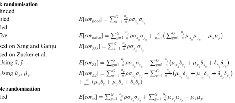
Figure 1 Mean (±s.e.) for the estimate of the correlation coefficient.

Figure 1 shows the results for the real data example. The two scatter plots show examples for how the data might look at the time of the interim analysis. Different markers are used for the different groups. Note that due to the relatively large standard deviation (compared to the relatively small difference between the means) without the different markers, we would not be able to distinguish between the different groups.

For a sample size ofn_g=6, we see that all estimators yield a correlation estimate of about 0.8 except for the estimator based on Xing and Ganju that yields an estimate of 0.76. The latter also has the largest standard error (s.e. 0.22) while the other estimators have a standard error between 0.07 and 0.10.

3.3 Simulation-based estimates for the expected values of estimators for the correlation coefficientρ

In order to obtain a better overview of the properties of the estimators, we simulated data for two examples with different parameter settings that are given in Table 3. For the first example we assumed that all groups have the same meansμ_x

gandμyg, which, without loss of generality, were both set to 0.

This setting reflects a scenario where the null hypothesis would be true. For the estimators based on the work of Zucker et al. we assumed thatδ_x=0.1 andδ_y =0.5 for all groups. For the second example, we assumed different means and differentδ_yfor different groups. For both examples, data were simulated for three different values ofρ, for three different values ofGand for two different values ofn_g. All variances are taken to be equal to 1. For the estimator based on Xing and Ganju, we also considered different values forBdepending on the sample sizen_g. For each scenario considered we simulated data between 10,000 and 3,000,000 times (depending on how stable the results for the standard error were). For each simulated dataset, we estimated the covariance and the variances using one of the methods described above. Note that the variances are a special case of the covariance , that is in general

VAR[X]=cov[X,X]. Hence, the variances can be obtained using the estimators in Table 1 replacing either y with x (to obtain the variance ofX) orx with y (to obtain the variance ofY). We then calculated the correlationrusingr= ˆρ= ˆcov/(σˆ_xσˆ_y).

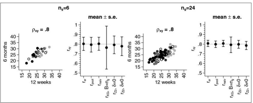
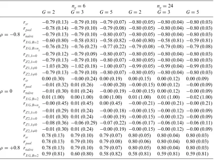
Figure 2 shows the results for Example 1. Results forr_Z1 were omitted in the figure as they were often highly biased. They can still be found in Table A.1 in the Appendix. In the following we will only discuss the results for the other estimators.

The left-hand side of the figure shows schematic examples of the scatter plots for the scenarios considered. The right-hand side shows the results for the correlation estimators for different sample sizes n_g and different numbers of groups G. The upper panel shows the results for ρ= −0.8, the middle panel shows the results forρ=0 and the bottom panel shows the results forρ= +0.8. For each method we present the mean and the standard error (s.e.). Overall, nearly all estimators are unbiased except for the estimator based on Xing and Ganju. For a correlation ofρ= ±0.8, we obtain

r_XG= ±0.6 ifB=2. The expected value of the estimator is not affected by the number of groupsG

nor by the sample sizen_g. The only parameter that affects the results for this particular estimator is the number of blocksB. IfB=n_g, the estimator is less biased and has a smaller standard error that can be seen by comparing the results forn_g=6 withn_g=24. Ifρ= ±0.8,n_g=6 andB=n_g=6, the estimated correlation isr_XG= ±0.76(s.e.±0.23)while ifn_g=24 andB=n_g=24, the estimated correlation isr_XG=0.79(s.e.±0.08). Ifρ =0, the estimator based on Xing and Ganju is unbiased but still has the largest standard error irrespective of the sample sizes, the number of groups or the number of blocks.

All other estimators lead to very similar results. In all cases the estimators are either unbiased or the bias is very small compared to the standard error. The standard errors depend on the sample sizes and the number of groups, with larger sample sizes and more groups leading to smaller standard errors. It might be noteworthy that the standard error also depends on the correlationρ, withρ=0 leading to the largest standard error for all estimators.

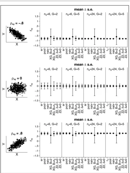
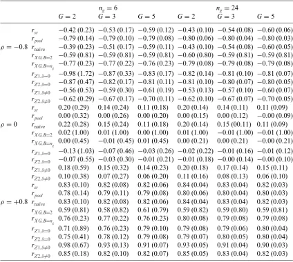
The situation changes if the group means are different as can be seen from Figure 3 (again results forr_Z1are omitted from the figure, but are included in the Appendix in Table A.2). Now, nearly all estimators are biased except for the “pooled” one which requires unblinding. Largest bias occurs for the na¨ıve estimator forρ= −0.8,n_g=6 andG=2. In this case, the average estimated correlation isr_na¨ıve = −0.41 with a standard error of 0.23. While the bias gets smaller if the number of groups increases, the sample size per group does not have much impact. For example, for ρ= −0.8 the estimated correlation is−0.41 (−0.43) forG=2 andn_g=6 (n_g=24),−0.53 (−0.54) forG=3 and

The estimator based on the work of Xing and Ganju is less biased than the na¨ıve estimator. However, especially if data for only two blocks is available, the standard error is very large. Forρ= ±0.8 we obtain a standard error of about 0.80 and forρ =0 we get 1. Hence, if we calculate a 95% confidence interval it would actually span the entire range of possible values forρfrom−1 to 1. Results for this estimator improve whenB=n_g. However, large standard errors can still occur.

The estimator based on the work by Zucker et al. is also biased, even ifδ_x andδ_y are 0, that is, even if we guess the true population means correctly, we still under- or overestimate the correlation. For example, forn_g=6 andG=2, we getr_Z2= −0.88 (forρ= −0.8),r_Z2= −0.08 (forρ=0), and

r_Z2=0.76 (forρ= +0.8). While results improve for larger sample sizes and more groups, the estimator still depends onδ_xandδ_y, that is on the ability to correctly “guess” the differences between the group means. It also should be noted that forn₆=6 andG=2, the standard error of the estimators based on the work of Zucker at al. can be quite substantial and sometimes even larger than the one for the estimator based on Xing and Ganju forB=2. Further results for other scenarios can be found in the online Supporting Information.

4

Discussion

In this paper, we have considered a number of estimators for the correlation coefficient based on blinded and unblinded data to inform interim decisions in flexible designs and have compared their performance. We have mainly focused on block randomisation and blinded estimators.

Unsurprisingly, the unblinded estimator is only slightly biased and tends to have the smallest standard error in all investigated settings. However, it requires unblinding, whereas maintaining the blind is considered to be one of the most important techniques (together with randomisation) to eliminate or minimise bias (International Conference on Harmonisation of Technical Requirements for Registration of Pharmaceuticals for Human Use (ICH), 1998).

Under the null hypothesis, the na¨ıve estimator performs best out of all estimators based on blinded data. Furthermore, it requires no assumptions and no information other than the data for the two variables under consideration. Yet, its performance is similar to the unblinded estimator for this scenario. However, under the alternative, the bias of this estimator can be substantial.

The estimator based on the work by Xing and Ganju gives an unbiased estimate for the covariance but not for the correlation, especially when only a small number of blocks is available. It also has a large standard error which can be so large that a 95% confidence interval spans the entire range of possible values for the correlation. While increasing the number of blocks leads to a better performance, that is smaller bias and smaller standard error, it also means that the block length is shorter. However, a small block length is undesirable as, for example, Miller et al. (2009) have pointed out. Furthermore, van der Meulen (2005) shows that is possible to get some “eyesight” about the treatment effect with reasonable precision especially when a small block length is used.

The estimator based on the work of Zucker et al. shows a similar performance to the na¨ıve estimator under the null hypothesis, that is the estimator is unbiased and has a similar standard error. However, under the alternative hypothesis, although the bias is smaller than the bias for the na¨ıve estimator, it can still be noticeably biased. This is especially the case if the assumptions about the differences between the true group means are incorrect. However, if the sample sizes within the groups or the number of groups is not too small, the estimator leads to only slightly biased results with a standard error comparable to the one of the unblinded pooled estimator.

the block randomisation is short. Otherwise the estimator based on the work of Zucker et al. can be considered if reasonably accurate estimates for the group means exist.

Acknowledgment All authors gratefully acknowledge support by the UK Medical Research Council (grant number G1001344). T.F. and N.S. acknowledge gratefully support by the EU’s 7th Framework Programme for research, technological development and demonstration under grant agreement number FP HEALTH 2013— 602144 with project title (acronym) “Innovative methodology for small populations research” (InSPiRe).

Conflict of interest

The authors have declared no conflict of interest.

Appendix

Tables A.1 and A.2 give a detailed summary of the simulation results for Examples 1 and 2 introduced in Section 3.3 above, respectively, and correspond to results shown in Figures 2 and 3. The tables give the mean (and standard errors) for the different correlation estimates considered, including those for

r_Z1that were omitted from the figures.

Table A.1 Simulation results for different scenarios underH₀(Example 1).

n_g=6 n_g=24

G=2 G=3 G=5 G=2 G=3 G=5

r_sr −0.79 (0.13) −0.79 (0.10) −0.79 (0.07) −0.80 (0.05) −0.80 (0.04) −0.80 (0.03)

r_pool −0.78 (0.14) −0.79 (0.10) −0.79 (0.08) −0.80 (0.05) −0.80 (0.04) −0.80 (0.03) ρ= −0.8 r_na¨ıve −0.79 (0.13) −0.79 (0.10) −0.80 (0.07) −0.80 (0.05) −0.80 (0.04) −0.80 (0.03)

r_{X G,B=2} −0.60 (0.80) −0.58 (0.81) −0.58 (0.82) −0.60 (0.80) −0.58 (0.81) −0.59 (0.81)

r_{X G,B=n}

g −0.76 (0.23) −0.76 (0.23) −0.77 (0.22) −0.79 (0.08) −0.79 (0.08) −0.79 (0.08)

r_Z1,δ=0 −0.79 (0.12) −0.79 (0.09) −0.80 (0.07) −0.80 (0.05) −0.80 (0.04) −0.80 (0.03)

r_Z2,δ=0 −0.79 (0.13) −0.79 (0.10) −0.80 (0.07) −0.80 (0.05) −0.80 (0.04) −0.80 (0.03)

r_Z1,δ=0 −1.03 (0.20) −1.02 (0.18) −1.00 (0.07) −0.99 (0.05) −0.99 (0.04) −0.99 (0.03)

r_Z2,δ=0 −0.79 (0.13) −0.79 (0.10) −0.80 (0.07) −0.80 (0.05) −0.80 (0.04) −0.80 (0.03)

r_sr 0.00 (0.30) −0.00 (0.24) 0.00 (0.19) 0.00 (0.15) 0.00 (0.12) 0.00 (0.09)

r_pool −0.01 (0.32) 0.01 (0.26) −0.00 (0.20) −0.00 (0.15) 0.00 (0.12) −0.00 (0.09) ρ=0 r_na¨ıve −0.01 (0.30) 0.01 (0.24) −0.00 (0.19) −0.00 (0.15) 0.00 (0.12) −0.00 (0.09)

r_{X G,B=2} 0.01 (1.00) 0.00 (1.00) 0.00 (1.00) 0.01 (1.00) 0.01 (1.00) −0.02 (1.00)

r_{X G,B=n}

g −0.00 (0.45) 0.01 (0.45) 0.00 (0.45) −0.00 (0.21) −0.00 (0.21) −0.00 (0.21)

r_Z1,δ=0 −0.01 (0.29) 0.01 (0.24) −0.00 (0.18) −0.00 (0.15) −0.00 (0.12) −0.00 (0.09)

r_Z2,δ=0 −0.01 (0.30) 0.01 (0.24) −0.00 (0.19) −0.00 (0.15) −0.00 (0.12) −0.00 (0.09)

r_Z1,δ=0 −0.08 (0.36) −0.06 (0.29) −0.07 (0.22) −0.06 (0.17) −0.06 (0.14) −0.06 (0.11)

r_Z2,δ=0 −0.01 (0.30) 0.01 (0.24) −0.00 (0.19) −0.00 (0.15) −0.00 (0.12) −0.00 (0.09)

r_sr 0.78 (0.13) 0.79 (0.10) 0.79 (0.07) 0.80 (0.05) 0.80 (0.04) 0.80 (0.03)

r_pool 0.78 (0.13) 0.79 (0.10) 0.79 (0.08) 0.80 (0.06) 0.80 (0.04) 0.80 (0.03) ρ= +0.8 r_na¨ıve 0.78 (0.13) 0.79 (0.10) 0.79 (0.07) 0.80 (0.05) 0.80 (0.04) 0.80 (0.03)

Table A.1 Continued

n_g=6 n_g=24

G=2 G=3 G=5 G=2 G=3 G=5

r_{X G,B=n}

g 0.77 (0.22) 0.77 (0.22) 0.76 (0.23) 0.79 (0.08) 0.79 (0.08) 0.79 (0.08)

r_Z1,δ=0 0.79 (0.12) 0.79 (0.09) 0.79 (0.07) 0.80 (0.05) 0.80 (0.04) 0.80 (0.03)

r_Z2,δ=0 0.78 (0.13) 0.79 (0.10) 0.79 (0.07) 0.80 (0.05) 0.80 (0.04) 0.80 (0.03)

r_Z1,δ=0 0.88 (0.23) 0.88 (0.11) 0.87 (0.07) 0.87 (0.06) 0.87 (0.05) 0.87 (0.03)

r_Z2,δ=0 0.78 (0.13) 0.79 (0.10) 0.79 (0.07) 0.80 (0.05) 0.80 (0.04) 0.80 (0.03)

Notesa_{Number in brackets give standard errors}

Table A.2 Simulation results for different scenarios underH₁(Example 2).

n_g=6 n_g=24

G=2 G=3 G=5 G=2 G=3 G=5

r_sr −0.42 (0.23) −0.53 (0.17) −0.59 (0.12) −0.43 (0.10) −0.54 (0.08) −0.60 (0.06)

r_pool −0.79 (0.14) −0.79 (0.10) −0.79 (0.08) −0.80 (0.06) −0.80 (0.04) −0.80 (0.03) ρ= −0.8 r_na¨ıve −0.39 (0.23) −0.51 (0.17) −0.59 (0.11) −0.43 (0.10) −0.54 (0.08) −0.60 (0.05)

r_{X G,B=2} −0.59 (0.81) −0.59 (0.81) −0.59 (0.81) −0.60 (0.80) −0.59 (0.81) −0.59 (0.81)

r_{X G,B=n}

g −0.77 (0.23) −0.77 (0.22) −0.76 (0.23) −0.79 (0.08) −0.79 (0.08) −0.79 (0.08)

r_Z1,δ=0 −0.98 (1.72) −0.87 (0.33) −0.83 (0.17) −0.82 (0.14) −0.81 (0.10) −0.81 (0.07)

r_Z2,δ=0 −0.87 (0.47) −0.82 (0.17) −0.81 (0.11) −0.81 (0.10) −0.80 (0.07) −0.80 (0.05)

r_Z1,δ=0 −0.56 (0.53) −0.59 (0.30) −0.61 (0.19) −0.53 (0.13) −0.57 (0.10) −0.60 (0.07)

r_Z2,δ=0 −0.62 (0.29) −0.67 (0.17) −0.70 (0.11) −0.62 (0.10) −0.67 (0.07) −0.70 (0.05)

r_sr 0.20 (0.29) 0.14 (0.24) 0.11 (0.18) 0.20 (0.14) 0.14 (0.11) 0.11 (0.09)

r_pool 0.00 (0.32) 0.00 (0.26) 0.00 (0.20) 0.00 (0.15) 0.00 (0.12) −0.00 (0.09) ρ=0 r_na¨ıve 0.22 (0.28) 0.15 (0.24) 0.11 (0.18) 0.20 (0.14) 0.15 (00.11) 0.11 (0.09)

r_{X G,B=2} 0.02 (1.00) 0.01 (1.00) 0.00 (1.00) 0.01 (1.00) −0.01 (1.00) −0.01 (1.00)

r_{X G,B=n}

g 0.00 (0.45) −0.01 (0.45) 0.01 (0.45) 0.00 (0.21) 0.00 (0.21) −0.00 (0.21)

r_Z1,δ=0 −0.13 (1.03) −0.07 (0.46) −0.03 (0.26) −0.02 (0.22) −0.01 (0.16) −0.01 (0.12)

r_Z2,δ=0 −0.07 (0.55) −0.03 (0.30) −0.01 (0.21) −0.01 (0.18) −0.00 (0.14) −0.00 (0.10)

r_Z1,δ=0 0.18 (0.59) 0.15 (0.32) 0.14 (0.23) 0.20 (0.18) 0.17 (0.14) 0.15 (0.11)

r_Z2,δ=0 0.10 (0.38) 0.07 (0.27) 0.06 (0.20) 0.11 (0.16) 0.08 (0.13) 0.06 (0.10)

r_sr 0.83 (0.10) 0.82 (0.08) 0.82 (0.06) 0.84 (0.04) 0.83 (0.04) 0.82 (0.03)

r_pool 0.78 (0.14) 0.79 (0.11) 0.79 (0.08) 0.80 (0.06) 0.80 (0.04) 0.80 (0.03) ρ= +0.8 r_na¨ıve 0.83 (0.10) 0.82 (0.08) 0.82 (0.06) 0.84 (0.04) 0.83 (0.04) 0.82 (0.03)

r_{X G,B=2} 0.59 (0.81) 0.58 (0.82) 0.61 (0.79) 0.59 (0.82) 0.59 (0.80) 0.59 (0.81)

r_{X G,B=n}

g 0.76 (0.23) 0.77 (0.22) 0.76 (0.23) 0.80 (0.08) 0.79 (0.08) 0.79 (0.08)

r_Z1,δ=0 0.71 (0.89) 0.76 (0.23) 0.79 (0.10) 0.79 (0.08) 0.79 (0.06) 0.80 (0.04)

r_Z2,δ=0 0.75 (0.41) 0.78 (0.12) 0.79 (0.08) 0.79 (0.07) 0.80 (0.05) 0.80 (0.04)

r_Z1,δ=0 0.98 (0.67) 0.93 (0.13) 0.91 (0.07) 0.93 (0.05) 0.91 (0.04) 0.90 (0.03)

r_Z2,δ=0 0.85 (0.18) 0.82 (0.10) 0.82 (0.07) 0.85 (0.05) 0.83 (0.04) 0.82 (0.03)

References

Altman, D. and Bland, J. (1999). How to randomise.British Medical Journal319, 703–704.

Birkett, M. and Day, S. (1994). Internal pilot studies for estimating sample size.Statistics in Medicine13, 2455– 2463.

Bristol, D. and Shurzinske, L. (2001). Blinded sample size adjustment.Drug Information Journal35, 1123–1130. Chuang-Stein, C., Stryszak, P., Dmitrienko, A., and Offen, W. (2007). Challenge of multiple co-primary endpoints:

a new approach.Statistics in Medicine26, 1181–1192.

Coffey, C. and Muller, K. (1999). Exact test size and power of a Gaussian error linear model for an internal pilot study.Statistics in Medicine18, 1199–1214.

Coffey, C. and Muller, K. (2001). Controlling test size while gaining the benefits of an internal pilot design.

Biometrics57, 625–631.

Denne, J. and Jennison, C. (1999). Estimating the sample size for a t-test using an internal pilot.Statistics in Medicine18, 1575–1585.

European Medicines Agency (EMEA) - Committee for Medicinal Products for Human Use (CHMP) (2007). CHMP reflection paper on methodological issues in confirmatory clinical trials planned with an adaptive design. (Accessed July 13, 2012).

Food and Drug Administration (FDA) (2010). Guidance for industry - adaptive design clinical trials for drugs and biologics. (Accessed July 13, 2012).

Friede, T. and Kieser, M. (2006). Sample size recalculation in internal pilot study designs: a review.Biometrical Journal48, 537–555.

Friede, T. and Kieser, M. (2013). Blinded sample size re-estimation in superiority and noninferiority trials: bias versus variance in variance estimation.Pharmaceutical Statistics12, 141–146.

Galbraith, S. and Marschner, I. C. (2003). Interim analysis of continuous long-term endpoints in clinical trials with longitudinal outcomes.Statistics in Medicine22, 1787–1805.

Ganju, J. and Xing, B. (2009). Re-estimating the sample size of an on-going blinded trial based on the method of randomization block sums.Statistics in Medicine28, 24–38.

Gould, A. and Shih, W. (1992). Sample size re-estimation without unblinding for normally distributed outcomes with unknown variance.Communications in Statistics Theory and Methods21, 2833–2853.

International Conference on Harmonisation of Technical Requirements for Registration of Pharmaceuticals for Human Use (ICH) (1998). ICH Hamonised Tripartite Guideline: Statistical Principles for Clinical Trials E9. (Accessed September 06, 2010).

Kieser, M. and Friede, T. (2000). Re-calculating the sample size in internal pilot study designs with control of the type I error rate.Statistics in Medicine19, 901–911.

Kunz, C., Friede, T., Parsons, N., Todd, S., and Stallard, N. (2014). Data-driven treatment selection for seamless phase II/III trials incorporating early-outcome data.Pharmaceutical Statistics13, 238–246.

Kunz, C. U., Friede, T., Parsons, N., Todd, S., and Stallard, N. (2015). A comparison of methods for treatment selection in seamless phase II/III clinical trials incorporating information on short-term endpoints.Journal of Biopharmaceutical Statistics25, 170–189.

Li, J. D. and Mehrotra, D. V. (2008). An efficient method for accommodating potentially underpowered primary endpoints.Statistics in Medicine27, 5377–5391.

Lucadamo, A., Accoto, N., and De Martini, D. (2012). Power estimation for multiple co-primary endpoints: a comparison among conservative solutions.Italian Journal of Public Health9, 1–14.

Miller, F. (2005). Variance estimation in clinical studies with interim sample size reestimation.Biometrics61, 355–361.

Miller, F., Friede, T., and Kieser, M. (2009). Blinded assessment of treatment effects utilizing information about the randomization block length.Statistics in Medicine28, 1690–1706.

Offen, W., Chuang-Stein, C., Dmitrienko, A., Littman, G., Maca, J., Meyerson, L., Muirhead, R., Stryszak, P., Baddy, A., Chen, K., Copley-Merriman, K., Dere, W., Givens, S., Hall, D., Henry, D., Jackson, J. D., Krishen, A., Liu, T., Ryder, S., Sankoh, A. J., Wang, J., and Yeh, C.-H. (2007). Multiple co-primary endpoints: medical and statistical solutions: a report from the multiple endpoints expert team of the pharmaceutical research and manufacturers of america.Drug Information Journal41, 31–46.

Todd, S. and Stallard, N. (2005). A new clinical trial design combining phases II and III: Sequential designs with treatment selection and a change of endpoint.Drug Information Journal39, 109–118.

van der Meulen, E. A. (2005). Are we really that blind?Journal of Biopharmaceutical Statistics15, 479–489. Wilcock, G. K., Lilienfeld, S., Gaens, E., and on behalf of the Galantamine International-1 Study Group (2000).

Efficacy and safety of galantamine in patients with mild to moderate alzheimer’s disease: multicentre ran-domised controlled trial.BMJ321, 1–7.

Wilkinson, D., Murray, J., and in collaboration with the Galantamine Research Group, (2001). Galantamine: a randomized, double-blind, dose comparisonin patients with alzheimer’s disease.International Journal of Geriatric Psychiatry16, 852–857.

Wittes, J. and Brittain, E. (1990). The role of internal pilot studies in increasing the efficiency of clinical trials.

Statistics in Medicine9, 65–72.

Wittes, J., Schabenberger, O., Zucker, D., Brittain, E., and Proschan, M. (1999). Internal pilot studies I: type I error rate of the naive t-test.Statistics in Medicine18, 3481–3491.

Xing, B. and Ganju, J. (2005). A method to estimate the variance of an endpoint from an on-going blinded trial.

Statistics in Medicine24, 1807–1814.