A New Energy Efficient Data Gathering Approach in Wireless Sensor Networks

A New Energy Efficient Data Gathering Approach in

Wireless Sensor Networks

Jafar Amiri1, Masoud Sabaei2, Bahman Soltaninasab1

1_{Department of Computer and IT Engineering, Professional and Technical University of Tabriz, Tabriz, Iran} 2_{Department of Computer and IT Engineering, Amirkabir University of Technology, Tehran, Iran}

Email: {Jafar_amiri85, Bahman_soltaninasab}@yahoo.com, sabaei@aut.ac.ir

Received November 16, 2010; revised October 30, 2011; accepted November 15, 2011

ABSTRACT

Data gathering in wireless sensor networks is one of the important operations in these networks. These operations re-quire energy consumption. Due to the limited energy of nodes, the energy productivity should be considered as a key objective in design of sensor networks. Therefore the clustering is a suitable method that used in energy consumption management. For this purpose many methods have been proposed. Between these methods the LEACH algorithm has been attend as a basic method. This algorithm uses distributed clustering method for data gathering and aggregation. The LEACH-C method that is the improvement of LEACH, which performs the clustering in centralized mode. In this method, collecting the energy level of information of every node directly in each period increases the energy cost. Also the phenomenon that is seen by sensor nodes continually change over time. Thereby the information received by nodes is correlated. Sending time correlated data in the network cause to energy dissipation. TINA method and its improve- ment have been proposed in order to not sending correlated data. These approaches have reported errors. In this paper, the idea of not sending time correlated data of nodes has been considered by using the time series function. Also, a model to estimate the remaining energy of nodes by the base station has been presented. Finally, a method has been proposed to aware the base station from the number of correlated data in each node as the estimation of energy will be more precise. The proposed ideas have been implemented over the LEACH-C protocol. Evaluation results showed that the proposed methods had a better performance in energy consumption and the lifetime of the network in comparison with similar methods.

Keywords: Clustering; Sensor Network; Data Correlation; Time Series; Energy Prediction

1. Introduction

Wireless sensor networks are a class of wireless ad-hoc networks. In these networks, sensor nodes collect data from physical environment and after processing sent to the base station (BS1_{). Thus allow monitoring and control}

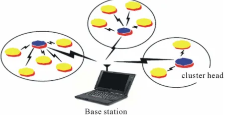
many types of physical parameters. Each sensor node has limited energy and in most applications, replacing energy sources are not possible. So lifetime of sensor nodes is highly dependent on energy stored in their battery. Clus- tering is a designing method that used for management of wireless sensor networks. In this method, the network is divided into several independent collections that these collections called cluster. So each cluster contains a num- ber of sensor nodes and a cluster head node. Member nodes in a cluster send their data to relative cluster head node. Cluster head node aggregates these data and send to the base station. Therefore, clustering in sensor net- works has advantages such as data aggregation support [1], data gathering facilitation [2], organizing a suitable

structure for scalable routing [3], and efficient propaga- tion of data in the network [4].

Data gathering in wireless sensor networks is an im-portant operation in these networks and for this purpose

many methods have been proposed. The LEACH2 _[5]

protocol has been considered as a hierarchical basic method. This method is suitable for monitoring applica- tions. Each node periodically senses the information and sends them. In this algorithm, the clustering method has used for data gathering and aggregation. The cluster and cluster head selected randomly, therefore there is no as- surance to select the exact improved number and uniform distribution of cluster head throughout the network. Many improvements in LEACH protocol have been pre-

sented. LEACH-C3 _{method [6] is an example of these}

improvements. In LEACH-C, the forming of clusters is done using a centralized algorithm by the base station in the starting of each period. Base Station uses the received

2_{Low-energy Adaptive Clustering Hierarchy.} 3_{LEACH-Centralized.}

information from nodes for finding the predetermined number of cluster heads and network configuration within the clusters. This information contains position and en-ergy of nodes. Another improvement to this algorithm is the use of estimation. One of these algorithms is LEACH- CE4 _{[7]. In the proposed technique energy level collected}

from all nodes in two primary periods but not collected in the other periods. Instead, the average energy of initial periods is used. Considering that the energy estimation in this method is not precise, this clustering scheme is not efficient and suitable. There is some proposed clustering methods that ABCP [8] and ABEE [9] and HMM [10,11] are samples of them.

Each sensor node is observer of a physical phenome- non. Also physical phenomenon such as temperature and... continuously change in time. So the information provided by sensor nodes is dependent on each other. Some algorithms that based on not sending of correlated data are considered. The TINA5 _{[12] algorithm is one of}

them. In this algorithm the sensor node compares the value of sampled data with previous data, if that be dif- ferent send it and otherwise goes to sleep mode. The proposed improvement to this algorithm is that sensor node decides to send data with comparing the value of new sample with last reported data [13]. These men- tioned algorithms due to error in report, is not suitable. Therefore, a method proposed to increase the accuracy of data reporting. For precise estimation of nodes energy, the base station must be aware of data time correlation. So with existence of data time correlation and using en- ergy estimation of nodes, a method suggested so that the base station can estimate nodes energy precisely. These methods avoid the overhead excess and increase the net- work lifetime.

The remaining of this article is organized as follows: In Section 2 related works are reviewed. In Section 3 we introduce correlated data algorithm with the energy pre- dicting technique and the hybrid method. Analysis of experiments with existing nodes offered in Section 4, and we finally in Section 5 summarize and discuss the sche- me.

2. Related Work

2.1. LEACH

One of the most famous hierarchical routing protocols based on clustering, is the LEACH protocol. In this method, each cluster members send their data to cluster head. The cluster head aggregate this data and send to the BS. So the communication cost is reduced. Figure 1 de-

scribes this concept:

The operation of cluster forming and data transmission

in LEACH is done in two phases that these phases shown in Figures 2 and 3:

Setup phase is the stage of forming cluster and cluster head. At this stage, cluster and cluster head randomly selected. After forming the cluster, cluster head propa- gate TDMA6 _{scheduler to specify the data transfer time}

to member nodes. Then the steady-state phase started. In the steady-state phase, each member node in cluster send data to the cluster head only in its time slot and at the rest of time pieces for energy conservation goes to sleep mode.

In this method, the cluster head consumes more energy for receiving, processing and directly sending this data to the BS node. So for increasing the life time of the net- work it is necessary to replace role of cluster head be- tween network nodes. Many improvements over the LEACH method have been provided that in these im- provements firstly, as far as possible the best clustering and cluster head selection is done, secondly possible as possible overhead of the protocol is to be reduced. LEACH- C method is an example of these improvements.

2.2. LEACH-C

In LEACH-C, clusters forming in the beginning of every period are done, using the centralized algorithm by the base station. The base station uses received information from nodes that includes energy and node status, uses

Figure 1. A sensor network with clustering.

Figure 2. Period of LEACH.

Figure 3. Details of period. 4_{LEACH-C-Estimate.}

this information during the setup phase for finding pre- determined number of cluster heads and network con- figuration within the clusters. Next classification of nodes in the clusters is done to minimize energy consumption in order to transfer their data to the related cluster head. Results show that LEACH-C overall performance is bet-ter than LEACH because of the optimal forming of clus-ters by the base station. In addition, the number of cluster heads in each period of LEACH-C is equal to the ex-pected optimal value. While in LEACH the number of cluster heads varies in different periods because of lack of global coordination.

As in LEACH-C at the beginning of every period en- ergy of nodes must be sent to BS, therefore nodes early discharged and the network lifetime reduces. Another improvement on this algorithm is the use of energy esti- mation. The LEACH-CE method is an example of these methods.

2.3. LEACH-CE

In the LEACH-CE method, the energy level of all nodes collected only in two primary periods and not be col- lected in other periods. Instead because of knowing in- formation about energy level of nodes, we can calculate energy consumption average for each node by using in- formation of two primary periods. This means that re- ducing calculated energy level from the energy level of node, causes predicting current energy level of node. The problem of this algorithm is that firstly energy estimation is not done precisely and secondly if nodes have corre- lated data, while not sending correlated data means that previous data is valid, so this plan of clustering is not suitable and efficient.

2.4. TINA

Phenomenon that observed by sensor nodes, continu- ally change in time. Therefore information received by the nodes is correlated on each other. These cases for physi-cal phenomena that are continuous or repetitive, or in an application that the accuracy is not too important, or in a network that node density in a region is high, have seen more. There are two types of data correlation: 1) spatial correlation; 2) Time correlation.

In the spatial correlation, aggregation is done within the network by cluster heads. This is one of the proposed methods to reduce energy consumption. So the nodes that have correlated data send them to cluster head and cluster head after aggregating these data send to the base station. This causes to prevent waste of energy. This method has been implemented in LEACH protocol.

But in the time correlation, each node can have corre- lated data in successive times. Mohamed and Sharaf proposed the TINA algorithm. The main idea of TINA

algorithm was that the sensor nodes send their data only when this data differ with previous data otherwise goes to sleep mode. This algorithm has a reporting error. There is an improvement to this algorithm that presented below.

2.5. Improvement of TINA

In this method, the sensor node decides to send data by comparing the value of newly sampled data with last reported data. However, sensor nodes maintain last re- ported data. For better understanding, we describe this section with an example. Suppose that a given sensor node that received data are 1.0, 0.95, 1.05, 0.95, 1.05 respectively. A threshold has been considered that data changing to this threshold is not important. The value of this threshold considered equal to 10%. First given data that is equal to 1.0 successfully sent and in the next pe-

0.95 1.0

5% 10% 1.0



 

riod 0.95, will not be sent when:

Otherwise that will be sent. In the third stage 1.05 1

5% 10% 1



  that will not sent and in the fourth

stage 0.95 1 5% 10%

1 

  that will not sent. This me-

thod is suitable when phenomenon changes have not a lot of swing or any special event in the network is done. But as mentioned previously most of phenomenon change continuously with time. So most of data are in ascending or descending mode in the time slices. Or in an applica- tion such as temperature for example in a certain time slot occurs a specific event. So the proposed methods have errors and are not suitable. We offer a method to improve this algorithm and prevent the waste of energy. In addition, the problem of data time correlation is not considered in proposed protocols. Therefore, we will check the time correlation of data in the proposed algo- rithms.

3. The Proposed Method

3.1. Presentation of Methods

Three ideas are proposed here: 1) the data time corre- lation; 2) Energy estimation model of nodes and 3) the hybrid method.

In the data time correlation algorithm, Time Series Forecasting method (TSF7_{) used to decide sending or not}

sending of data. Then in time t in the beginning of each period, base station send percentage of error e(t) to all nodes. First data sensed by node and sent. Second and third and fourth data sent based on the improved TINA algorithm. Then the node runs time series function to

determine the value of prediction of trend line model, to create trend model. In the next times the sensed data compared with predicted value of trend model, if the difference between these two values exceeds a threshold value, data sent to the given node and the node recalcu- late prediction function of trend model to update the trend line. Otherwise, the sensor node does not send the sensed data with this insurance that sensed data placed in accuracy range of data. So only some data have to be sent that are very different from the trend line model. This help to prevent energy loss.

We call the node energy prediction model LEACH- CEC8 _{and describe as follow. For doing the best cluster-}

ing, that is needed to know energy of the nodes. The es- timation method is a method that has low cost and is suitable. We also use the energy estimation method. For this, we divided LEACH-C protocol to three phases. To-pology building phase, setup-state and steady-state. In the first phase nodes send their position to the BS. Then BS creates network topology based on these positions. Once the topology was formed in the base station, base station node calculates the distance of nodes to each other. The BS calculates the amount of energy used in each node in the setup-phase, using a simple mathemati-cal model. Then deduct this amount from primary energy and calculates its remaining energy. Finally do the clus-tering and goes to the steady-state phase. In this phase for each node, the data time correlated algorithm applied according to the following method.

BS node should be informed of data time correlation in nodes to estimate precisely energy of them. Therefore cluster head create a table that containing list of all members of the cluster. Cluster head registers every node in to the table that have correlated data and do not sent in certain times. In the end of each period, cluster head sends this table with collected data to the base station. This table contains nodes ID and number of times that these nodes not sent data. Base station uses this informa- tion for clustering decisions in centralized methods. Ul- timately that cause to energy estimation in centralized methods is more carefully while the best clustering is created and the network lifetime increases. So in total lifetime of the network, first phase has done once but setup and steady-state phases done as in LEACH-C.

3.2. Process of Proposed Methods

3.2.1. Linear Prediction Method Using Time Series

Linear prediction method is a powerful technique to pre- dict time series in an environment changing with time. Suppose that you want to contact an independent variable

x and a dependent variable y to specify. If we assume that the true relationship between these variables in a straight

line and the value observed for each value of y for every given x is a random variable then we can wrote:

 

E y x a a x (1)

where in this equation a0 is the width from the origin

and a₁ is the slope of the line that is unidentified fixed values. Observed value y can be described with the fol- lowing equation where the error ε created because of not conforming real value to the amount of predicted value.

0 1

y a a x (2)

This pattern is usually named a simple linear regres- sion model. Because that has only one independent vari- able so that the x independent variables called prediction variable and y called the response variable. Prediction and response variables x and y can be time series in which case we have a time series regression pattern.

There are several methods to estimate unknown pa- rameters a₀, a₁ in Equation (2) that can be used. One method that a lot used is the least square error method in which the a0, a1 estimates obtained from minimizing

sum of squares errors or remaining’s. Suppose we have n observations of (x1, y1), (x2, y2) ··· (xn, yn). A model that is based on these observations is written as follows:

0 1 , 1, 2, ,

i i i

y a a x  i  n (3) And the total square error is as the follow:









0 1 0 1

1

, n i

i

a a y a a x









So the total square error is simply the total squares of deviations observed yi and a0a x1 i. The estimated val- ues of a0 and a1 that we call them a0 and a1 that

achieved using the least squares method by minimizing





 toward a₀ and so we can write: a₁





1 0

2 n i i 0

i

y a a x

a        







1 1

2 n i i i 0

i

x y a a x

a        



This system of equations called least squares line normal equations system that simplified as the following:

0 1

1 1

n n

i i

i i

na a x y

 







2

0 1

1 1 1

n n n

i i

i i i

a x a x x y

  

 







By solving this system a0 and a1 estimates or on

the other hand and obtained and so:

8_{LEACH-CE-Correlation.}

0











1 1 1

1 2 2 1 1 1 2 1 ˆ

n n n

i i i i

i i i

n n i i i i n i i xy i n xx i i

x y x y n

a

x x n

x x y y _s

s x x             _  _{ } _     _ _     















a  y a x

where 1 1 n i i x x n 





1 1 n i i y y n 





linear regression model is as follows:

0 1

ˆ ˆ

y a a x

For each value of the predicted variable x we can ob- tain corresponding value predicted response from this equation. The fitted values of yˆ_i corresponding to ob- served values xˆ_i for every i = 1, 2, ···, n is the follow- ing:

0 1

ˆ ˆ

i i

y  a a x

The difference between ith given fitted value to an observed yi value called a residue so that:

ˆ_{i i} ˆ , 1, 2, ,_i

e  y y i  n (5) If the fitted model regression for data is appropriate, in this case remains do not follow of appropriate form. There is no clear pattern for the remains.

This method stated by Equation (11) that is a recursive method [9]:

Linear prediction method is a powerful technique for predicting time series in a time-varying environment. This method is expressed in Equation (6) and is a recur- sive method [9,10]:





 













y t T a y t a y t T   a y t m T (6) Estimated value at time t as a linear function of previ- ous values in the times “t − T, t − 2T, ···, t − mT” has been produced is obtained. In Equation (1) a1, a2, ···, am are the linear prediction coefficients, “m” is the model degree, “T” is the sampling time, y(t + T) is the next ob-servation estimation and y(t), y(t − T),…, y(t −mT) are the present and past observations. The prediction error which is the difference between the predicted and the real values (Equation (7)) must be minimized.

 

Error % *100%

Real value       

 (7)

In order to estimate the coefficients of linear predic-tion model we use the least squares error method and

rewrite Equation (6) with considering modeling error in Equation (8):

 











  

1 2 2

m

y t a y t T a y t T a y t mT e t

   

    (8)

The error e(t) is generated because of not adopting the linear prediction model to the real value. So to find the coefficients, a1, a2, ···, am in Equation (8) we use the sum least squares error and set of linear functions. Presented in Equation (9).

 









  



































 









y t y t T y t mT y t

y t T y t m T y t T

y t mT y t k T y t m k T a e t

a e t T

a e t kT

         _  _{  }    _{ }                              _     _{ }       _               (9) Y    A E (10) Elements in the matrix A are the coefficients which can be found by least squares error method (11):

 

A    Y (11) In Equation (11), φT_{, is the transpose of the matrix φ,} and (φT_{φ) is the inverse of matrix. In practice:}

 If m is chosen larger than is required (i.e. over-estima- tion of the model order), Equation (11), cannot be solved for any unique set of coefficients, because of some columns in the matrix φ, are not independent of each other. Hence φT_{φ would be unique and will not} have inverse. This means that the system of equations in Equation (8) will have an infinite number of an-swers for the coefficients. Geometrically speaking, it is like fitting an infinite number of lines to a single point which is not the preferred case.

 If m is chosen less than the required value, the number of independent equations would be more than the number of unknown variables (a1 – am). Such a sys-tem of equations has to be solved for the best ap-proximation of coefficients. The best apap-proximation for coefficients (a1 – am) is the use of the least squares error method.

Obviously, that is how much precision, the number of the data sent will increase and vice versa.

3.2.2. The Algorithm Used to Estimate the Energy by Transferring Topology to the Base Station

three phases: topology building phase, setup-state and steady-state and this algorithm is proposed as following. These three phases is called LEACH-CEC.

a) Topology building phase

1) Start of network.

2) Base station receives position of all nodes that con-tain x and y.

3) Base station calculates distance of all nodes with each other’s using the following Formula (12):



 



ab a b a b

d  x x  y y 2 (12)

4) End of phase.

b) Setup-state phase

5) If clustering has changed

5.1) BS calculate energy consumption per node using the Formulae (13) and (14):

 

:

elec friss amp crossover

Tx

elec two ray amp crossover

lE l d d d E l d

lE l d d d

            

 (13)

and

 

E l lE_elec (14) And after computing, place the sum of two variables in to the _Et .

ni

5.2) Base station calculates remaining energy (ER) of each node using the Formula (15).

t

R R

E E E_ni (15) 5.3) BS audit the information received from CHs, if the nodes name with the number of duplicate data is there, considered in terms of computing nodes remaining energy.

5.4) If E_R0 the node is dead.

5.5) Otherwise the node is alive and participates in Clustering.

6) Clustering is formed. t

ni: The amount of consumed energy by node i in

E time t.

c) Steady-state phase(Hybrid method)

7) If node n is a cluster head.

7.1) Cluster head creates a table containing node name and the number of correlated data.

7.2) Cluster head collects data from the members of the cluster.

7.3) If the cluster head has not received data from its member node, registers name of that node in the table and a unit to be added to the number of correlated data. Cluster head sends the table with correlated data to the base station.

8) Otherwise, that is a member node.

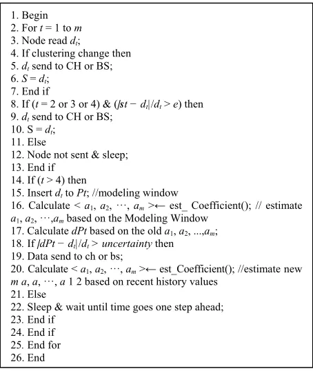
8.1) If the node is in turn on then the node runs corre- lated data algorithm in Figure 4.

8.2) Otherwise goes to sleep mode.

1. Begin 2. For t = 1 to m

3. Node read dt;

4. If clustering change then 5. dt send to CH or BS;

6. S = dt;

7. End if

8. If (t = 2 or 3 or 4) & (|st − dt|/dt> e) then

9. dt send to CH or BS;

10. S = dt;

11. Else

12. Node not sent & sleep; 13. End if

14. If (t > 4) then

15. Insert dtto Pt; //modeling window

16. Calculate < a1, a2, ···, am>← est_ Coefficient(); // estimate a1, a2, ···,ambased on the Modeling Window

17. Calculate dPt based on the old a1, a2, ...,am;

18. If |dPt − dt|/dt > uncertainty then

19.Data send to ch or bs;

20. Calculate < a1, a2, ···, am>← est_Coefficient(); //estimate new m a, a, ···, a 1 2 based on recent history values

21. Else

22. Sleep & wait until time goes one step ahead; 23. End if

24. End if 25. End for 26. End

Figure 4. Algorithm of not sending correlated data using TSF.

 

TX amp : Strengthening the energy to transfer-

E l d

ring 1 bit data in distance d. friss amp

  : Radio energy of amplifier.

two ray amp

   : Radio energy of amplifier.

d: distance between receiver and sender

l: length of data package.

Table 1 should be created by the cluster head in the

steady-state phase. To explain this part, consider a cluster with node numbers 2, 3, 5, 6, 7, 14, and 15 are chosen. Assume that the node 7 is cluster head and the rest is member nodes. If nodes 2 and 5 respectively, each have 2 and 1 correlated data, node 7 as cluster head must cre- ate Table 1. This table must be dynamic and at the end

of each period must be sent with correlated data.

4. Simulation and Evaluation of Methods

4.1. Simulation Environment

Simulations have been done on the Redhat9.0 Linux operating system by using NS2 network simulator. LEACH and LEACH-C protocols Implementation are from the Uamp project at MIT University on NS2.

Table 1. Information of node’s correlated data in BS.

Number of data correlated Node name

2 Node2

1 Node5

center of the network and the latter is in position (50 and 100), which is near the area under monitoring. Each period of simulation takes 20 seconds long. Receivers and transmitters follow the model that their parameters are:

8

5.0 10 J bit , 5.0 10 J bit

elec tx rx

E _{ }  E _E _{ } 8

11 2

-

-15 4

-

-1.0 10 J bit/m , 1.3 10 J bit/m free space amp

two ray amp

 





 

 

,

tx rx

E E are Send and receive power needed for each

bit. Simulations have done using LEACH, LEACH-C, LEACH-CE and LEACH-CEC protocols.

Simulation assumptions:

1) All nodes are static and have limited resources. 2) Base station has not limited resources.

3) All nodes at any moment have data to send.

4) All Nodes equipped with the location determination

4.2. The Result of Simulation

In the NS2 simulator and also LEACH and LEACH-C protocols, data produced with the Uniform distribution. But in fact phenomenon that seen by sensor nodes are continuously changing with time. Therefore, the infor- mation received by the sensor nodes is correlated. There- fore generated data by the simulator must have a normal distribution.

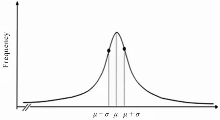
Normal distribution Definition: we say a random va- riable x is normally distributed if its density is as follows:

 





; , e 2

2π

x

x x

f x f x     

 

  (16)

where the parameters μ and σ are     and σ > 0. Each distribution with the given density functions as defined in relation (16), called a normal distribution. To show the parameters we have used μ and σ2 _symbols

because we have known that these are the mean and variance parameters of distribution respectively. Figure 5 shows this concept.

For producing data by normal distribution we assume μ = 0.8 and σ = 1. In the mentioned protocols data generated in uniform distribution. So we have changed the code of these protocols to normal distribution. In addition, the actual amounts of energy in each node in all protocols of LEACH, LEACH-C, LEACH-CE and

LEACH-CEC in each period was calculated. In our first scenario where the base station along the network are located at the point (50 and 100).

Before reviewing mentioned protocols we first survey the data correlation protocols. We will examine TINA, improvement of TINA Protocols and the idea proposed in conjunction with data correlation (TSF). The produced Data by a node in the algorithms TINA, improvement of TINA and the proposed method (TSF) is reviewed. We took this result that the number of data submissions in TSF method is less than previous methods and the accuracy is high. Figure 6 shows this concept.

We have run each of desired protocols 20 times, so that resulting graphs are the average of results of the runs.

Then we calculated the mean of results and by running data correlation algorithms on them we extracted the following results. We concluded that the number of sent data in TSF method is less than two other methods and have a high accuracy. Error Percentage for correlated data in TSF method is equal to 1%.

Diagram of Figure 6 describes this concept. In a pe-

riod in specified times we have generated 20 times ran- dom data and we repeat it again 20 times. Then we cal- culated the average of them and have run the data corre- lation algorithms over them and extracted the following

Figure 5. Data generation model in a node.

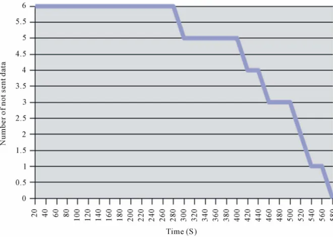
results. of existing correlated data will decrease. In Figure 6 the average of correlated data number in

each period with 100 nodes has shown. Until the 300th time in each moment of sending periods at least 6 data are correlated. From 300th to 400th time there is at least 5 correlated data.

4.3. The First Scenario

In our first scenario where the base station in points (50

and 100) is the network decided Figure 8 shows the

amount of energy consumption in each period. In Figure

8, we compared LEACH, LEACH-C, LEACH-CE and

the proposed LEACH-CEC protocols and then we have considered the value of correlated data in discussed algo- As is clear in the Figure 7 the number of correlated

data throws down over time. Because of nodes energy level decrease over time and then die. So the probability

Figure 7. Average number of correlated data in each period.

Figure 8. Total energy consumption in the network topology.

rithms. Then we have obtained the energy consumptions Value for each of protocols. We called them regularly LEACH-TSF, LEACH-C-TSF, LEACH-CE-TSF and LEACH-CEC-TSF. Finally we compared them with each other. We can see the LEACH-CEC-TSF method has better performance than all of mentioned methods.

Figure 9 shows the number of alive nodes at different

times. In this Figure 9, 8 methods that mentioned above

are assessed by the number of alive nodes in each period.

As in Figure 9, in the LEACH-CEC-TSF method the

number of alive nodes is more than all other methods. In

Figure 9, in the centralized protocols nodes death time

has been started from 400, but in the distributed proto-

cols death of nodes has started from 220.

4.4. The Second Scenario

In the second scenario the base station’s location changed to the point (50, 50). Figure 10 shows energy

consumption in each period. In this scenario first energy estimation of LEACH-CEC protocol has been compared with the LEACH and LEACH-C and LEACH-CE proto- cols.

Simulations show that since the base station is located in the center of the network, so the energy consumption is lower in comparison with the first scenario.

Figure 9. Number of alive nodes in each period.

Figure 11 shows data correlation in each of the

LEACH and LEACH-C and LEACH-CE and LEACH- CEC protocols. Simulations show that data correlation is not dependent on the particular scenario.

Number of live nodes in each of the LEACH, LEACH-C, LEACH-CE and LEACH-CEC protocols without data correlation is compared in Figure 12.

Applying Data correlation to the each of LEACH, LEACH-C, LEACH-CE and LEACH-CEC protocols shows

that live nodes number is further when the base station is located in the center of the network. This operation has shown in Figure 13.

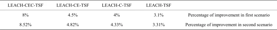
As seen in the distributed protocol, death of nodes started in time 220. But in LEACH, LEACH-C, LEACH- CE and LEACH-CEC centralized protocols death of nodes started in time 360. As seen the proposed methods have better performance than the previously proposed technique presented. Table 2 shows the percentage of

Figure 11. Comparison of energy consumption values by applying data correlation.

Figure 13. Number of live nodes by applying data correlation.

Table 2. Percentage of energy improvement protocols.

LEACH-TSF LEACH-C-TSF

LEACH-CE-TSF LEACH-CEC-TSF

Percentage of improvement in first scenario 3.1%

4% 4.5%

8%

Percentage of improvement in second scenario 3.31%

4.33% 4.82%

8.52%

energy improvement by applying TSF to each protocol.

5. Conclusions

This article solves the problem of correlated data in all of discussed protocols in this paper. So the nodes that have time correlated data and sending this data wastes their energy and thus network lifetime will decrease. By using the algorithm of data time correlation, the problem will be raised. Also we have eliminated periodic sending of nodes data in LEACH-C protocol. By using energy esti-mation in LEACH-CEC method there is no need for nodes to send their energy level and position to the base station. They only have to send their position at the be-ginning of network to the base station and the base sta-tion creates network topology and using a simple mathe-matical calculation will calculate the energy of nodes.

Totally we improved the lifetime of network by using simulation in LEACH, LEACH-C, LEACH-CE and pro- posed LEACH-CEC protocols. Also we improved energy consumption by using estimation methods. In the future works we will try to use classification of nodes distances scheme to estimate energy of nodes more precisely.

REFERENCES

[1] S. Bandyopadhyay and E. Coyle, “An Energy Efficient Hierarchical Clustering Algorithm for Wireless Sensor

Networks,” Proceedings of IEEE INFOCOM, San Fran-cisco, 30 March 2003.

[2] M. Ali and S. K. Ravula, “Real-Time Support and Energy Efficiency in Wireless Sensor Networks,” School of In- formation Science, Computer and Electrical Engineering Halmstad University, Halmstad, 2008.

[3] A. A. Abbasi and M. Younis, “A Survey on Clustering Algorithms for Wireless Sensor Networks,” Elsevier B.V, Amsterdam, 2007.

[4] M. Demirbas and H. Ferhatosmanoglu, “Peer-to-Peer Spatial Queries in Sensor Networks,” Proceeding of 3rd IEEE International Conference on Peer-to-Peer Computing (p2p ’03), Linköpings, 11 August 2003, pp. 32-39. [5] W. B. Heinzelman, A. P. Chandrakasan and H. Balakrish-

nan, “An Application-Specific Protocol Architecture for Wireless Microsensor Networks,” IEEE, Vol. 1, No. 4, 2002, pp. 660-670.

[6] S. D. Muruganathan and D. C. F. Ma, “A Centralized Energy-Efficient Routing Protocol for Wireless Sensor Networks,” IEEE, Vol. 43, No. 3, 2005, pp. 8-13.

[7] W. B. Heinzelman, A. P. Chandrakasan and H. Balakrish- nan, “Application-Speci_c Protocol Architectures for Wire- less Networks,” IEEE Transactions on Wireless Commu-nications, Vol. 1, No. 4, 2002, pp. 1-154.

doi:10.1109/TWC.2002.804190

[8] X. Wang, J.-J. Ma, S. Wang and D.-W. Bi, “Time Series Forecasting for Energy-Efficient Organization of Wire-less Sensor Networks,” MDPI, 2011.

[9] W.-P. Chen, J. C. Hou and L. Sha, “Dynamic Clustering for Acoustic Target Tracking in Wireless Sensor Net-works,” Proceedings of the 11th IEEE International Con- ference on Network Protocols, Atlanta, 4-7 November 2003, pp. 284-294. doi:10.1109/ICNP.2003.1249778 [10] C.-K. Liang, Y.-J. Huang and J.-D. Lin, “An Energy

Effi-cient Routing Scheme in Wireless Sensor Networks,” 22nd International Conference on Advanced Information Networking and Applications, IEEE, Singapore, 22-25 March 2008.

[11] P. Hu, Z. Zhou, Q. Liu and F. M. Li, “The HMM-Based Modeling for the Energy Level Prediction in Wireless

Sensor Networks,” Proceeding of the 2007 2nd IEEE Conference on Industrial Electronics and Applications, Harbin, 23-25 May 2007.

[12] A. S. Mohamed and B. Jonathen, “TINA: A Scheme for Temporal Coherency-Aware In-Network Aggregation,” Proceedings of the 3rd ACM International Workshop on Data Engineering for Wireless and Mobile Access, San Diego, 19 September 2003, pp. 69-76.