Algorithms for Integer Factorization Based on Counting Solutions of Various Modular Equations

Algorithms for Integer Factorization Based on Counting

Solutions of Various Modular Equations

Boris S. Verkhovsky

Computer Science Department, New Jersey Institute of Technology, Newark, USA E-mail: [email protected]

Received September 20, 2011; revised October 27, 2011; accepted November 6, 2011

Abstract

This paper is a logical continuation of my recently-published paper. Security of modern communication based on RSA cryptographic protocols and their analogues is as crypto-immune as integer factorization (iFac)

is difficult. In this paper are considered enhanced algorithms for the iFac that are faster than the algorithm

proposed in the previous paper. Among these enhanced algorithms is the one that is based on the ability to count the number of integer solutions on quadratic and bi-quadratic modular equations. Therefore, the iFac

complexity is at most as difficult as the problem of counting. Properties of various modular equations are provided and confirmed in numerous computer experiments. These properties are instrumental in the pro-posed factorization algorithms, which are numerically illustrated in several examples.

Keywords: RSA Cryptography, Integer Factorization, Modular Quadratic Equations, Modular Bi-Quadratic

Equation, Equivalent Problems, Rabin Protocol

1. Introduction and Problem Statement

Security of modern communication based on RSA or Rabin cryptographic protocols and their analogues is as crypto-immune as difficult is the integer factorization (iFac) [1-3]. This paper is a continuation of the paper [4]. In that paper is considered a factorization algorithm of semi-prime n=pq for two cases: where either both factors p and q are non-Blum primes i.e.,

p=q=1(mod4), (1.1) or at least one factor is a non-Blum prime. In this paper an iFac algorithm is provided, which also works if both factors p and q are Blum primes, i.e.,

p=q=3(mod4). (1.2) The SQUAR-algorithm discussed in [4] is based on several properties (formulated as propositions and con-jectures) of dual modular elliptic curves, where b is a positive integer:







2 2 2 _mod

y x x b n





; (1.3)

and 2



2 2





_mod . (1.4)

y x x b n

Let us reiterate some of these properties and then con-sider their generalizations.

Let p=q=1(mod4); n=pq; let P(n,b) and M(n,b) denote the number of points on elliptic curves (EC) (1.3) and (1.4) respectively.

For the sake of brevity, we call P(n,b) and M(n,b) the counts.

Conjecture 1.1: Consider n=pq, and let primes p and q satisfy (1.1);

if P n

 

,1 M n



,1



; (1.5) then for every integer b

 

,



P n b M n b,



; (1.6) otherwise, for every integer b

 

,



P n b M n b,



. (1.7) If n is a prime and (1.5) holds, then for every b also holds

 

,

 

, 2 P n b M n b n

  . (1.8)

Remark 1.1: Conjecture1.1 plays an important role in the design of the iFac described in [4]; further details are provided in the Appendix.

B. VERKHOVSKY 676

if

mod 4 2



m s 



s

2



; (1.9)

then



, 2m





, 2

P n M n . (1.10)

Proposition 1.3: If the factors p and q are congruent to 1 modulo n=pq, b₁b , and



, 1





, 2

P n b M n b ,

then



, 1





, 2



M n b P n b . (1.11)

The proposed iFac2 algorithm described below is less restrictive than the integer factorization SQUAR-algo- rithm described and analyzed in [4], because it is also applicable if both p and q satisfy (1.1).

Proposition 1.4: {modular reduction-in-exponent}: Consider elliptic curves







2 2 e _mod y x x b n





; (1.12)

and







2 2 e _mod

y x x b n ; (1.13)

where ; then for every integer b>0 and e>0 the following identities hold:

4 e

  

_, e _, emod 4



P n b P n b ; (1.14)

 

_, e _



_, emod 4



M n b M n b . (1.15)

Proof {by mathematical induction}: Consider substitu-tions

3

: mod and : 2mod

y Yb n xXb n; (1.16) into (1.12). Then after cancellation of the same term in both parts of (1.12) we derive the EC

6

b







2 2 e 4 _mod

Y X X b n









. (1.17)

Repeating the substitutions (1.16) and cancellations of term , we derive the proof of (1.14). Analogously we proceed with the proof of (1.15).

6

b

A generalized reduction-in-exponent can be formulated for a hyperelliptic curve {HEC}.

Proposition 1.5: Consider HECs



t





mod

r d e

y  x x b n ; (1.18)

and r



d t emodd t r m/



_mod . (1.19) Y  X X b    n

If t<d and gcd(d, r)=m, then for every integer b>0 both HECs have equal number of points.

Proof: after appropriate substitutions, the proof is analo-gous to the proof of Proposition 1.4 (details of the proof

and an example are provided in the Appendix}. Special case: if m=1 and t=0, then



mod





_mod

 

r d e dr

Y X b n



. (1.20)

2. iFac1 Algorithm Based on EC

SQUAR-algorithm described in paper [4] requires con-sideration of a sequence of elliptic curves with control parameter b. Namely, for every b=1,2,3,5,··· to count the number of points on each EC until four distinct counts are found; {see Example 2.1 below}.

In the following algorithm we need at most three distinct counts. Let P_i:P n b



, _i



.

The iFac1 algorithm:

1) Compute P P1, , ,2 PiP1 until two distinct integers are found;

2) if sign P



1n



sign P



in



(2.1) then p: gcd



P1P ni, ;



q=n/p; (2.2)

else compute w: gcd



P1Pi,n



; (2.3) 3) if w>1, then p:=w; (2.4) else find a 3rd _{distinct count ;}

k P

4) p: gcd



P1Pk, ;n



q=n/p. (2.5)

Example 2.1: For semi-prime n=6525401, the sets are as follows:

1, , 2 3and 4

S S S S













1 2 3

1,7,11,17, 29,31, 41, ; 7012681 ; 2,5,13, 23,37, ; 6055665 ; 3,19, ; 6514053 ;

S b L

S b S

S b A

            (2.6)

S4={b=43,53,···; B=6519205}.

Therefore, the SQUAR-algorithm provided in [4] re-quires at least fifteen basic steps, because 43 is the four-teenth prime (2.5). Yet, since

1

P P₂; andP₁P₃P₂; (2.7)

then the 1st





1 3

: gcd , factor  PP n . Hence, instead of counting points

1, , , , , ,2 3 5 7 43

P P P P P  P [4], in fifteen elliptic curves, we determine both factors of n after three distinct counts.

3. iFac1 Validation

Definition 3.1: A pair of counts is called a

resolventa if



, i j P P







gcd PiP nj, 1.





Proposition 3.1: If primes p and q are selected ran-domly, then with probability greater than 2/3 we can determine factors of semi-prime n if we know only two distinct counts ₁ and . i

Proof: It is demonstrated in the paper [4] that if p=q=1(mod4), then there exist two positive integers c<p and d<q, and four sets 1 2 3 4 such that for every b the number of points on the elliptic curves (1.3) and (1.4) is equal either A or B or L or S, where

P P

, , and

S S S S









: ;

: ;

A p c q d

B p c q d

  

   (3.1)











: ;

: ;

L p c q d S p c q d

  

  



(3.2)

{see Example2.1}.

For instance, let’s analyze

gcd(L+S, n); (3.3) where L+S=2(n+cd) (3.2). (3.4) Let’s find under what conditions p divides L+S: suppose that

n+cd=ph, (3.5) where h is an integer. Then (3.5) implies

that (n+cd)modp=phmodp=0; (3.6) and cdmodp=0. (3.7) Since c<p, therefore, p must divide d.

Hence, if c  p d q, and p|d, (3.8) then we can find factors p and q after considerations of only two distinct counts ₁ and _i. Although this case is possible {see Example 3.2}, for large primes p and q it is highly improbable.

P P

Analogously, we proceed with an analysis of gcd(A+B, n). Example 3.1: Consider n=9037729;

and EC _y2 _x3_x



_modn



_{. (3.9)} If P1A=8894593; Pi B=9176905; then compute

w:=gcd(A+B, n)=1.

Since w=1, it means that we cannot find the factors of n because the combination {A, B} is not a resolventa {see Table 3.1}. Yet, after we find the third distinct value

=L=9342205; the factorization is accomplished: k

P

p=3361 and q=2689.

Example 3.2: {Highly improbable case}: Consider n=24853. Let’s verify that, if we know any two counts, we can find p and q. There are six cases to consider: 1). P₁=A; P_i=B; 2). =A; P₁ P_i=L;

3). P₁=A; P_i=S; 4). =B; P₁ P_i=L;

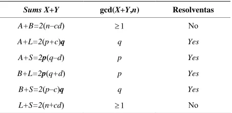
[image:3.595.311.538.94.205.2]

5). P₁=B; P_i=S; 6). =L; P₁ P_i=S;

Table 3.1. Sums and greatest common divisors.

Sums X+Y gcd(X+Y,n) Resolventas

A+B=2(n–cd) 1 No

A+L=2(p+c)q q Yes A+S=2p(q–d) p Yes B+L=2p(q+d) p Yes

B+S=2(p–c)q q Yes L+S=2(n+cd) 1 No

where A=17385; B=31161; L=35685; and S=15181. Then for each of these combinations we find a factor of n. In-deed,

gcd(A+B,n)=29; gcd(B+L,n)=857; gcd(B+S,n)=29; gcd(A+L,n)=29; gcd(A+S,n)=857; gcd(L+S,n)=29.

Although such case is possible, it is highly improbable if p and q are randomly selected.

Example 3.3: Consider n=8405801 and EC (3.9). Compute ₁=8387409; = ; =8995597; and w:=gcd( + , n)=2801.

P P

2

P P₁ P₃

1 3

Because w>1, therefore P

p:=w and q:=n/p=3001.

In general, every combination {A, L}, or {A, S}, or {B, L} or {B, S} has a common factor. Hence, if w=1,

then gcd



P1P nk,



1, (3.10) otherwise gcd



P₁P ni,



1. (3.11) Since n is a semi-prime, then in each of these cases we compute a factor of n. For instance, if

1= and i P A PL,

then A L



pc q



; (3.12) and gcd_



pc q n



, _q. (3.13) For more details see Table A2.

Although the iFac1 algorithm is computationally simpler than the SQUAR algorithm, we can further simplify the iFac algorithm via application of other modular equations.

4. Modular Quadratic and Bi-quadratic

Equations

In this section are considered properties of quadratic, bi-quadratic modular equations and equations with , where the moduli are prime or semi-prime.

3 m

Proposition 4.1: Consider a modular quadratic equa-tion (MQE)



2_ 2_{ mod}

B. VERKHOVSKY 678

let G(n, b) denote the number of integer pairs (x, y) {called points on quadratic curve (4.1)} that satisfy (4.1); if n is a prime, then for every non-zero b co-prime with n

 

, 1 G n b  n ;

if n is a semi-prime and n=pq, then for every non-zero b co-prime with n



,

 

1





G pq b  p q1 . (4.2) Proof is provided in the Appendix.

Conjecture 4.2: Consider a modular equation V(p, m, b):





2 2m _mod

y x b p ; (4.3)

where p is a prime; let G(p, m, b) denote the number of points on (4.3);

if (4.3) is either a quadratic or bi-quadratic equation (i.e., if m=1 or m=2), and pmod4=3, then



, ,



 1.

G p m b p (4.4) if m=1 and pmod4=1, then (4.4) holds.

Table 4.1. Values of G(p, m, b).

pmod4 m=1 m=2 m≥ 3: if gcd(m,p–1)=1 pmod4=1 p1  p 1 p1

pmod4=3 p1 p1 p1

Conjecture 4.3: Consider a modular equation V(n, m, b): let b>0;



2 2m _mod y x b n







1 ; (4.5)

and let G(n, m, b) denote the number of points on (4.5); if both factors p and q are primes, and if (4.5) is either a quadratic or bi-quadratic equation (i.e., if m=1 or m=2), then for every b>0



, ,

 

1



1

G pq m b  p q ; (4.6) if an odd prime m is co-prime with , then for every b and m each co-prime with





1 p q

 

n 



, ,

 

1



1





[image:4.595.309.537.167.248.2]

G n m b  p q  n



. (4.7) Here 

 

n is called the Euler totient function.

Table 4.2. Values of G(pq, m, b).

m=1 m=2 m>3; if gcd_m, n_=1 p=q(mod4)=1  n  n  n

p=q(mod4)=3  n  n  n pqmod4=3  n  n  n

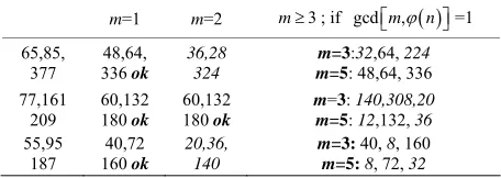
Numerous computer experiments for m=2, 3, 5, 7 con-firmed Conjecture 4.3 Thirty six examples in Table 4.3 demonstrate the correctness of the Conjecture 4.3 for m=1, 2, 3, and 5. In italics are shown the cases, where

 

gcd_m, n _>1, i.e., where (4.7) does not hold.

Table 4.3. Values of G(pq, m, b); m=1,2,3,5.

m=1 m=2 m3; if gcd_m, n_=1 65,85,

377

48,64, 336 ok

36,28 324

m=3:32,64, 224 m=5: 48,64, 336 77,161

209

60,132 180 ok

60,132 180 ok

m=3: 140,308,20 m=5: 12,132, 36 55,95

187

40,72

160 ok 20,36, 140

m=3: 40, 8, 160 m=5: 8, 72, 32 {see also Table 6.1 and 6.2 below}.

The iFac algorithm described below is based on Pro-position 4.1. This algorithm is computationally efficient if there exists an efficient procedure (an oracle) that counts the points on either the MQE (m=1) or bi-quadratic equation (m=2) (4.5).

Definition 4.1: {equivalence}: Problem A1 is equi- valent to problem A2 if their time complexities satisfy the inequality T A

 

1 T A

 

2 .

Definition 4.2: {strong equivalence}: Problems A1 and A2 are strongly equivalent if their time complexi-ties T₁ and T₂ satisfy 

 

T₁  



T₂



1 .

Tables 6.1 and 6.2 illustrate Conjecture 4.2 and Conjec-ture 4.3.

5. iFac2 Algorithm

Conjecture 4.3 can be applied to design an iFac2 algo-rithm. As it implied from the following discussion, this algorithm is more efficient than the SQUAR-algorithm proposed in [4]. Yet, for the seemingly simple iFac2 algorithm we need to know how to efficiently count the number of points G(n, m, b) on modular Equation (4.5) for m=1 or m=2.

The algorithm

1) Select b=m=1; compute G(n) for V(n,1,1) (4.5) and (4.6);

2) Compute

 

:

R  n G n  ; (5.1)

3) Solve quadratic equation

2 ₀

z Rz n ; (5.2) suppose 1 2 are its roots;

4) {Integer factors p and q}: and

z z

2 1

: and :

p z q z . (5.3)

[image:4.595.57.287.630.718.2]

and Remark 5.1: It is well-known that, if n is a semi-prime

and if we know the value of Euler totient function 

 

n (4.7), then we can find the factors of n. The Conjecture 4.3 is the framework that allows us to compute 

 

n .

 

: 1 19874

R  n G n   .

The quadratic equation

2 _{19874 98743069 0}

z  z  ; (5.4) Example 5.1: Let n=98,743,069;

has two roots: then

1,2 9937 30

z   .

[image:5.595.59.542.205.275.2]

G(n)=98,723,196;

Table 6.1. V(p, m, 1): 2 2





= m 1 mod

y x  p .

p m = 2 m = 3 m = 5 m = 7 * p m = 2 m = 3 m = 5 m = 7

59 58 58 58 58 * 2011 2010 2186 2162 2010

101 98 100 92 100 * 2017 1998 2084 2016 2284

1777 1854 1748 1776 1776 * 99923 99992 99992 99992 99992

[image:5.595.57.540.307.366.2]

1913 1998 1912 1912 1912 * 99991 99990 101102 101102 99990

Table 6.2. V(p, m, 1) for 6 7

10  p 10 .

p m = 1 m = 2 m = 3 m = 5 m = 7

2,696,527 2696526 2696526 2689958 2696526 2701694

5,264,647 5264646 5264646 5273726 5264646 5264646

6,878,407 6878406 6878406 6875918 6878406 6878406

Therefore, by the Vieta theorem, p and q are the roots of quadratic equation

Hence,

1 2

: =9967 and : 9907

p z q z  .





2 _{1 ,}

z _n G n m _z n 0. (7.3)

6. Properties of Modular Equations for m>1:

Computer Experiments

Q.E.D

8. Conclusions

Table 6.1 describes results of computer experiments for

various primes p and _{Several factorization algorithms were described and ana-} lyzed in [4] and in this paper {see Table 8.1}. It is obvi-ous that modular Equation (4.5) can be used for the iFac2 only if either m=1 or m=2. From the paper it fol-lows that the complexity of integer factorization is at most as difficult as the problem of counting how many solutions have modular Diophantine equations. There-fore, the problem of counting points on the MQE is equivalent with the iFac2 problem.





2 2m _{1 mod}

y x  p . (6.1)

Remark 6.1: In Tables 6.1 and 6.2 in italic are indi-cated cases where G m p



,



 p 1 if gcd



m p,  1



1. Notice that since





101 1777 1913 2017 1 mod4 ,   

[image:5.595.311.537.609.700.2]

the bi-quadratic modular equations do not have exactly p–1 points.

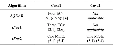
Table 8.1.Algorithms & residues modulo 4.

7. iFac2 Algorithm Validation

Algorithm Case1 Case2

SQUAR _{(8.1)-(8.8); [4]} Four ECs: Not

applicable

iFac1 Three ECs: _(2.1)-(2.6) Not

applicable

iFac2 One MQE: _(5.1)-(5.4) One MQE: _(5.1)-(5.4) From Conjecture 4.3, the number of points G(n,m) on

modular Equation (4.5) is equal



,

 

1



G pq m  p q1 . (7.1)



If there is a computationally efficient algorithm that computes G(n,1) or G(n,2), then it implies that for m2

Case1: p=q=1(mod4) or (p+q)mod4=0;



1 ,

B. VERKHOVSKY 680

9. Acknowledgements

I express my appreciation to A. Joux, D. Kanevsky, A. Koval, R. Rubino and to reviewers for suggestions that improved this paper.

10. References

[1] R. L. Rivest, A. Shamir and L. M. Adleman, “A Method for Obtaining Digital Signature and Public-Key Crypto-systems,” Communications of ACM, Vol. 21, No. 2, 1978, pp. 120-126. doi:10.1145/359340.359342

[2] H. Elkamchouchi, K. Elshenawy and H. Shaban, “Ex-tended RSA Cryptosystem and Digital Signature Schemes in the Domain of Gaussian Integers,” Proceedings of the

8th International Conference onCommunicationSystems,

Singapore City, Vol. 1, 25-28 November 2002, pp. 91-95. [3] M. O. Rabin, “Digitalized Signatures and Public Key Func-

tions as Intractable as Factorization,” Technical Report MIT/LCS/TR-212, MIT Laboratory for Computer Science,

Cambridge, January 1979.

[4] Boris S. Verkhovsky, “Integer Factorization of Semi-

primes Based on Analysis of a Sequence of Modular El-liptic Equations,” International Journal of Communica-tions, Network and System Sciences, Vol. 4, No. 10, 2011,

pp. 609-615. doi:10.4236/ijcns.2011.410073

[5] C. Pomerance, “The Quadratic Sieve Factoring Algorithm,”

Advances in Cryptology, Proceedings of Eurocrypt’84, LNCS, Vol. 209, Springer-Verlag, Berlin, 1985, pp. 169-

182.

[6] R. Schoof, “Counting Points on Elliptic Curves over Fi-nite Fields,” Journal de Theorie des Nombres de Bor-deaux, Vol. 7, No. 1, 1995, pp. 219-254.

doi:10.5802/jtnb.142

[7] K. Rubin and A. Silverberg, “Ranks of Elliptic Curves,”

Bulletin (New Series) of the American Mathematical So-ciety, Vol. 39, No. 4, 2002, pp. 455-474.

[8] L. Dewaghe, “Remarks on the Schoof-Elkies-Atkin Al- gorithm,” Mathematics of Computation, Vol. 67, No. 223, 1998, pp. 1247-1252.

doi:10.1090/S0025-5718-98-00962-4

[9] C. F. Gauss, “Theoria Residuorum Biquadraticorum,” 2nd Edition, Chelsea Publishing Company, New York, 1965, pp. 534-586.

Appendix

A1. Proof of Proposition 4.1

Consider MQE:





2 2 _mod

y x b n . (A.1)

Proposition 4.1: If n is a prime, then the number of points with non-negative x and y on quadratic curve Q(n) is equal n–1; if n=pq, then Q(pq)=(p–1)(q–1).

Proof: Consider an integer parameter t on interval [1, n–1]. The modular multiplicative inverse of t exists if and only if gcd (t, n)=1.

Consider



1





_{1 2 mod}

 



v t t b n  n ; and



1





_{1 2 mod}

 



w t b t  n n . (A.2)

If n is a prime, then there are n–1 integers that are co-prime with n; if n is a semi-prime and n=pq, then there are (p–1)(q–1) integers that are co-prime with n. If n is odd, then (n1) 2 is an integer; therefore both v and w are integers.

It is easy to verify that for every t there is a unique pair {v, w} that satisfies (A.1). Therefore, we proved that (A.1) has at least n–1 solutions for n prime and has at least (p–1)(q–1) if n=pq. Let us show that there are no other solutions.

Let assume that there exists a solution (g, h) that is dis-tinct from every pair in (A.2). First of all,



2 2 _mod



g h b n



g h



, which implies that, if ,

then neither ;

1  b n 1 modn 0

 

nor



gh



modn0

0

. (A.3) Consider an integer





: mod

u  gh n ; (A.4)

where 1  u n 1; then

1 _mod

g h u b n. (A.5)

Thus,



1



_{2 mod}1

g uu b   n; (A.6)

and



1



_{2 mod}1

h u b u    n. (A.7)

If n is odd, then modular inverse of 2 exists and





1

2 mod n n1 2 modn. (A.8) Hence, the solution (g, h) has the same parametric repre-sentation as (v, w), if u=t. The contradiction proves the

Proposition 4.1. Q.E.D. Example A1: Consider Q(17):





2 2 _{2 mod17}

y x  . There are sixteen points on Q(17):



 

 

 



( 6,0); 0, 7 ; 1, 4 ; 2, 6 ; 7, 8        .

A2. Complexity Analysis

There are several algorithms that count points on elliptic and hyper-elliptic curves. If some of these algorithms can be applied for counting points on quadratic or bi-quad- ratic modular equations with the same time complexities, then the Schoof-Elkies-Atkin (SEA) algorithm is currently the best known algorithm that counts points on a modular cubic curve with expected running time _O



_log4_p



[5-7]. Therefore, if, for instance, p is of order

  

₂1024 ₁₀307



O O , then



_log4

   

₂40 ₁₀12

O p O O



. (A.5) Because the SEA algorithm does not work if a=1 and b=0 [8], consider a modular equation





2 2 2 _mod

y x b p with b 0 and an algorithm with complexity



logs



O p that counts points on this curve. Since there are algorithms with complexity



_log8



O p

8 s

that count points for every elliptic curve, therefore  . Thus



_logs

   

₂10s ₁₀3s



O p O O . (A.6)

This implies that in the worst case the problem can be solved with complexity

 

₁₀24

O .

A3. Proof of Proposition 1.5

Consider hyperelliptic curves (HECs)



t





mod

r d e

y  x x b n



; (A.7) and

 



mod





mod e d t r m t

r d

Y  X X b    n



. (A.8) If 0t<d and gcd(d,r)=m, then for every positive inte- ger b both HECs have equal number of points.

Proof: Consider substitutions : w; : z

xXb y Yb ; (A.9) into Equation (A.7); then we derive



d





mod

r r z dw t tw e

B. VERKHOVSKY 682



 



mod .

rzdw  n (A.10)

The case is simplified if t

 

n and d

 

n . If gcd(r, d)=m; then w=r/m and z=d/m.

Hence, dr rt em i.e. d,



t r m



e.

Therefore, after cancellation of equal terms in both sides of the modular Equation (A.10), we derive a HEC

 







mod

r d t e d t r m

Y  X X b  n



. (A.11) Example A3: Let consider HEC







6 15 11 1777 _mod1913

y  x x b



; (A.12) then HEC 6



15 11





_mod1913

Y  X bX



has the same

[image:8.595.84.512.200.338.2]

number of points as (A.12).

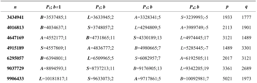
Table A1. # of EC and sequence in which A, B, L and S are computed; here S<A<B<L.

n P1; b=1 P2; b P3; b P4; b p q

3434941 B=3537485;1 L=3633945;2 A=3328341;5 S=3239993;-5 1933 1777

4016813 B=4034637;1 S=3748057;2 L=4294809;5 A=3989749;-5 2113 1901

4647169 A=4552177;1 B=4731865;11 S=4330189;13 L=4974445;17 3121 1489

4915189 S=4557869;1 A=4836777;2 B=4980665;7 L=5285445;-7 1489 3301

6295057 B=6394801;1 L=6509965;5 S=6082957;7 A=6192505;11 2017 3121

9037729 A=8894593;1 S=8737213;11 B=9176905;13 L=9342205;19 3361 2689

9906433 L=10181817;1 S=9633073;2 A=9717861;5 B=10092981;7 5021 1973

Remark A1: In five of seven experiments, the very first two counts {B, L}; {B, S}; {S, A}; {B, L}; and {A, S}

are resolventas, i.e. they provide a factor of n:



1 2

