Parsimonious Support Vector Regression using Orthogonal
Forward Selection with the Generalized Kernel Model
Xunxian Wang†, Sheng Chen‡, David Brown†
† Computer Intelligence & Applications Research Group
Department of Creative Technologies, University of Portsmouth Buckingham Building, Lion Terrace, Portsmouth, PO1 3HE, UK Email: [email protected]
‡ School of Electronics and Computer Science University of Southampton
Highfield, Southampton SO17 1BJ, U.K. E-mail: [email protected]
Abstract
Sparse regression modeling is addressed using a generalized kernel model in which kernel regressor has its individually tuned position (center) vector and diagonal covariance matrix. An orthogonal least squares forward selection procedure is employed to append regressors one by one. After the determination of the model structure, namely the selection certain number of regressors, the model weight parameters are calculated from the Lagrange dual problem of the regression problem with the regularized linear
ε
−
insensitive loss function. Different from the support vector regression, this stage of the procedure involves neither reproducing kernel Hilbert nor Mercer decomposition concepts and thus the difficulties associated with selecting a mapping from the input space to the feature space, needed in the support vector machine methods, can be avoided. Moreover, as the regressors used here are not restricted to be positioned at training input points and each regressor has its own diagonal covariance matrix, sparser representation can be obtained. Experimental results involving one toy example and two data sets demonstrate the effectiveness of the proposed regression modeling approach.Keywords: Regression, support vector machine, orthogonal least squares forward selection, generalized kernel model, sparse modeling
1. Introduction
Having good generalization ability and sparse representation are two key requirements in establishing a learning machine. Forward selection using the orthogonal least squares (OLS) algorithm [1] is a simple and efficient construction method that is capable of producing parsimonious linear-in-the-weights nonlinear models with excellent generalization performance. Alternatively, the state-of-art sparse kernel modeling techniques, such as the relevant vector machine and support vector machine (SVM) [2,3], have been gaining popularity in data modeling applications especially SVM algorithm. Originated from maximum margin linear classification problem, one of the main features of the SVM is to use hyper-plane to do both classification and regression. In classification, the hyper-plane will be adjusted to obtain the maximum classification margin. In regression, the gradient of the hyper-plane will be kept as small as possible. In a SVM type method, the training data are mapped to a high dimensional space where they can be approximated by a hyper-plane. The parameter of the hyper-plane is obtained by minimizing the cost consisted of the linear
ε
−
insensitive loss function and the squared gradient of the hyper-plane. The successfully application of the SVM is heavily depended on the finding of the mapping that is not easy to find unfortunately. And then reproducing kernel Hilbert space theory is used through Mercer theorem.Unlike SVM formulation, the method proposed in this paper minimizes the cost consists of linear
−
standard OLS algorithm [1], in which only the regressor selection procedure is used, here the regerssor parameters will be optimized as well. In fact, at each stage of the selection, the optimization is used with respect to the kernel center vector and diagonal covariance matrix, and the determination of these kernel parameters is performed using a repeated weighted boosting search algorithm [4]. After the selection of a parsimonious model representation, the kernel weights are then calculated from the Lagrange dual of the minimization problem. This proposed generalized kernel regression modelling approach has the potential of improving modelling capacity and producing sparser final models, compared with the standard SVM algorithm. The advantages of the proposed method are illustrated using one toy example.
2. Standard kernel regression modelling
The task of kernel regression modelling is to construct a kernel model from the given training data set , where is the ith training input vector of dimension m, is the desired output with
single dimension for the input and N the number of training data. The SVM method solves the problem by using the following strategy.
N i i i
y
x
,
}
1{
=x
iy
ii
x
2.1 Support vector machine regression problem
In dual space, SVM regression problem can be stated as below:
∑
∑
∑
= + + = − − = − − − = N ji i i j j i j
N
i i i i N
i i i y k x x
L imize 1 , * * 1 * 1 * ) , ( ) )( ( 2 1 ) ( ) (
max ε α α α α α α α α (1)
N i C N i C subject i i N i i , , 1 , 0 , , 1 , 0 0 ) ( to * 1 i * L L = ≤ ≤ = ≤ ≤ = −
∑
= α α α α (2)Where ki,j =k(xi,xj)= ϕ(xi),ϕ(xj) , ϕ(x)is the selected mapping from the input space to a high-dimensional (feature) space, is the regression linear function (hyperplane) in the high
dimensional space, W is the gradient of the hyperplane, C is the regularization parameter.
b x W y= Tϕ( )+
After obtaining αi,αi*,i=1,L,Nand b, the regression model can be given by
b x x k y N i i i
i − +
=
∑
=1 * ) , ( ) (ˆ α α (3)
One of the most common choices of kernel function is the Gaussian function of the form:
⎟⎟ ⎠ ⎞ ⎜ ⎜ ⎝ ⎛ − − = 2 2 2 exp ) , ( σ i i x x x x
k (4)
The common kernel variance is not provided by the algorithm and has to be determined by other means, such as via cross validation.
2
σ
2.2 The dual of the minimization problem of linear
ε
−
insensitive loss function with squared regressor weightsThe proposed algorithm uses the system model of general OLS problem [1] defined by
b x h w
y M
i i i +
=
∑
=1 ( )
ˆ (5)
where hi(x),i=1,L,M are the regression functions. wi,i=1,L,M are the regression weights. If define W =
[
w1 w2 L wM]
T, the following minimization problem can be establishedMinimize ⎟
⎠ ⎞ ⎜ ⎝ ⎛ + + =
∑
∑
= = N i i N i i T C W W w J 1 1 * * 2 1 ) , ,Subject to for 0 0 ) ( ) ( * 1 * 1 ≥ ≥ + ≤ − + + ≤ − −
∑
∑
= = i i i i Mj j j i
i M
j j j i i y b x h w b x h w y ξ ξ ξ ε ξ ε N i≤ ≤
1 (7)
Define h(x)=[h1(x) h2(x) L hM(x)]T, the dual problem of equations (6),(7) can be obtained as Maximize
∑
∑
∑
− − − = + + = − − = Ni i i i N
i i i N
j
i i j
T j j i
i h x h x y
D 1 * 1 * , * * * ) ( ) ( ) ( ) ( ) )( ( 2 1 ) ,
(α α α α α α ε α α α α (9)
Subject to N i C N i C i i N
i i i
, , 1 , 0 , , 1 , 0 0 ) ( * 1 * L L = ≤ ≤ = ≤ ≤ = −
∑
= α α α α (10)After αi,αi* are obtained, W can be calculated as
∑
= −= N
i i i h xi
W
1
* ) ( )
(α α (11)
2.3 Construction of sparse kernel models
Different from SVM, which can give a sparse system model, normally the value W obtained from equation (11) is not sparse. To obtain a sparse model, number M as well as the M kernel functions should be determined by some criteria before the equations (9-11) are solved. To obtain a sparse model, we proposed first to use the OLS algorithm [1] to select a parsimonious subset model from the
full regression model with M items defined as G , where
. In selecting the regressors, we will assume the bias term b=0 in the model and use the criteria in [1] which can be stated as
T M
g g
g , , , ] [ 1 2 L
= T N i i i
i h x h x h x
g =[ ( 1), ( 2),L, ( )]
∑
= − = M j j T j j T T M p p p Y Y Y J 1 2 ) ( (12)WhereY =[y1,y2,L,yN]T and pj,j=1,L,M are the orthogonalized regressors [1]
Based on this error reduction criterion, a subset model can be obtained in a forward selection procedure [1]. At the lth selection stage, a model term is selected from the remaining candidates as
the model term in the subset model, if it maximizes the error reduction criterion . The details
of the selection algorithm are readily available in [1]-[5] and, therefore, will not be repeated here.
M j l pj, ≤ ≤
lth ERj
It should be stated that although two different cost functions are used in problem (9),(10) and the standard OLS problem, the usage of the OLS regressor selection is reasonable. Actually, the equation (29) can be rewritten as
) )( ( ) ( ) ( 2 Y Y p p p Y Y Y ER T j T j j T T
j= (13)
With the same (YTY) for all the candidate regerssors pj,l≤ j≤M , the selection of the regressor is
really based on the squared correlation between the training data and the regressor.
In the standard kernel regression modelling (both of SVM and OLS), each kernel regressor is positioned at a training input data point and a single common kernel variance is used for every regerssors. Using the OLS forward selection procedure described above, we first obtain a sparse representation containing kernel regressors. The corresponding kernel weights are then calculated using the ESVM method of section 2.2. We will referred to this approach of constructing sparse kernel models as the sparse extended SVM (SESVM) method.
2
σ
s
M
In section 2.2, the deduction of the dual problem does not assume the concept of reproducing kernel Hilbert space and Mercer kernel. Therefore, we are not restricted to Mercer kernel. For example, we will allow a kernel function to take position other than the training input data points and to have an individually tunable diagonal covariance matrix. This leads the generalized kernel regression modelling. Specifically, we consider the regressors which take the forms of generalized Gaussian kernels:
⎟ ⎠ ⎞ ⎜
⎝
⎛− − Σ −
=
Σ ( ) −( )
2 1 exp ) , ;
( j j j T j1 j
j x x x
g µ µ µ (14)
for1≤ j≤M ,whereµj is the mean vector of the jth kernel and its diagonal covariance matrix.
} , , ,
{ 2j,1 2j,2 2j,m j =diag σ σ Lσ
Σ
In this section, we develop an incremental construction procedure for obtaining sparse generalized kernel models. We will adopt an orthogonal forward selection to append the kernels one by one. At the stage of model construction, the regressor is determined by maximizing the following error reduction criterion
lth lth
l T l
l T
l l l
p p
p Y ER
2 ) ( ) ,
(µ Σ = (15)
By using the method proposed in [4], a number of regressors with mean and covariance as their parameters can be obtained. After a certain number of kernels are selected, the dual problem will be solved to obtain the weight. We call this algorithm generalized sparse extended SVM (GSESVM).
4 Modeling examples
Two hundred points of training data were generated from the scaled sinc function corrupted by an observation noise shown below
} , {x y
ε
+ =
x x x
y( ) 5sin (16)
where the equally spaced input x∈[−10,10] and εdenotes the Gaussian white noise process with unit variance. Two hundred points of noise-free data were also generated as the test data set for possible model validation. For the Gaussian kernel modeling, the common kernel variance was set to . The parameter used in the repeated weighted boosting search algorithm for the generalized Gaussian kernel modeling were chosen to be
1 2=
σ
17
=
S
P and MR =20.
Fig. 7 and 8, respectively. The MSE for SESVM are 0.9393 for the training set and 0.0319 for the noise-free test set, and 0.9325 and 0.0298 for GSESVM respectively. Because the support vectors of GSESVM does not belong to the training set, the weight of the relative regressors are used as the y value to depict the picture.
5 Conclusion
The contributions of this paper are threefold. Firstly, we have considered an alternative SVM formulation, referred to as the ESVM, which does not assume the reproducing kernel Hilbert space and can be applied to non-Mercer kernels. Secondly, a sparse kernel model construction algorithm, called the SESVM, has been proposed. In this approach a parsimonious representation is selected using the standard OLS forward selection procedure and the corresponding model weights are then computed using the ESVM formulation. Thirdly, which is a major contribution of our work, the generalized kernel modeling has been derived where each kernel regressor has its tunable center vector and diagonal covariance matrix. An orthogonal forward selection procedure has been proposed to incrementally construct a sparse generalized kernel model representation. At each model construction stage, a kernel regressor is optimized using a guided random search optimization algorithm. Again the corresponding model weights are then calculated using the ESVM formulation. Our modeling experimental results have clearly demonstrated the advantage of this proposed novel modeling technique to produce very sparse models that generalize well.
References
[1]. S. Chen, S.A. Billings and W. Luo, “Orthogonal least squares methods and their application to non-linear system identification,” Int. J. Control, Vol.50, No.5, pp.1873– 1896, 1989.
[2]. V. Vapnik, The Nature of Statistical Learning Theory. New York: Springer-Verlag, 1995. [3]. B. Scholkopf, K.K. Sung, C.J.C. Burges, F. Girosi, P. Niyogi, T. Poggio and V. Vapnik, “Comparing support vector machines with Gaussian kernels to radial basis function classifiers,” IEEE Trans. Signal Processing, Vol.45, No.11, pp.2758–2765, 1997.
Figure 1: Influence of the regularization parameter C to the performance of the SVM and ESVM for the toy example: (a) over the noise training set, and (b) over the noise-free test set. The kernel variance
, the error band parameter 1
2=
σ ε=0.5.
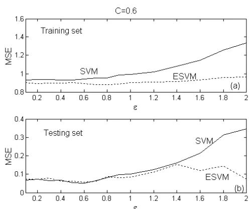
Figure 2: Influence of the error band parameterε to the performance of the SVM and ESVM for the toy example: (a) over the noise training set, and (b) over the noise-free test set. The kernel variance
and the regularization parameter C=0.6. 1
2=
[image:6.595.167.416.343.551.2]Figure 3: The experiment result of SVM for the toy example. Both the dots and circles are noisy training data. While the circles are support vectors, the dots are not. The dot curve denotes the sinc function and the solid curve indicates the kernel model. The regularization parameter C=0.6, the kernel
variance σ2 =1 and ε=0.6
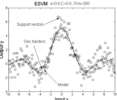
Figure 4: The experiment result of ESVM for the toy example. The circles are both training data and support vectors. The dot curve denotes the sinc function and the solid curve indicates the kernel model.
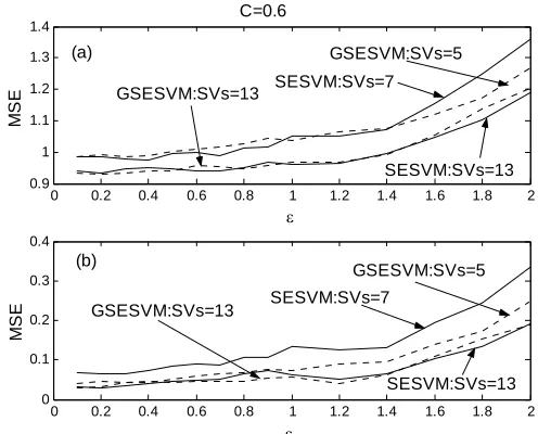
[image:7.595.200.393.418.583.2]Figure 5: Modeling performance over the noisy training set (a) and the noise-free test set (b) as function of the selected model size. For the SESVM, standard Gaussian kernel model is used with
while for the GSESVM, generalized Gaussian kernel model with tunable means and variances is used. The error band parameter
1 2 =
σ
6 . 0
=
ε , the regularization parameter C=0.6.
0 0.2 0.4 0.6 0.8 1 1.2 1.4 1.6 1.8 2
0.9 1 1.1 1.2 1.3 1.4
ε
MS
E
0 0.2 0.4 0.6 0.8 1 1.2 1.4 1.6 1.8 2
0 0.1 0.2 0.3 0.4
ε
MS
E
C=0.6
GSESVM:SVs=13
GSESVM:SVs=5
GSESVM:SVs=5
GSESVM:SVs=13
SESVM:SVs=13
SESVM:SVs=13 SESVM:SVs=7
SESVM:SVs=7 (a)
(b)
Figure 6: Influence of the error band parameterε to the performance of the SESVM and GSESVM for the toy example: (a) over the noise training set, and (b) over the noise-free test set. The regularization
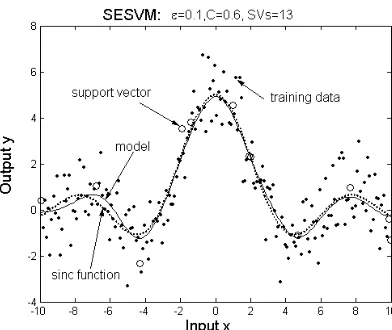
[image:8.595.168.416.396.596.2]Figure 7: The experiment result of SESVM for the toy example. Both the dots and circles are noisy training data. While the circles are support vectors, the dots are not. The dot curve denotes the sinc function and the solid curve indicates the kernel model. The regularization parameter C=0.6, the kernel
variance σ2 =1 and ε=0.1
Figure 8: The experiment result of GSESVM for the toy example. The dots are noisy training data, the circles are added support vectors while the y value is the weight of this SV. The dot curve denotes the sinc function and the solid curve indicates the kernel model. The regularization parameter C=0.6, and
1 . 0
=
[image:9.595.192.394.326.495.2]