JAMES C. PHILLIPS,1
ROSEMARY BRAUN,1
WEI WANG,1
JAMES GUMBART,1 EMAD TAJKHORSHID,1
ELIZABETH VILLA,1
CHRISTOPHE CHIPOT,2
ROBERT D. SKEEL,3 LAXMIKANT KALE´ ,3
KLAUS SCHULTEN1 1
Beckman Institute, University of Illinois at Urbana–Champaign, Urbana, Illinois 61801
2
UMR CNRS/UHP 7565, Universite´ Henri Poincare´, 54506 Vandœuvre-le`s-Nancy, Cedex, France
3
Department of Computer Science and Beckman Institute, University of Illinois at Urbana–Champaign, Urbana, Illinois 61801
Received 14 December 2004; Accepted 26 May 2005 DOI 10.1002/jcc.20289
Published online in Wiley InterScience (www.interscience.wiley.com).
Abstract:
NAMD is a parallel molecular dynamics code designed for high-performance simulation of large biomo-lecular systems. NAMD scales to hundreds of processors on high-end parallel platforms, as well as tens of processors on low-cost commodity clusters, and also runs on individual desktop and laptop computers. NAMD works with AMBER and CHARMM potential functions, parameters, and file formats. This article, directed to novices as well as experts, first introduces concepts and methods used in the NAMD program, describing the classical molecular dynamics force field, equations of motion, and integration methods along with the efficient electrostatics evaluation algorithms employed and temperature and pressure controls used. Features for steering the simulation across barriers and for calculating both alchemical and conformational free energy differences are presented. The motivations for and a roadmap to the internal design of NAMD, implemented in C⫹⫹and based on Charm⫹⫹parallel objects, are outlined. The factors affecting the serial and parallel performance of a simulation are discussed. Finally, typical NAMD use is illustrated with representative applications to a small, a medium, and a large biomolecular system, highlighting particular features of NAMD, for example, the Tcl scripting language. The article also provides a list of the key features of NAMD and discusses the benefits of combining NAMD with the molecular graphics/sequence analysis software VMD and the grid computing/collaboratory software BioCoRE. NAMD is distributed free of charge with source code at www.ks.uiuc.edu.©2005 Wiley Periodicals, Inc. J Comput Chem 26: 1781–1802, 2005
Key words: biomolecular simulation; molecular dynamics; parallel computing
Introduction
The life sciences enjoy today an ever-increasing wealth of infor-mation on the molecular foundation of living cells as new se-quences and atomic resolution structures are deposited in data-bases. Although originally the domain of experts, sequence data can now be mined with relative ease through advanced bioinfor-matics and analysis tools. Likewise, the molecular dynamics pro-gram NAMD,1together with its sister molecular graphics program VMD,2seeks to bring easy-to-use tools that mine structure infor-mation to all who may benefit, from the computational expert to the laboratory experimentalist.
The increase in our knowledge of structures is not as dramatic as that of sequences, yet the number of newly deposited structures reached a record 5000 last year. For example, the structures of pharmacologically crucial membrane proteins, which were essen-tially unknown 10 years ago, are being resolved today at a rapid
pace. Structures yield static information that can be viewed with molecular graphics software such as VMD. However, structures also hold the key to dynamic information that leads to understand-ing function and mechanism, intellectual guideposts for basic medical research. With NAMD we want to simplify access to dynamic information extrapolated from structures and provide a molecular modeling tool that can be used productively by a wide
Correspondence to: K. Schulten; e-mail: [email protected]
Contract/grant sponsor: National Institutes of Health; contract/grant number: NIH P41 RR05969
Contract/grant sponsor: Pittsburgh Supercomputer Center and the National Center for Supercomputing Applications (for supercomputer time); contract/grant number: National Resources Allocation Committee MCA93S028.
group of biomedical researchers, including particularly experimen-talists.
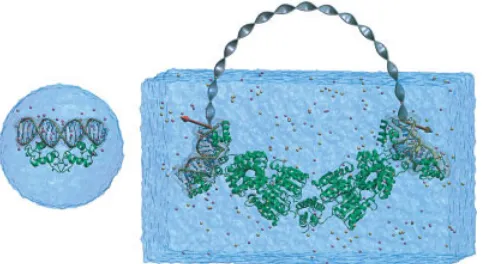
On a molecular scale, the fundamental processing units in the living cell are often huge in size and function in an even larger complex environment. Striking progress has been achieved in characterizing the immense machines of the cell, such as the ribosome, at the atomic level. Advances in biomed-icine demand tools to model these machines to understand their function and their role in maintaining the health of cells. Ac-cordingly, the purpose of NAMD is to enable high-performance classical simulation of biomolecules in realistic environments of 100,000 atoms or more. The progress made in this regard is illustrated in Figure 1. A decade ago in its first release,3,4 NAMD permitted simulation of a protein–DNA complex en-compassing 36,000 atoms,5 one of the largest simulations car-ried out at the time. The most recent release permitted the simulation of a protein–DNA complex of 314,000 atoms.6To probe the behavior of this 10-fold larger system, the simulated period actually increased 100-fold as well.
The following article on NAMD is directed to novices and experts alike. It explains the concepts and algorithms underlying modern molecular dynamics (MD) simulations as realized in NAMD, for example, the efficient numerical integration of the Newtonian equations of motion, the use of statistical mechanics methods for simulations that control temperature and pressure, the efficient evaluation of electrostatic forces through the particle-mesh Ewald method, the use of steered and interactive MD to manipulate and probe biomolecular systems and to speed up reac-tion processes, and the calculareac-tion of alchemical and conforma-tional free energy differences.
The article describes the design of NAMD and the motivation behind the design, that is, to permit continuous software develop-ment in view of ever-changing technologies, to utilize parallel computers of any size effectively via message driven computation, to run well on platforms from laptops and desktops—where NAMD is actually used most—to parallel computers with
thou-sands of processors. The article also demonstrates how the user can readily extend NAMD through the Tcl scripting language and elaborates on the strengths of NAMD in steered and interactive MD.
To demonstrate the broad utility of NAMD, the article intro-duces three typical applications as they are encountered in modern research, involving a small, an intermediate, and a large biomo-lecular system. We emphasize which features of NAMD were used and which were most helpful in completing the three modeling projects expeditiously. We also refer readers to tutorial material (available at http://www.ks.uiuc.edu/Training/Tutorials/) that has been proven helpful in NAMD training workshops and university courses. In fact, the first application presented below ubiquitin stems directly from the introductory NAMD tutorial. Other tuto-rials—for which a laptop provides sufficient computational power—introduce steered MD and simulations of membrane chan-nels, as well as the use of VMD in trajectory analysis.
Finally, a conclusion section summarizes the features of NAMD that have proven to be most relevant to nonexpert as well as expert users and describes the great benefits that NAMD gains from its close link to the widely used molecular graphics program VMD, which permits model building as well as trajectory analysis. The integration of NAMD into the grid software BioCoRE is also mentioned.
Molecular Dynamics Concepts and Algorithms
In this section we outline concepts and algorithms of classical MD simulations. In these simulations the atoms of a biopolymer move according to the Newtonian equations of motion
m␣rជ¨␣⫽⫺ ⭸
⭸rជ␣Utotal共rជ1,ជr2, . . . ,rជN兲, ␣ ⫽1, 2 . . .N, (1)
wherem␣is the mass of atom␣,rជ␣is its position, andUtotalis the total potential energy that depends on all atomic positions and, thereby, couples the motion of atoms. The potential energy, rep-resented through the MD “force field,” is the most crucial part of the simulation because it must faithfully represent the interaction between atoms, yet be cast in the form of a simple mathematical function that can be calculated quickly.
Below we introduce first the functional form of the force field utilized in NAMD. We then comment on the special problem of calculating the Coulomb potential and forces efficiently. The nu-merical integration of (1) is then explained, followed by an outline of simulation strategies for controlling temperature and pressure. In the case of such simulations, frictional and fluctuating forces are added to (1) following the principles of nonequilibrium statistical mechanics. Finally, we describe how external, user-defined forces are added to simulations to manipulate and probe biomolecular systems.
Force Field Functions
[image:2.594.47.288.82.214.2]For an all-atom MD simulation, one assumes that every atom experiences a force specified by a model force field accounting for Figure 1. Growth in practical simulation size illustrated by
the interaction of that atom with the rest of the system. Today, such force fields present a good compromise between accuracy and computational efficiency. NAMD employs a common potential energy function that has the following contributions:
Utotal⫽Ubond⫹Uangle⫹Udihedral⫹UvdW⫹UCoulomb. (2)
The first three terms describe the stretching, bending, and torsional bonded interactions,
Ubond⫽
冘
bondsikibond共ri⫺r0i兲2, (3)
Uangle⫽
冘
anglesikiangle共i⫺0i兲2, (4)
Udihedral⫽
冘
dihedrali再
kidihe关1⫹cos共nii⫺␥i兲兴,ni⫽0
kidihe共0i⫺␥i兲2n⫽0,
(5)
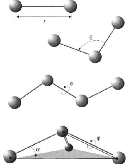
wherebondscounts each covalent bond in the system,anglesare the angles between each pair of covalent bonds sharing a single atom at the vertex, anddihedraldescribes atom pairs separated by exactly three covalent bonds with the central bond subject to the torsion angle(Fig. 2). An “improper” dihedral term governing the geometry of four planar, covalently bonded atoms is also included as depicted in Figure 2.
The final two terms in eq. (2) describe interactions between nonbonded atom pairs:
UvdW⫽
冘
i j冘
⬎i4ij
冋冉
ijrij
冊
12⫺
冉
ijrij
冊
6册
, (6)UCoulomb⫽
冘
i冘
j⬎iqiqj 40rij
, (7)
which correspond to the van der Waal’s forces (approximated by a Lennard–Jones 6 –12 potential) and electrostatic interactions, respectively.
In addition to the intrinsic potential described by the force field, NAMD also provides the user with the ability to apply external forces to the system. These forces may be used to guide the system into configurations of interest, as in steered and interactive MD (described below).
For every particle in a given context of bonds, the parameters
ki bond,r
0i, etc., for the interactions given in eqs. (3)–(5) are laid out in force field parameter files. The determination of these parame-ters is a significant undertaking generally accomplished through a combination of empirical techniques and quantum mechanical calculations;7–9the force field is then tested for fidelity in repro-ducing the structural, dynamic, and thermodynamic properties of small molecules that have been well-characterized experimentally, as well as for fidelity in reproducing bulk properties. NAMD is able to use the parameterizations from both CHARMM7 and AMBER10force field specifications.
To avoid surface effects at the boundary of the simulated system, periodic boundary conditions are often used in MD sim-ulations; the particles are enclosed in a cell that is replicated to infinity by periodic translations. A particle that leaves the cell on one side is replaced by a copy entering the cell on the opposite side, and each particle is subject to the potential from all other particles in the system including images in the surrounding cells, thus entirely eliminating surface effects (but not finite-size effects). Because every cell is an identical copy of all the others, all the image particles move together and need only be represented once inside the molecular dynamics code.
However, because the van der Waals and electrostatic interac-tions [eqs. (6) and (7)] exist between every nonbonded pair of atoms in the system (including those in neighboring cells) com-puting the long-range interaction exactly is unfeasible. To perform this computation in NAMD, the van der Waals interaction is spatially truncated at a user-specified cutoff distance. For a simu-lation using periodic boundary conditions, the system periodicity is exploited to compute the full (nontruncated) electrostatic interac-tion with minimal addiinterac-tional cost using the particle-mesh Ewald (PME) method described in the next section.
Full Electrostatic Computation
[image:3.594.320.535.85.365.2]conditions. The infinite sum of charge-charge interactions for a charge-neutral system is conditionally convergent, meaning that the result of the summation depends on the order in which it is taken. Ewald summation specifies the order as follows:12sum over each box first, then sum over spheres of boxes of increasingly larger radii. Ewald summation is considered more reliable than a cutoff scheme,13–15although it is noted that the artificial period-icity can lead to bias in free energy,16,17 and can artificially stabilize a protein that should have unfolded quickly.18
Dropping the prefactor 1/4, the Ewald sum involves the following terms:
EEwald⫽Edir⫹Erec⫹Eself⫹Esurface, (8)
Edir⫽ 1 2
冘
i,j⫽1 N
qiqj
冘
nជr
⬘erfc共兩rជi⫺rជj⫹nជr兩兲
兩rជi⫺rជj⫹nជr兩
⫺
冘
共i,j兲僆Excluded
qiqj
兩rជi⫺rជj⫹ជij兩 , (9)
Erec⫽ 1 2V
冘
mជ⫽0
exp共⫺2兩mជ兩2/2兲
兩mជ兩2
冏
冘
i⫽1 Nqiexp(2imជ 䡠rជi)
冏
2, (10)
Eself⫽⫺

冑
i冘
⫽1 Nqi2, (11)
Esurface⫽ 2 共2s⫹1兲V
冏
冘
i⫽1 N
qirជi
冏
2. (12)
Here,qiandrជiare the charge and position of atomi, respectively, andnជris the lattice vector. For an arbitrary simulation box defined by three independent base vectorsaជ1, aជ2, aជ3, one defines nជr ⫽
n1aជ1 ⫹ n2aជ2 ⫹ n3aជ3, where n1, n2, and n3 are integers. ¥⬘ denotes a summation overnជrthat excludes thenជr⫽0 term in the casei⫽j; “excluded” denotes the set of atom pairs whose direct electrostatic interaction should be excluded.ជijdenotes the lattice vector for the (i, j) pair that minimizes 兩rជi ⫺ rជj ⫹ ជij兩.  is a parameter adjusting the workload distribution for direct and recip-rocal sums.sis the dielectric constant of the surroundings of the simulation box, which is water for most biomolecular systems.V
is the volume of the simulation box.mជ is the reciprocal vector defined asmជ ⫽ m1bជ1 ⫹ m2bជ2⫹ m3bជ3, wherem1, m2, m3 are integers, and the reciprocal base vectorsbជ1, bជ2,bជ3are defined so that
aជ␣䡠bជ⫽␦␣, ␣, ⫽1, 2, 3. (13) The complementary error function erfc(x) in eq. (9) is
erfc共x兲⫽ 2
冑
冕
x ⬁e⫺t2
dt. (14)
The Ewald sum in eq. (8) has four terms: direct sum Edir, reciprocal sumErec, self-energyEself, and surface energyEsurface. The self-energy term is a trivial constant, while the surface term is usually neglected by assuming the “tin-foil” boundary condition s ⫽ ⬁, which is partly due to the dielectric constant of water (s⬇80) being much larger than 1. The Ewald sum has a freely chosen parameter, which can shift the computational load be-tween the direct sum and the reciprocal sum. For a given accuracy, the computationally optimal choice of the parameter leads to a cost proportional toN3/ 2in the standard computation, whereN is the number of charges in the system.19
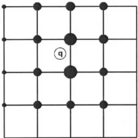
The particle–mesh Ewald (PME)20method is a fast numerical method to compute the Ewald sum. NAMD uses the smooth PME (SPME)21method for full electrostatic computations. The cost of PME is proportional toNlogNand the time reduction is signif-icant even for a small system of several hundred atoms. In PME, the parameteris chosen so that the major work load is put into the reciprocal sum while the direct sum is computed by a cost proportional toNonly. The reciprocal sum is then computed via fast Fourier transform (FFT) after an approximation is made to delegate the computation to a grid scheme. For this purpose, PME uses an interpolation scheme to distribute the charges, sitting anywhere in real space, to the nodes of a uniform grid as illustrated in Figure 3. SPME uses B-spline functions as the basis functions for the interpolation. The continuity of B-spline functions and their derivatives makes the analytical expression of forces easy to obtain, and reduces the number of FFTs by half compared to the original PME method. In SPME, approximations are made to the potential only; the force is still the exact derivative of the approx-imated potential. The strict conservation of energy resulting from the computed force is crucial and is strongly assisted by maintain-ing the symplecticness of the integrator,22 as discussed further below.
The PME method can be adopted to compute the electrostatic potential in real space and has been implemented in VMD (see Fig. 4). The feature has been used recently in a ground-breaking sim-ulation to compute transmembrane electrostatic potentials aver-aged over an MD trajectory.23This feature makes it possible today to compute average electrostatic potentials from first principles and to replace previously used heuristic potentials like those de-rived from Poisson–Boltzmann theory.
The PME method does not conserve energy and momentum simultaneously, but neither does the particle-particle/particle-mesh method24 or the multilevel summation method.25,26 Momentum conservation can be enforced by subtracting the net force from the reciprocal sum computation, albeit at the cost of a small long-time energy drift.
Numerical Integration
only how accurate it is locally, but also how efficient it is, and how well it preserves the fundamental dynamical properties, such as energy, momentum, time-reversibility, and symplectic-ness.
The time evolution of a strict Hamiltonian system is symplec-tic.22 A consequence of this is the conservation of phase space volume along the trajectory, that is, the enforcement of the Li-ouville theorem (ref. 27, p. 69). To a large extent, the trajectories computed by numerical integrators observing symplecticness rep-resent the solution of a closely related problem that is still Ham-iltonian.28Because of this, the errors, unavoidably generated by an integrator at each time step, accumulate imperceptibly slowly, resulting in a very small long-time energy drift, if there is any at all (ref. 22, theorem IX.8.1). Artificial measures to conserve en-ergy, for example, scaling the velocity at each time step so that the total energy is constant, lead to biased phase space sampling of the constant energy surface;29in contrast, there has been no evidence that symplectic integrators have this problem.
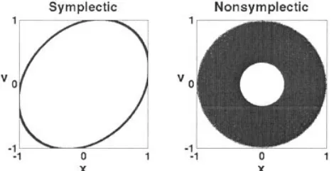
A simple example demonstrates the merit of a symplectic integrator. For this purpose, the one-dimensional harmonic oscil-lator problem has been numerically integrated, the resulting tra-jectory being shown in Figure 5. We note that the comparison is “unfair” to the symplectic method with respect to both accuracy (⌬t2local error for the symplectic method vs.⌬t5for the Runge– Kutta method, where⌬tis the time step), and computational effort (single force evaluation per time step for the symplectic method vs. four force evaluations for the Runge–Kutta method). Nevertheless, the symplectic method shows superior long-time stability.
NAMD uses the Verlet method (ref. 31, section 4.2.3) for NVE ensemble simulations. The “velocity-Verlet” method obtains the position and velocity at the next time step (rn⫹1,vn⫹1) from the current one (rn, vn), assuming the forceFn ⫽ F(rn) is already computed, in the following way:
“half-kick” vn⫹1/ 2⫽vn⫹M⫺1Fn䡠⌬t/ 2, “drift” rn⫹1⫽rn⫹vn⫹1/ 2⌬t, “compute force” Fn⫹1⫽F共rn⫹1兲,
“half-kick” vn⫹1⫽vn⫹1/ 2⫹M⫺1Fn⫹1䡠⌬t/ 2. Here,M is the mass. The Verlet method is symplectic and time reversible, conserves linear and angular momentum, and requires only one force evaluation for each time step. For a fixed time period, the method exhibits a (global) error proportional to⌬t2.
More accurate (higher order) methods are desirable if they can increase the time step per force evaluation. Higher order Runge– Kutta type methods, symplectic or not, are not suitable for biomo-lecular simulations because they require several force evaluations for each time step and force evaluation is by far the most time-consuming task in molecular dynamics simulations. Gear type predictor– corrector methods,32or linear multistep methods in gen-eral, are not symplectic (ref. 22, theorem XIV.3.1). No symplectic method has been found as yet that is both more accurate than the Verlet method and as practical for biomolecular simulations.
NAMD employs a multiple-time-stepping13,33,34 method to improve integration efficiency. Because the biomolecular interac-tions collected in eq. (2) generally give rise to several different time scales characteristic for biomolecular dynamics, it is natural to compute the slower-varying forces less frequently than faster varying ones in molecular dynamics simulations. This idea is implemented in NAMD by three levels of integration loops. The inner loop uses only bonded forces to advance the system, the middle loop uses Lennard–Jones and short-range electrostatic forces, and the outer loop uses long-range electrostatic forces. We note that the method implemented in NAMD is symplectic and time reversible.
[image:5.594.94.236.81.223.2]The longest time step for the multiple time-stepping method is limited by resonance.35When good energy conservation is needed for NVE ensemble simulations we recommend choosing 2 fs, 2 fs, and 4 fs as the inner, middle, and outer time steps if rigid bonds to hydrogen atoms are used; or 1 fs, 1 fs, and 3 fs if bonds to Figure 3. In PME, a charge (denoted by an empty circle with label
[image:5.594.311.550.526.648.2]“q” in the figure) is distributed over grid (here a mesh in two dimen-sions) points with weighting functions chosen according to the dis-tance of the respective grid points to the location of the charge. Positioning all charges on a grid enables the application of the FFT method and significantly reduces the computation time. In real appli-cations, the grid is three-dimensional.
Figure 4. Smoothed electrostatic potential of decalanine in vacuum as calculated with the PME plugin of VMD. Atoms are colored by charge (blue is positive, red is negative). The helix dipole is clearly visible from the two potential isosurfaces⫹20kBT/e (blue, left lobe) and
⫺20kBT/e(red, right lobe). [Color figure can be viewed in the online
hydrogen are flexible.36 More aggressive time steps may be used for NVT or NPT ensemble simulations, for example, 2 fs, 2 fs, and 6 fs with rigid bonds and 1 fs, 2 fs, and 4 fs without. Using multiple time stepping can increase computational effi-ciency by a factor of 2.
NVT and NPT Ensemble Simulations
A fundamental requirement for an integrator is to generate the correct ensemble distribution for the specified temperature and pressure in an appropriate way. For this purpose the Newtonian equations of motion (1) should be modified “mildly” so that the computed short-time trajectory can still be interpreted in a con-ventional way. To generate the correct ensemble distribution, the system is coupled to a reservoir, with the coupling being either deterministic or stochastic. Deterministic couplings generally have some conserved quantities (similar to total energy), the monitoring of which can provide some confidence in the simulation. NAMD uses a stochastic coupling approach because it is easier to imple-ment and the friction terms tend to enhance the dynamical stability. The (stochastic) Langevin equation37 is used in NAMD to generate the Boltzmann distribution for canonical (NVT) ensemble simulations. The generic Langevin equation is
Mv˙ ⫽F共r兲⫺␥v⫹
冑
2␥kBTM R共t兲, (15)
whereMis the mass,v⫽r˙is the velocity,Fis the force,ris the position,␥is the friction coefficient,kBis the Boltzmann constant,
Tis the temperature, andR(t) is a univariate Gaussian random process. Coupling to the reservoir is modeled by adding the fluc-tuating (the last term) and dissipative (⫺␥v term) forces to the
Newtonian equations of motion (1). To integrate the Langevin equation, NAMD uses the Bru¨nger–Brooks–Karplus (BBK) meth-od,38a natural extension of the Verlet method for the Langevin equation. The position recurrence relation of the BBK method is
rn⫹1⫽rn⫹
1⫺␥⌬t/ 2
1⫹␥⌬t/ 2共rn⫺rn⫺1兲
⫹1⫹␥1⌬t/ 2⌬t2
冋
M⫺1F(rn)⫹冑
2␥kBT⌬M Zn
册
, (16) whereZnis a set of Gaussian random variables of zero mean and variance 1. The BBK integrator requires only one random number for each degree of freedom. The steady-state distribution generated by the BBK method has an error proportional to⌬t2,39although the error in the time correlation function can have an error pro-portional to⌬t.40For stochastic equations of motion, position and velocity be-come random variables while the time evolution of the correspond-ing probability distribution function is described by the Fokker– Planck equation (ref. 37, section 2.4), a deterministic partial differential equation. The stochastic equations of motion are de-signed so that the time-independent solution to the Fokker–Planck equation is the targeted ensemble distribution. The relationship between the Langevin equation and the associated Fokker–Planck equation has been invoked, for example, in ref. 41. The theory behind deterministic coupling methods is similar, with the Li-ouville equation playing the pivotal role.42
For NPT ensemble simulations, one of the authors (J.P.) pro-posed a new set of equations of motion and implemented a nu-merical integrator in NAMD (ref. 43, pressure control section). It was inspired by the Langevin-piston method44and Hoover’s meth-od45– 47for constant pressure simulations. A recent work proposed essentially the same set of equations [the “Langevin–Hoover” method given by eqs. (5a)–(5d) in ref. 48], and proved that they generate the correct ensemble distribution. The only difference between the two is the term 1⫹d/Nfin eq. (5b) and (5d) of ref. 48, wheredis the dimension (generally 3), andNfis the number of degrees of freedom. The term d/Nf is negligible for most purposes.
Steered and Interactive Molecular Dynamics
[image:6.594.50.285.83.203.2]Biologically important events often involve transitions from one equilibrium state to another, such as the binding or dissociation of a ligand. However, processes involving the rare event of barrier crossing are difficult to reproduce on MD time scales, which today are still confined to the order of tens of nanoseconds. To address this issue, the application of external forces may be used to guide the system from one state to another, enhancing sampling along the pathway of interest. Recent applications of single-molecule exper-imental techniques (such as atomic force microscopy and optical tweezers) have enhanced our understanding of the mechanical properties of biopolymers. Steered molecular dynamics (SMD) is thein silicocomplement of such studies, in which external forces are applied to molecules in a simulation to probe their mechanical properties as well as to accelerate processes that are otherwise too slow to model. This method has been reviewed in refs. 49 –51. Figure 5. A symplectic method demonstrates superior long-time
sta-bility: the symplectic method used here is the symplectic Euler method ([22], Theorem 3.3), whose local error is proportional to⌬t2; the
nonsymplectic method used is the Runge–Kutta method ([30], sect. 8.3.3) whose local error is proportional to⌬t5. The system described
is a one-dimension harmonic oscillator. The equation of motion ismx¨
⫽ ⫺m2x, withm⫽⫽1, and initial conditionsx⫽1,
v⫽0. The exact trajectory is the unit circle. The chosen time step is⌬t⫽
With advances in available computer power, steering forces can also be applied interactively, instead of in batch mode; we call this technique Interactive Molecular Dynamics (IMD).52,53 External forces have been applied using NAMD in a variety of ways to a diverse set of systems, yielding new information about the me-chanics of proteins,54 for instance in refs. 6, 55– 67 and other studies reviewed in ref. 51. We expect that most molecular dy-namics simulations in the future will be of the steered type. This expectation stems from an analogy to experimental biophysics: although many experiments provide unaltered images of biological systems, more experiments investigate systems through well-de-signed perturbations by physical or chemical means.
SMD
Steered MD may be carried out with either a constant force applied to an atom (or set of atoms) or by attaching a harmonic (spring-like) restraint to one or more atoms in the system and then varying either the stiffness of the restraint67 or the position of the re-straint68 –70 to pull the atoms along. Other external forces or potentials can also be used, such as constant forces or torques applied to parts of the system to induce rotational motion of its domains. NAMD provides built-in facilities for applying a variety of external forces, including the automated application of moving constraints. In SMD, the direction of the applied force is chosen in advance, specified through a few simple lines in an NAMD con-figuration file. More flexible force schemes can be realized within NAMD through scripting.
As a computational technique, SMD bears similarities to the method of umbrella sampling,71,72which also seeks to improve the sampling of a particular degree of freedom in a biomolecular system; however, while umbrella sampling requires a series of equilibrium simulations, SMD simulations apply a constant or time-varying force that results in significant deviations from equi-librium. In consequence, the results of the SMD dynamics have to be analyzed from an explicitly nonequilibrium viewpoint.54SMD also permits new types of simulations that are more naturally performed and understood as out-of-equilibrium processes.
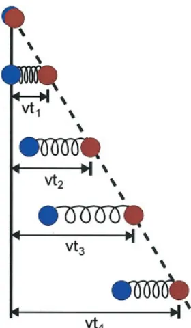
In constant-force SMD, the atoms to which the force is applied are subject to a fixed, constant force in addition to the force field potential. The affected atoms are specified through a flag in the molecular coordinates (PDB) file, and the force vector is specified in the NAMD configuration. Intermediates found through con-stant-force SMD simulations may be modeled using the theory of mean first passage times for a barrier-crossing event.73,74Typical applied forces range from tens to a thousand picoNewtons (pN).75 Constant velocity SMD simulates the action of a moving AFM cantilever on a protein. An atom of the protein, or the center of mass of a group of atoms, is harmonically restrained to a point in space that is then shifted in a chosen direction at a predetermined constant velocity, forcing the restrained atoms to follow (Fig. 6). By default, the SMD harmonic restraint in NAMD only applies along the direction of motion of the restraint point, such that the atoms are unrestrained along orthogonal vectors; it is possible, however, to apply additional restraints. As with constant force SMD, the affected atoms are specified through a flag in the PDB file; the force constant of the restraint and the velocity of the restraint point are specified in the NAMD configuration file. For a
group of atoms harmonically restrained with a force constantk
moving with velocityvin the directionnជ, the additional potential ⌬U共rជ1,rជ2, . . . ,t兲⫽
1
2k关vt⫺共Rជ共t兲⫺Rជ0兲䡠nជ兴2 (17) is applied, whereRជ(t) is the current center of mass of the SMD atoms andRជ0is their initial center of mass.nជ is a unit vector. In AFM experiments, the spring constantsk of the cantilevers are typically of the order of 1 pN/Å, so that thermal fluctuations in the position of an attached ligand, (kBT/k)1/ 2, are large on the atomic scale, for example, 6 Å. However, in SMD simulations stiffer springs (k ⬃ 70 pN/Å) are employed, leading to more detailed information about interaction energies as well as finer spatial resolution. However, due to limitations in attainable computational speeds, simulations cover time scales that are typically 105times shorter than those of AFM experiments, necessitating high pulling velocities on the order of 1 Å/ps. As a result, a large amount of irreversible work is performed during SMD simulations, which needs to be discounted to obtain equilibrium information.
A proof that equilibrium properties of a system can be deduced from nonequilibrium simulations was given by Jarzynski.76,77The second law of thermodynamics states that the average work具W典
done through a nonequilibrium process that changes a parameter of a system from0at time zero totat timetis greater than or equal to the equilibrium free energy difference between the two states specified through the final and initial values of:
⌬F⫽F共t兲⫺F共0兲ⱕ具W典, (18)
where the equality holds only if the process is quasi-static. Jar-zynski76discovered an equality that holds regardless of the speed of the process:
e⫺⌬F ⫽具e⫺W
典, (19)
where ⫽ (kBT)⫺
Application of the Jarzynski identity is comparable in effi-ciency to the umbrella sampling method.81However, the analysis involved in the SMD method is simpler than that involved in umbrella sampling in which one needs to solve coupled nonlinear equations for the weighted histogram analysis method.31,54,82,83In addition, the application of the Jarzynski identity has the advantage of uniform sampling of a reaction coordinate. Whereas in umbrella sampling a reaction coordinate is locally sampled nonuniformly proportional to the Boltzmann weight, in SMD a reaction coordi-nate follows a guiding potential that moves with a constant veloc-ity and, hence, is sampled almost uniformly (computing time is uniformly distributed over the given region of the reaction coor-dinate). This is particularly beneficial when the potential of mean force (essentially, the free energy profile along the reaction coor-dinate) contains narrow barrier regions as in ref. 62. In such cases, a successful application of umbrella sampling depends on an optimal choice of biasing potentials, whereas nonequilibrium ther-modynamic integration appears to be more robust.31 However, umbrella sampling is a general method that can be applied to a variety of reaction coordinates, including complex ones like those involved in large conformational changes in proteins.84
NAMD also provides the facility for the user to apply other types of external forces to a system. In a technique related to SMD, torques may be applied to induce the rotation of a protein domain. As with SMD, this is implemented in NAMD through a simple specification in the configuration file and does not require addi-tional programming on the part of the researcher. This technique has already been successfully used to study the rotation of the Fo
domain of ATPase.85The application of more sophisticated exter-nal forces are readily implemented through the NAMD “Tcl forces” interface, which allows the user to specify position- and time-dependent forces to be computed at each time step. This technique has recently been used to mimic the effect of membrane surface tension on a mechanosensitive channel59and to model the interaction of thelacrepressor protein (modeled in atomic-level detail) with DNA described by an elastic rod that exerts forces on the protein.6,86
IMD
By using NAMD in conjunction with the molecular graphics software VMD, steering forces can be applied in an interactive manner, rather than only in batch mode.52For this purpose, VMD is linked to a NAMD simulation running on the same machine or a remote cluster. This arrangement permits an investigator to view a running simulation and to apply forces based on real-time mation about the progress of the simulation (such as visual infor-mation or force feedback through a haptic device). The researcher is then able to explore the mechanical properties of the system in a direct, hands-on manner, using her scientific intuition to guide the simulation via a mouse or haptic device. This method has already been used in biomolecular research, for instance, to study the selectivity and regulation of the membrane channel protein GlpF and the enzyme glycerol kinase.53Setting up an IMD sim-ulation is a straight-forward process that can be done on any computer.
[image:8.594.96.236.78.318.2]The IMD haptic interface52consists of three primary compo-nents: a haptic device to provide translational and orientational input as well as force feedback to the user’s hand; NAMD to calculate the effect of applied forces via molecular dynamics; and VMD to display results (Fig. 7). VMD communicates with the haptic device via a server87that controls the haptic environment experienced by the user, as described in ref. 52. The scheme of splitting the haptic, visualization, and simulation components into three communicating, asynchronous processes has been employed successfully,52,88and permits all three components to run at top speed, maximizing the responsiveness of the system. IMD requires Figure 6. Constant velocity pulling in a one-dimensional case. The
dummy atom is colored red, and the SMD atom blue. As the dummy atom moves at constant velocity, the SMD atom experiences a force that depends linearly on the distance between both atoms. [Color figure can be viewed in the online issue, which is available at www. interscience.wiley.com.]
[image:8.594.321.531.537.688.2]efficient network communication between the visualization front-end and the MD back-front-end. Although the network bandwidth re-quirements for performing IMD are quite low relative to the computational demands, latency is a major concern as it has a direct impact on the responsiveness of the system. IMD uses custom networking code in NAMD and VMD to transfer atomic coordinates and steering forces efficiently.
To make molecular motion as described by MD perceptible to the IMD user through the haptic device, the quantities arising in the generic equation of motion governing the molecular response (represented below by Roman characters) and the haptic response (denoted by Greek characters),
md
2x
dt2⫽f,
d2
d2⫽ (20)
must be related through suitable scaling factors. Molecular motion probed is typically extended over distances ofx⫽1 Å, molecular time scales covered are typically t ⫽ 1 ps, and external forces acting on molecular moieties should not exceedf⫽1 nN so as not to overwhelm inherent molecular forces. By contrast, the haptic device is characterized by length resolution of⫽1 cm and can generate a force of ⫽ 1 N or more; t ⫽ 1 ps of dynamics requires⫽1 s or more to compute. The interface between the haptic device and NAMD thus introduces the scaling factors
Sx⫽/x⫽108, St⫽/t⫽1012, Sf⫽/f⫽109, (21) Multiplying the molecular equation of motion in eq. (20) by the factorSfSx/St2gives
SfSx
St 2 m
d2x
dt2⫽Sfm
d2
d2⫽
SfSx
St 2 f⫽
Sx
St
2. (22)
From this we can conclude
SfSt2
Sx
md
2
d2⫽. (23)
Comparison with the haptic equation of motion in eq. (20) suggests that the effective mass felt by the haptic device, and hence, by the user is
⫽SfSt2
Sx
m. (24)
The molecular moieties to be moved through external forces have typical masses of (e.g., for glycerol moved through a membrane channel53) ofm⫽180 amu orm⬇3⫻10⫺25kg. From eq. (21) we conclude then that the effective mass felt by the user through the haptic device is 3 kg; the user does not sense strong inertial effects, and can readily manipulate the biomolecular system. IMD can also be carried out without force feedback, using a standard mouse to steer the simulated system.
To assist users of NAMD with IMD, AutoIMD89 has been developed. AutoIMD permits the researcher to use the graphical
interface provided by VMD to run an MD simulation based on a selection of atoms. The simulation can then be visualized in real time in the VMD graphics window. Forces may be applied with either a mouse or a haptic device by the user (as described above), or statically as in traditional SMD. Rather than carrying out a simulation of the entire molecule, AutoIMD performs a rapid MD simulation by dividing the system into three parts: a “molten zone,” where the atoms are allowed to move freely; a surrounding “fixed zone,” in which the atoms are included in the simulation (and exert forces on the molten zone), but are held fixed; and an “excluded zone,” which is entirely disregarded in the AutoIMD simulation. In this way, AutoIMD may be used to inspect and perform energy minimizations on parts of the system that have been manipulated (e.g., through mutations or IMD), giving the researcher real-time feedback on the simulation.
SMD and IMD simulations differ in fundamental ways, and may be fruitfully combined. In SMD, the specification of the external forces is developed based on the researcher’s understand-ing of the biological and structural properties of the system. The SMD simulation is carried out with the weakest force possible to induce the necessary change in an affordable length of simulation time, and the analysis of the simulation data relates the force applied to the progress of the system along the chosen reaction path. In contrast, IMD simulations are unplanned, allowing the researcher to toy with the system, exploring the degrees of free-dom. Because the simulations need to be rapid— completed in minutes rather than days or weeks—the applied forces are ex-tremely large, and the simulations are too rough to produce data suitable for an accurate analysis of molecular properties. The techniques can be combined: in the first stage, the researcher uses IMD to generate and test hypotheses for reaction mechanisms or to accelerate substrate transport, docking, and other mechanisms that are difficult to cast into numerical descriptions; in the second stage, the researcher carries out further MD or SMD simulations building on the hypothesized mechanisms or configurations from the IMD investigation.
Free Energy Calculations
In addition to propagating the motion of atoms in time, MD can also be used to generate an ensemble of configurations, from which thermodynamic quantities like free energy differences,⌬F, can be computed. In a nutshell, there are three possible routes for the calculation of⌬F: (1) estimate the relevant probability distribu-tion,[U(rជ1, . . . ,rជN)], from which a free energy difference may be inferred via⫺1/ln[U(rជ1, . . . ,rជN)]/0, where0denotes a normalization term: (2) compute the free energy difference di-rectly; and (3) calculate the free energy derivative,d⌬F()/d, along some order parameter (collective coordinate),, consistent with an average force,90and integrate the latter to obtain⌬F.
we shall focus on the second and the third classes of approaches for determining free energy differences.
The first approach, available in NAMD since version 2.4, is free energy perturbation (FEP),91an exact method for the direct computation of relative free energies. FEP offers a convenient framework for performing “alchemical transformations,” or in silicosite-directed mutagenesis of one chemical species into an-other.
Description of intermolecular association or intramolecular de-formation in complex molecular assemblies requires an efficient computational tool, capable of rapidly providing precise free en-ergy profiles along some ordering parameter,, in particular when little is known about the underlying free energy behavior of the process. A fast and accurate scheme, pertaining to the third cate-gory of methods, is introduced in NAMD version 2.6 to determine such free energy profiles, ⌬F(). This scheme relies upon the evaluation of the average force acting along the chosen order parameter,, in such a way that no apparent free energy barrier impedes the progress of the system along the latter.92,93
The efficiency of the free energy algorithm represents only one facet of the overall performance of the free energy calculation, which to a large extent, relies on the ability of the core MD program to supply configurations and forces in rigorous thermo-dynamic ensembles and in a time-bound fashion. The methodology described hereafter has been implemented in NAMD and operates with nearly no extra cost compared to a standard MD simulation.
Alchemical Transformations
Contrary to the worthless piece of lead in the hands of the pro-verbial alchemist, the potential energy function of the computa-tional chemist is sufficiently malleable to be altered seamlessly, thereby allowing the thermodynamic properties of a system to be related to those of a slightly modified one, such as a chemically modified protein or ligand, through the difference in the corre-sponding intermolecular potentials.
The free energy difference between a reference state,a, and a target state, b, can be expressed in terms of the ratio of their corresponding partition functions. Using the well-known relation-ship between partition functionZand free energyF,Z⫽exp[⫺F/
k8T], along with the propertyZ⫽ZkinZpotwhereZkinandZpotare the partition functions for kinetic and potential energy, respec-tively, one can expressF⌬a3b⫽ Fb ⫺Fa as:
⌬Fa3b⫽⫺ 1 ln
兰exp关⫺Ub共rជ1, . . . ,rជN兲兴drជ1. . .drជN 兰exp关⫺Ua共rជ1, . . . ,rជN兲兴drជ1. . .drជN
. (25)
HereUaandUbare the potential energy functions for statesaand
b, respectively. One can write eq. (25) ⌬Fa3b ⫽⫺(1/)ln{兰 exp[⫺(Ub()⫺Ua())]exp[⫺Ua()]dx/兰exp[⫺Ua()]dx} where ⫽rជ1, . . . , rជN. Defining the average, Boltzmann-weighted relative to the potentialUa, that is, weighted over configurations representa-tive of the reference state a, 具f典a ⫽ 兰f()exp[⫺Ua()]dx/兰 exp[⫺Ua()]dx, one can state:
⌬Fa3b⫽⫺ 1
ln具exp兵⫺关Ub共rជ1, . . . ,ជrN兲⫺Ua共rជ1, . . . ,rជN兲兴其典a. (26)
This is the celebrated FEP equation.91In principle, eq. (26) is
exactin the limit of infinite sampling. In practice, however, on the basis of finite-length simulations, it only provides accurate esti-mates for small changes betweenaandb. This condition does not imply that the free energies characteristic ofaandbbe sufficiently close, but rather that the corresponding configurational ensembles overlap to a large degree to guarantee the desired accuracy. For example, although the hydration free energy of benzene is only ⫺0.4 kcal/mol, insertion of a benzene molecule in bulk water constitutes too large a perturbation to fulfill the latter requirement in a single-step transformation. If such is not the case, the pathway connecting stateato statebis broken down intoNintermediate, not necessarily physical states,k(a⬅ 1⫽ 0 andb⬅ N⫽ 1), so that the Helmholtz free energy difference reads:
⌬Fa3b⫽⫺ 1 k
冘
⫽1N⫺1
ln具exp兵⫺关U共rជ1, . . . ,rជN;k⫹1兲
⫺U共rជ1, . . . ,ជrN;k兲兴其典k. (27)
Here the potential energy is not only a function of the spatial coordinates, but also of the parameterthat connects the reference and the target states. Perturbation of the chemical system by means ofk may be achieved by scaling the relevant nonbonded force field parameters of appearing, vanishing, or changing atoms, in the spirit of turning lead into gold.
In NAMD, the topologies characteristic of the initial state,a, and the final state,b, coexist, yet without interacting. This implies that, as a preamble to the free energy calculation, a hybrid topol-ogy has to be defined with an appropriate exclusion list to prevent interactions between those atoms unique to state a and those unique to stateb. In lieu of altering the nonbonded parameters, the interaction of the perturbed molecular fragments with their envi-ronment is scaled as a function ofk:
U共rជ1, . . . ,rជN;k兲⫽kUb共rជ1, . . . ,rជN兲
⫹共1⫺k兲Ua共rជ1, . . . ,rជN兲. (28)
This scheme is referred to as the dual-topology paradigm.94 In a number of MD programs, FEP is implemented as an extra layer, implying that free energy differences are computeda pos-teriori by looping over a previously generated trajectory. In NAMD, the potential energies representative of the reference state, k, and the target state,k⫹1, are evaluated concurrently “on the fly” at little additional cost and the ensemble average of eq. (27) is updated continuously.
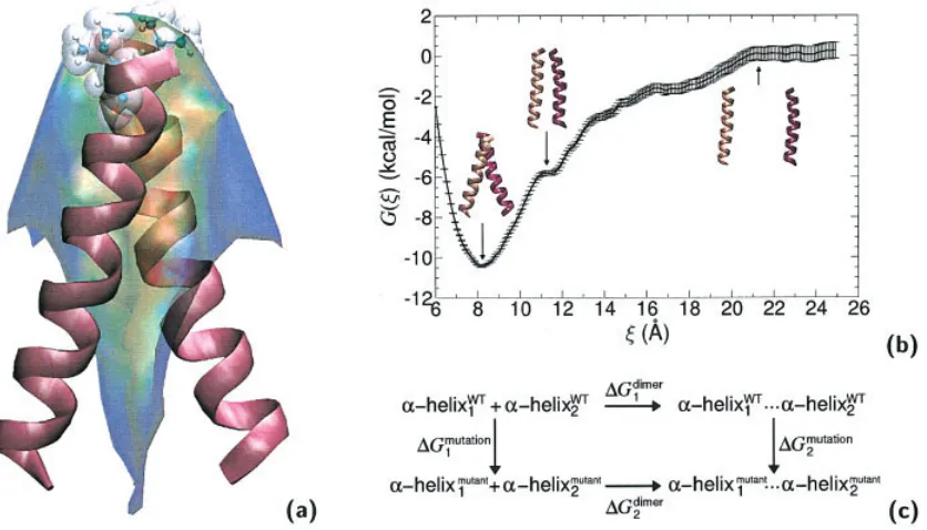
0.5 kcal/mol in the free and in the bound state, respectively, which, put together, corresponds to a net free energy change of ⫹1.0 ⫾ 0.6 kcal/mol (experimental estimate:95 ⫹1.1 ⫾ 0.1 kcal/mol). The second point mutation, I76A, led to a free energy change of⫺4.9⫾0.3 and⫺8.4⫾0.4 kcal/mol, in the single helix and in the dimer, respectively, that is, a net change of⫹1.4 ⫾0.5 kcal/mol (experimental estimate:95⫹1.7⫾0.1 kcal/mol). Aside from the remarkable agreement between the-ory and experiment, these free energy calculations confirm that replacement of bulky nonpolar side chains like leucine or isoleucine by alanine disrupts the␣-helical dimer through a loss of van der Waals interactions.96
Overcoming Free Energy Barriers Using an Adaptive Biasing Force
The sizeable number of degrees of freedom described explicitly in statistical simulations of large molecular assemblies, in particular those of both chemical and biological interest, rationalizes the need
for a compact description of thermodynamic properties. Free en-ergy profiles offer a suitable framework that fulfills this require-ment by providing the dependence of the free energy on the chosen degrees of freedom. Determination of such free energy profiles, under thesine qua noncondition that some key degree of freedom , for example, a reaction coordinate, can be defined, however, remains a daunting task from the perspective of numerical simu-lations. In the context of Boltzmann sampling of the phase space, overcoming the high free energy barriers that separate thermody-namic states of interest is a rare event that is unlikely to occur on the time scales amenable to MD simulation.
[image:11.594.92.510.82.321.2]An important step forward on the road towards an optimal sampling of the phase space along a chosen collective coordinate, , has been made recently. In a nutshell, this new method relies on the continuous application of a dynamically adapted biasing force that compensates the current estimate of the free energy, thus virtually erasing the roughness of the free energy landscape as the system progresses along.92To reach this goal, the average force
Figure 8. Homodimerization of the transmembrane (TM) domain of glycophorin A (GpA): (a) Contact surface of the two␣-helices forming the TM domain of GpA. The strongest contacts are observed in the heptad of amino acids, Leu75, Ile76, Gly79, Val80, Gly83, Val84, and Thr87. Residue Leu75, which
participates in the association of the two ␣-helices through dispersive interactions, is featured as transparent van der Waals spheres. (b) Free energy profile delineating the reversible dissociation of the two␣-helices, obtained using an adaptive biasing force. The ordering parameter,, corresponds to the distance separating the center of mass of the TM segments. The entire pathway was broken down into 10 windows, in which up to 15 ns of MD sampling was performed, corresponding to a total simulation time of 125 ns. (c) Thermodynamic cycle utilized to perform the “alchemical transformation” of residues Leu75
and Ile76into alanine, demonstrating the participation of these amino acids in the homodimerization of the
two␣-helices. The left vertical leg of the cycle represents the transformation in a single␣-helix from the wild-type (WT) to the mutant form. The right vertical leg denotes a simultaneous point mutation in the two interacting␣-helices. Using the notation of the figure, the free energy difference arising from this perturbation is equal to⌬G2mutation⫺2⌬G1mutation. Each leg of the thermodynamic cycle consists of 50
acting on,具F典, is evaluated from an unconstrained MD simu-lation:93
dA共兲 d ⫽
冓
⭸U(rជ1, . . . ,rជN)
⭸ ⫺ 1 
⭸ln兩J兩
⭸
冔
⫽⫺具F典, (29)where兩J兩 denotes the determinant of the Jacobian for the trans-formation from Cartesian to generalized coordinates, which is a necessary modification of metric, given that {rជ1, . . . , rជN} and are not independent variables. The specific form of 兩J兩 is an inherent function of the coordinate, , chosen to advance the system.
In the course of the simulation in NAMD, the force,F, acting along the ordering parameter,, is accrued in small bins, thereby supplying an estimate of the derivativedA()/d. The so called adaptive biasing force (ABF),FជABF⫽ ⫺具F
典ⵜជr, is determined in such a way that, when applied to the system, it yields a Hamiltonian in which no average force is exerted along. As a result, all values ofare sampled with an equal probability, which in turn, dramatically improves the accuracy of the calculated free energies. The approach further entails that progression of the system alongis fully reversible and limited solely by its self-diffusion properties. At this stage, it should be clearly understood that whereas the ABF method enhances sampling along , its ability to supply a perfectly uniform probability distribution of the system over the entire range of values may be impeded by possible orthogonal degrees of freedom.
We have chosen to introduce the average force method in NAMD within the convenient framework ofunconstrainedMD,93in which the coordinate,is unconstrained, but other degrees of freedom, such as bond lengths, can be constrained. Either constraint forces must be taken into account inF, as they are in NAMD version 2.6, or it will be crucial to ascertain that no Cartesian coordinate appears simulta-neously in a constrained degree of freedom and in the derivative ⭸U(rជ1, . . . ,rជN)/⭸of eq. (29).
The implementation of the ABF scheme in NAMD provides reaction coordinates such as a distance between subgroups of atoms or length along a specified direction in cartesian space. Previous appli-cations include, the intramolecular folding of a short peptide, the partitioning of small solutes across an aqueous interface, and the intermolecular association of neutral and ionic species.92,93
The ␣-helical dimerization of GpA represents an interesting application of the method, whereby the reversible dissociation— rather than the association, for obvious cost-effectiveness rea-sons—is carried out, using the distance separating the center of mass of the trans-membrane segments as the reaction coordinate. The free energy profile characterizing this process is shown in Figure 8, and features a deep minimum at 8.2 Å, which corre-sponds to the native, close packing of the␣-helices.
As the trans-membrane segments move away from each other, helix– helix interactions are progressively disrupted, in particular in the crossing region, thus causing an abrupt in-crease of the free energy, accompanied by a tilt of the two ␣-helices towards an upright orientation. As the distance be-tween the two trans-membrane segments further increases, the free energy profile levels off at 21 Å, a separation beyond which the dimer is fully dissociated.
A valuable feature offered by NAMD lies in the possibility to evaluatea posteriorielectrostatic and van der Waals forces from an ensemble of configurations. Projection of these forces onto the coordinate, and subsequent integration of the former provides a deconvolution of the complete free energy profile in terms of helix– helix and helix–solvent contributions.
Analysis of these contributions reveals two regimes in the association process, driven at large separation by the solvent, which pushes the␣-helices together, and at short separation by van der Waals interactions that favor native contacts.96
NAMD Software Design
Just as the intelligent car buyer looks under the hood to understand the performance and longevity of a particular vehicle, we now direct the attention of the reader and potential NAMD user to a few design and implementation details that contribute to the flexibility and performance of NAMD.
Goals, Design, and Implementation
NAMD was developed to enable ambitious MD simulations of biomolecular systems, employing the best technology available to provide the maximum performance possible to researchers. In the past decade simulation size and duration have increased dramati-cally. Ten years ago a simulation of 36,000 atoms over 100 ps as reported in ref. 5 was considered very advanced. Today, this status is reserved for simulations of systems with more than 300,000 atoms for up to 100 ns as reported in refs. 6, 23, and 55. The progress made is illustrated in Figure 1, comparing the sizes of systems reported in refs. 5 and 6. This 1000-fold increase in capability (10-fold in atom count and over 100-fold in simulation length) has been partially enabled by advances in processor per-formance, with clock rate increases leading the way. However, substantial progress has also resulted from exploiting the factor of 100 or more in performance available through the use of massively parallel computing, coordinating the efforts of numerous proces-sors to address a single computation.
Scientific computing is also facing the perennial “software crisis” that has stalked business information systems for decades. The seminal book by Allen and Tildesley97could dedicate a few pages of an appendix to writing efficient FORTRAN-77 code and consider the reader adequately informed. Developing modern high-performance software, however, requires knowledge of ev-erything from parallel decomposition and coordination libraries to the relative cost of accessing different levels of cache memory. The design of more complex algorithms and numerical methods has ensured that any useful and successful program is likely to outlive the machine for which it is originally written, making portability a necessity. Software is also likely to be used and extended by persons other than the original author, making code readability and modifiability vital.
Software maintenance activities such as porting and modifica-tion account for the majority of the cost and effort associated with a program during its lifetime. These issues have been addressed in the development of object-oriented software design, in which the programmer breaks the program into “objects” comprising closely-related data (such as thex, y, andzcomponents of a vector) and the operations that act on it (addition, dot product, cross product, etc.). The objects may be arranged into hierarchies of classes, and an object may contain or refer to other objects of the same or different classes. In this manner, large and complex programs can be broken down into smaller components with defined interfaces that can be implemented independently. NAMD is implemented in C⫹⫹, the most popular and widely supported programming lan-guage providing efficient support for these methods.
Methodology for the development of parallel programs is far from mature, with automatically parallelizing compilers and lan-guages still quite limited and most programmers using the Mes-sage Passing Interface (MPI) libraries in combination with C, C⫹⫹, or Fortran. Although the acceptance of MPI as a crossplat-form standard for parallel software has been of great benefit, the burden on the programmer remains. The first task is to decompose the problem, which is often simplified by assuming that the pro-cessor count is a power of two or has factors corresponding to the dimensions of a large three-dimensional array. MPI programming then requires the explicit sending and receiving of arrays between processors, much like directing a large and complex game of catch. NAMD is based on the Charm⫹⫹parallel programming sys-tem and runtime library.98In Charm⫹⫹, the computation is de-composed into objects that interact by sending messages to other objects on either the same or remote processors. These messages are asynchronous and one sided, that is, a particular method is invoked on an object whenever a message arrives for it rather than having the object waste resources while waiting for incoming data. Thismessage-driven object programming style effectively hides communication latency and is naturally tolerant of the system noise that is found on workstation clusters. Charm⫹⫹ also sup-ports processor virtualization,99 allowing each algorithm to be written for an ideal, maximum number of parallel objects that are then dynamically distributed among the actual number of proces-sors on which the program is run. Charm⫹⫹ provides these benefits even when it is implemented on top of MPI, an option that allows NAMD to be easily ported to new platforms.
The parallel decomposition strategy used by NAMD is to treat the simulation cell (the volume of space containing the atoms) as
a three-dimensional patchwork quilt, with eachpatchof sufficient size that only the 26 nearest-neighboring patches are involved in bonded, van der Waals, and short-range electrostatic interactions. More precisely, the patches fill the simulation space in a regular grid and atoms in any pair of non-neighboring patches are sepa-rated by at least the cutoff distance at all times during the simu-lation. Each hydrogen atom is stored on the same patch as the atom to which it is bonded, and atoms are reassigned to patches at regular intervals. The number of patches varies from one to several hundred and is determined by the size of the simulation indepen-dently of the number of processors. Additional parallelism may be generated through options that double the number (and have the size) of patches in one or more dimensions.
When NAMD is run, patches are distributed as evenly as possible, keeping nearby patches on the same processor when there are more patches than processors, or spreading them across the machine when there are not. Then, a (roughly 14 times) larger number of compute objects responsible for calculating atomic interactions either within a single patch or between neighboring patches is distributed across the processors, minimizing commu-nication by grouping compute objects responsible for the same patch together on the same processors. At the beginning of the simulation, the actual processor time consumed by each compute object is measured, and this data is used to redistribute compute objects to balance the workload between processors. This mea-surement-based load balancing100contributes greatly to the paral-lel efficiency of NAMD.
Using forces calculated by compute objects, each patch is responsible for integrating the equations of motion for the atoms it contains. This can be done independently of other patches, but occasionally requires global data affecting all atoms, such as a change in the size of the periodic cell due to a constant pressure algorithm. Although the integration algorithm is the clearly visible “outer loop” in a serial program, NAMD’s message-driven design could have resulted in much obfuscation (as was experienced even in the simpler NAMD 1.X4). This was averted by using Charm⫹⫹ threads to write a top-level function that is called once for each patch at program start and does not complete until the end of the simulation.10This design has allowed pressure and temperature control methods and even a conjugate gradient minimizer to be implemented in NAMD without writing any new code for parallel communication.
Tcl Scripting Interface