CMA-PAES : Pareto archived evolution strategy using
covariance matrix adaptation for Multi-Objective
Optimisation
ROSTAMI, Shahin and SHENFIELD, Alex
<http://orcid.org/0000-0002-2931-8077>
Available from Sheffield Hallam University Research Archive (SHURA) at:
http://shura.shu.ac.uk/8312/
This document is the author deposited version. You are advised to consult the
publisher's version if you wish to cite from it.
Published version
ROSTAMI, Shahin and SHENFIELD, Alex (2012). CMA-PAES : Pareto archived
evolution strategy using covariance matrix adaptation for Multi-Objective
Optimisation. In: 12th UK Workshop on Computational Intelligence (UKCI) 2012.
IEEE, 1-8.
Copyright and re-use policy
See
http://shura.shu.ac.uk/information.html
Sheffield Hallam University Research Archive
CMA-PAES: Pareto Archived Evolution Strategy
using Covariance Matrix Adaptation for
Multi-Objective Optimisation
Shahin Rostami
School of Engineering Manchester Metropolitan UniversityManchester, United Kingdom Email: [email protected]
Dr Alex Shenfield
School of Engineering Manchester Metropolitan UniversityManchester, United Kingdom Email: [email protected]
Abstract—The quality of Evolutionary Multi-Objective Optim-isation (EMO) approximation sets can be measured by their proximity, diversity and pertinence. In this paper we introduce a modular and extensible Multi-Objective Evolutionary Algorithm (MOEA) capable of converging to the Pareto-optimal front in a minimal number of function evaluations and producing a diverse approximation set. This algorithm, called the Covariance Matrix Adaptation Pareto Archived Evolution Strategy (CMA-PAES), is a form of (µ+λ) Evolution Strategy which uses an online archive of previously found Pareto-optimal solutions (maintained by a bounded Pareto-archiving scheme) as well as a population of solutions which are subjected to variation using Covariance Matrix Adaptation. The performance of CMA-PAES is compared to NSGA-II (currently considered the benchmark MOEA in the literature) on the ZDT test suite of bi-objective optimisation problems and the significance of the results are analysed using randomisation testing.
Index Terms—Meta-heuristics, Multi-Objective Optimisation, Multi-Objective Evolutionary Algorithm, Evolution Strategy, Ad-aptive Grid Archiving, Covariance Matrix Adaptation, Diversity preservation, Pareto-optimal solutions
I. INTRODUCTION
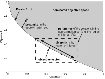
The quality of Evolutionary Multi-Objective Optimisation (EMO) candidate solution sets can be measured by their proximity, diversity and pertinence. Proximity is a measure of the distance between the approximation set and the true Pareto-optimal front1whilst diversity is a measure of the distribution of solutions along that front in multi-objective space. An ideal multi-objective optimiser converges to solutions that are uniformly spread along the true Pareto-optimal front [3]. In real-world optimisation problems this approximation set must also be pertinent [4] (that is relevant to the preferences expressed by the Decision Maker (DM)). A good Multi-Objective Evolutionary Algorithm (MOEA) satisfies these goals adequately, presenting the DM with an approximation set of diverse trade-off solutions within the search space of
1This notion of “Pareto” optimality was originally proposed by Francis
Edgeworth in 1881 [1] and was later developed by the Italian economist Vilfredo Pareto in 1896 who used the concept in his studies of economic efficiency and income distribution [2].
[image:2.612.330.548.295.459.2]their specified Region Of Interest (ROI). These measures of performance have been illustrated in figure 1.
Figure 1. Proximity, diversity, and pertinence characteristics in an approx-imation set for a bi-objective problem.
preservation in MOEAs, beginning with an introduction to diversity preservation in MOEAs, an overview of the trade-off between proximity and diversity, and concluding with an overview of methods of diversity preservation including those used in the algorithms compared in the experiment.
Methods are described in section IV with a description of CMA-PAES, an overview of the ZDT suite of test functions and the difficulties each function imposes, the performance metrics and randomisation testing used to produce the results, and the configurations of the algorithms compared. Section V contains the results and observations from the proximity and diversity performance analysis. Section VI concludes the paper with the some final observations and recommendations for further work.
II. EVOLUTIONARYMULTI-OBJECTIVEOPTIMISATION
A. Evolutionary Algorithms
Evolutionary Computation (EC) refers to a methodology concerning adaptive search and optimisation techniques, de-rived from the mechanics of natural selection [7] and modern genetics [8]. EC is a sub-field of Computational Intelli-gence (CI) alongside other biologically inspired computing techniques such as Artificial Neural Networks (ANN) and Artificial Immune Systems (AIS), and as an interdisciplinary field of research, it brings together theories of evolutionary biology, computation, mathematics and physics. The emer-gence of EC can be traced to the early 1930s when the geneticist Sewall Wright [9] provided mathematicians with the notion that evolution is a form of computation. Inspired by these concepts, John Holland [10] laid down the foundations for Evolutionary Algorithms (EA), based on the adaptive processes of natural systems. The fundamentals of an EA are population-based stochastic variation and selection, with an emphasis on robustness [11], and were primarily used in single-objective optimisation problems when minimising or maximising only one objective function.
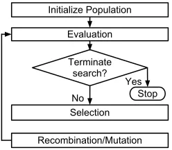
The flow of a general and basic EA is shown in figure 2. The optimisation process begins by generating an initial population of random candidate solutions which are then evaluated using objective functions and assigned a fitness value based on the objective value and potentially other values. A termination criteria is then checked to see if the maximum number of generations has been reached or any of the solutions are satisfactory to stop the optimisation process, otherwise it will continue onto selection of the fittest individuals from the population. The selected candidate solutions are then used for recombination to exploit the best solution information, and mutation to allow for exploration of the search space beyond the available solution information present in the population and prevent the possibility of getting stuck in a local optima. Ideas of solving real-valued optimisation problems using the evolutionary process were considered by Rechenberg [12] and Schwefel [13] which resulted in the formation of a set of algorithms named “Evolution Strategies” (ES). The ES process differed from other EA methods in two ways: ESs used real-encoded parameter values; and they did not use
Initialize Population
Evaluation
Terminate search?
Stop
Recombination/Mutation Yes
Selection No
Figure 2. General flow diagram of a basic Evolutionary Algorithm.
recombination operators, instead the variation of solutions during the optimisation process is driven entirely by mutation. ESs typically came in two forms: two-member ESs (1 + 1), in which a single parent is used to create a single offspring using a mutation operator; and multi-member ESs (µ+λ) or (µ, λ), in which a population of µ solutions is used to createλoffspring solutions using a mutation operator. In the “plus” variation of the multi-member ES, both parent and offspring populations are considered in selection for the next parent population, whereas in the “comma” variation, only the offspring population is used, making the (µ+λ) an elitist procedure.
The Covariance Matrix Adaptation Evolutionary Strategy (CMA-ES) is a state-of-the-art single objective ES, first intro-duced in [5] and later improved upon in [14] and [15]. It has been shown to perform extremely well across a broad range of problems in the continuous domain [16]. One of the key beneficial properties of CMA-ES is the speed at which it can find good approximations to (and in many cases the actual value of) the global minimum. It is also extremely robust to the initial parameter set used due to its self adaptive nature.
B. Multi-Objective Optimisation
Multi-Objective Optimisation (MOO), refers to problems with two or more objective functions. This is frequently the case with real-world problems in search and optimisation which naturally involve multiple objectives or multiple cri-teria [3]. A fundamental difference between single-objective optimisation and MOO is that in single-objective optimisation problems, the objective is to find a single solution which is the global optimum in the entire search space. However, in MOO a solution is actually an approximation set of candidate solutions which offer trade-offs between the multiple objectives, where an improvement in one objective value will result in a decline in one or more of the others. This notion of “optimum” solutions is called Pareto optimality.
x= (x1, x2, . . . , xn) (1)
optimise fm(x), m= 1,2, . . . , M;
subject to gj(x)≥0, j = 1,2, . . . , J;
hk(x) = 0, k= 1,2, . . . , K;
x(L)i ≤xi≤x (U)
i i= 1,2, . . . , n;
[image:3.612.377.501.53.161.2]f(x) = (f1(x), f2(x), . . . , fM(x)) (3)
A solution x is defined in (1) as a vector of n decision
variables. In formula (2) we see a MOO problem in its general form, taken from [3]. There are M objective functions each with the definition in formula (3), these objective functions can be either minimised or maximised. The constraint functions
gj(x) and hk(x) impose inequality and equality constraints
that must be satisfied by a solutionxif it is to be considered a feasible solution. Another condition deciding the feasibility of a solution regards the adherence of a solution xto values between the lower x(L)i and upperx
(U)
i boundaries within the
decision space.
C. Multi-Objective Evolutionary Algorithms
MOO problems had previously been solved by being treated as single-objective problems by using techniques such as the weighted sum approach [17]. In this approach different
weights are assigned to each objective function based on their importance and their priority. These weighted objectives are then aggregated into a singleweighted sum, allowing the use of conventional optimisation techniques to solve the problem. A major disadvantage of using the weighted sum approach and other conventional MOO approaches is that by design they can only produce a single candidate solution per execution, and therefore require multiple executions to generate a set of trade-off solutions.
In contrast, MOEAs have inherited beneficial properties from the principles on which they are based. EAs are suitable for solving MOO problems, due to being population based and therefore being able to generate and exploit more than a single solution per generational iteration, this allows them to find several solutions in the Pareto optimal set in a single algorithm execution [18]. In addition, MOEAs do not require auxiliary or derivative information about the problem, do not require aggregation of objectives into a single objective, and are less susceptible to the shape or continuity of the Pareto-optimal front.
Within the last decade there have been major advances in the field of EMO. Whilst the first generation of Pareto-based MOEAs (such as the Multi-Objective Genetic Algorithm (MOGA), Niched Pareto Genetic Algorithm (NPGA), and Non-dominated Sorting Genetic Algorithm (NSGA)) were characterised by the simplicity of the algorithms and lack of rigorous methodology for their analysis [19], the latest gener-ation of MOEAs have focussed on efficient convergence to the whole of the true Pareto-optimal front. This is accomplished by incorporatingelitism(ensuring that the best solutions are never
lost during the optimisation process) and advanced methods for the preservation of diversity (to ensure a good spread of solutions across the whole Pareto-optimal front) into the selection-for-survival process. There are two main strategies for incorporating elitism into EMO algorithms – maintaining an archive of non-dominated solutions and using a (µ+λ) type selection-for-survival mechanism.
The archiving approach to elitism is typified by PAES which proposes a conceptually simple MOEA capable of producing a diverse approximation set with close proximity to the true Pareto-optimal front [20]. PAES uses a (1 + 1) ES in conjunction with a novel AGA scheme. This bounded Pareto archive stores only non-dominated solutions that are discovered during the search and a non-dominated candidate solution is compared to the archive before it is accepted as a current solution. Once the archive has reached capacity, a grid system (whereby the search space currently covered by non-dominated solutions is divided up into a set number of partitions) is used to decide which archived solution to remove to allow space for a new non-dominated solution in a less populated region of the search space to be added. Using a set of rules for grid and archive management, diversity is achieved amongst the archive. Variations of the AGA system used in PAES have been used in other MOEAs; for example, in the Pareto Envelope-based Selection Algorithm (PESA) [21].
The(µ+λ)type elitist selection-for-survival mechanism is typified by the Non-dominated Sorting Genetic Algorithm II (NSGA-II) proposed in [22]. This algorithm uses a crowded comparison operator in selection-for-survival that takes into consideration both the non-domination rank of a candidate solution and its crowding distance (a measure of the density of solutions surrounding a particular individual). NSGA-II then uses this crowded comparison operator to choose the new population from the combined parent and child populations. NSGA-II is widely regarded as the leading MOEA and has been well tested on a range of synthetic benchmarks and real-world problems.
The Multi-Objective Covariance Matrix Adaptation Evol-ution Strategy (MO-CMA-ES) is a variant of the powerful single objective CMA-ES designed to solve MOO problems [23]. The MO-CMA-ES maintains a population of elitist solu-tions that adapt their search strategy depending on the shape of the underlying search landscape. There are two variations of the MO-CMA-ES: the s-MO-CMA-ES which uses the contributing hyper-volume measure (or s-metric) introduced in [24], and the c-MO-CMA-ES which uses the crowding-distance measure introduced in NSGA-II. Whilst initial results have shown that MO-CMA-ES is extremely promising, it is as yet predominately untested on real-world engineering problems. Some results show that MO-CMA-ES struggles to converge to good solutions on problems with many deceptive locally Pareto-optimal fronts - a feature that can be common in real world problems [25].
produced approximation set.
III. DIVERSITYPRESERVATION
A. Diversity Preservation in Multi-Objective Evolutionary Al-gorithms
After proximity to the true Pareto-optimal front, diversity of solutions in an approximation set is the most desired quality in a robust MOEA. The reason for this is because in EMO, and MOO in general, there exists no single ideal solution to a problem. Instead there exist many trade-off solutions, and in the Pareto-optimal set, the minimisation of one objective will result in the increase of another objective. For this reason, DM requires a set of Pareto-optimal solutions that are uniformly spread along the objective space to allow the DM to see the trade-off information and use expert knowledge to select a final solution.
Figure 3 presents an ideal approximation set of solutions uniformly distributed along the Pareto-optimal front, this is an approximation set with both ideal proximity and diversity. In another scenario presented in figure 4, the EMO process has successfully converged to solutions along the Pareto-optimal front, however it has not achieved a satisfactory level of diversity amongst the approximation set. This scenario does not offer the DM with adequate information to make a well-informed decision.
Figure 3. A 10 point approximation set with ideal diversity.
Figure 4. A 10 point approximation set with undesirable diversity.
B. Trade-offs between Proximity and Diversity
The EMO process (and MOO process in general) is presen-ted with a multi-objective trade-off of its own. This trade-off arises due to the conflict between attaining ideal proximity and diversity in an approximation set. This is a bi-objective trade-off which exists in most cases where the true Pareto-optimal set is not known, in such a case it is not possible to determine whether the approximation set has converged to the true Pareto-optimal front, and therefore diversity pre-servation cannot become the focus of the remainder of the search. However, diversity preservation usually comes second to obtaining a good approximation set, as stated in [27], the goal of diversity preservation is to preserve diversity along
an approximation set as close to the Pareto-optimal front as possible.
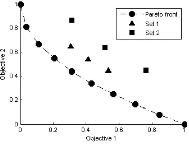
The example in figure 5 illustrates the trade-off between proximity and diversity. Set 2 has a more diverse population of solutions in comparison to Set 1; however Set 1 is closer in proximity to the Pareto-optimal front than Set 2. In this case, the better diversity offered by Set 2 is not as valuable as the proximity offered by Set 1.
Figure 5. An illustration of the trade-off between proximity and diversity to the Pareto-optimal front of an objective function.
C. Methods of Diversity Preservation
1) Niching: One of the earliest forms of diversity preserva-tion in MOEAs is to usenichingto maintain the diversity in the Pareto-optimal set. This was first proposed by De Jong [28] to combat the problems of population drift in multi-modal single objective EAs and aims to maintain multiple niches in the
population by modelling competition amongst individuals in the same niche for limited resources. This results in a selection pressure towards less crowded areas of the search space. In the
crowding factorapproach to niche formation [28], the solution
from a sample of the parent population which is most similar to the child solution is replaced in the current generation. Many of the early generation of Pareto-based MOEAs used some kind of niching based diversity preservation mechanism such as fitness sharing in objective space.
[image:5.612.347.534.325.467.2] [image:5.612.83.273.364.506.2] [image:5.612.82.273.553.693.2]its selection process towards an approximation set with uni-formly spread out solutions. Associated with each individual in a population is two algorithm specific properties: a non-domination rank, in which solutions are ranked by the number of solutions they are dominated by, found using the fast non-dominated sorting approach; and a local crowding distance, which is an estimation of the density of solutions surrounding a particular solution in the population [22], [29]. Between two solutions with different non-domination ranks, the solution with the lower rank is given preference. However, if both solutions are of the same domination rank, then the solution which is located in a region with the least number of solutions is given preference.
3) Bounded Pareto Archiving: Bounded Pareto archiving
(as in the adaptive grid archiving strategy used in both PAES and the CMA-PAES algorithm introduced in this paper) is a simple yet powerful diversity preservation scheme which uses an adaptive grid to keep track of the density of solutions within the search space [6]. To achieve this a grid with a pre-set number of divisions is used to divide the search space, and when a solution is generated its grid location is identified and associated with it. Each grid location is considered to contain its own population, and information on how many
solutions in the archive are located in a certain grid location is available during the optimisation process. When the archive has reached capacity and a candidate solution is to be archived, the information tracked by the adaptive grid algorithm is used to replace a solution in a population containing the highest number of solutions, on the condition that the candidate solutions own grid location does not contain that number. When a candidate solution is non-dominated in regards to the current solution and the archive, the grid information is used to select the solution from the grid location with the smaller population size.
IV. METHODOLOGY
A. CMA-PAES
The purpose for the design and development of CMA-PAES was to arrive at a MOEA benefiting from both the diversity preservation features of AGA and the fast convergence and adaptation of the CMA-ES. A PAES inspired structure was selected as the base framework - due to the simplicity of the algorithm - and thus extending the algorithm with enhance-ments is an intuitive task. The CMA scheme for maintaining a covariance matrix and mutating solutions was inserted in the appropriate areas of the framework, resulting in a modular algorithm which directs the flow of operations through the pre-eminent features of its contributing algorithms.
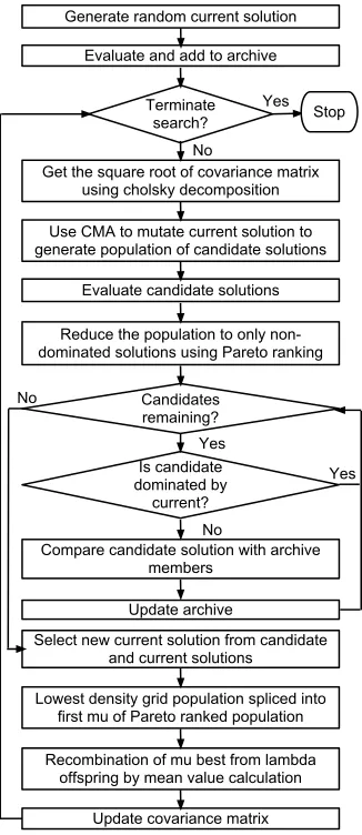
CMA-PAES begins by initializing the algorithm variables and parameters including: the number of grid divisions used in the AGA; the archive for storing non-dominated solutions; the parent vector Y; and the covariance matrix. An initial current solution is then generated at random, evaluated and then the first to be added to the archive. The generational loop then begins, the square root of the covariance matrix is resolved using Cholsky decomposition, and then λ candidate
solutions are generated using copies of the current solution and the CMA-ES procedure for mutation before being evaluated. The archive is then merged with the newly generated offspring and subjected to Pareto ranking, this assigns a rank of zero to all non-dominated solutions, and a rank reflecting the number of solutions that dominate inferior solutions. These population is then purged of inferior solutions so that only non-dominated solutions remain before being fed into the Bounded Pareto Archiving procedure. After the candidate solutions have gone through the archiving procedure and the grid has been adapted to the new solution coverage of objective space, the archive is scanned to identify the grid location with the smallest population, this is considered the lowest density grid population (ldgp) . The solutions from the ldgp are then
spliced onto the end of the first µ−ldgpof the Pareto rank ordered population to be included in the adaptation of the covariance matrix, with the aim to improve the diversity of the next generation by encouraging movement into the least dense area of the grid. After the covariance matrix is updated, the generational loop continues onto its next iteration until the pre-specified maximum number of generations are met. The flow of the algorithm is illustrated in figure 6.
B. ZDT Test Suite
Both CMA-PAES and NSGA-II were tested using the ZDT suite of test functions defined in [30]. The test suite contains six test functions which provide sufficient complexity to compare multi-objective optimisers: ZDT1, ZDT2, ZDT3, ZDT4, ZDT5 and ZDT6, with each function incorporating a feature that is known to cause the EMO process difficulty in convergence to the Pareto-optimal front, and the maintenance of diversity in the approximation set. Each test function has two objectives and is concerned with their minimisation.
A summary of each of the difficult features that each ZDT test function imposes is given in the following:
ZDT1-30 variable problem; convex Pareto-optimal front. ZDT2-30 variable problem; convex Pareto-optimal front. ZDT3-30 variable problem; Pareto-optimal front consists
of non-contiguous convex parts. Discontinuity in the Pareto-optimal front introduced with sine function. ZDT4-10 variable problem; tests the ability to handle
multi-modality with219 local Pareto-optimal fronts.
ZDT6 10 variable problem; solutions non-uniformly dis-tributed along Pareto-optimal front. Low diversity of solutions near the Pareto-optimal front.
ZDT5 was not included in the experiment due to the require-ment for binary represented decision variables. Each algorithm was tested using the parameters specified in section IV-D.
C. Performance Metrics and Randomisation Testing
Candidates remaining?
Generate random current solution
Evaluate and add to archive
Terminate
search? Stop
Use CMA to mutate current solution to generate population of candidate solutions
Evaluate candidate solutions
Is candidate dominated by
current?
Compare candidate solution with archive members
Update archive
Select new current solution from candidate and current solutions
Yes
Yes
No
Reduce the population to only non-dominated solutions using Pareto ranking
Yes No
Get the square root of covariance matrix using cholsky decomposition
No
Recombination of mu best from lambda offspring by mean value calculation
Update covariance matrix Lowest density grid population spliced into
[image:7.612.93.256.54.430.2]first mu of Pareto ranked population
Figure 6. Flow diagram of CMA-PAES, will change this to flow straight and be wider and take up less vertical space
in terms of proximity to the true Pareto-optimal front and the diversity of solutions in the population.
A statistical comparison of the performance of CMA-PAES and NSGA-II was conducted by computing the t-values2 of
the proximity and diversity metrics produced by both the algorithms. Two aspects of the quality of the approximation set produced by the optimiser are used here to characterise the performance of the algorithm: the proximity to the true Pareto-optimal front (measured by the generational distance [31]) and the diversity of the approximation set (measured by the spread [22]).
The significance of these results was then analysed using
randomisation testing. The main advantage of randomisation testing is that it is a non-parametric test and therefore does not require any assumptions to be made about the data [32]. The basic premise is that, if the null hypothesis is true (i.e. that any difference in performance has arisen by chance), then the observed result will appear as a typical value in many random
2The t-value is the difference between the means of the datasets divided
by the standard error.
re-samplings of the data. The randomisation test procedure is outlined below:
1) Compute the t-value of the two datasets. This is the observed result.
2) Randomly reshuffle the data and divide into two sets. Then recompute the t-value.
3) Repeat step 2 a large number of times to obtain the randomised distribution.
4) If the observed result appears a typical value in this randomised distribution, the accept the null hypothesis as true. Otherwise consider the alternative hypothesis (i.e. that one algorithm has outperformed the other). If the observed result appears in the top 5% of the randomised distribution it is said to be “significant at the 5% level”.
In the following experiments, the results of randomisation testing is shown graphically. Figure 7 illustrates a typical ran-domisation test result. The randomised distribution is shown as a histogram and the observed result is shown as an asterisk on thexaxis. An observed result to the left of the histogram
indicates that set A outperforms set B, whilst an observed result to the right indicates the opposite is true (since the smaller the t-value the better the performance of set A). An observed result towards the middle of the histogram indicates that the null hypothesis is true. In the following experiments, set A represents CMA-PAES, and set B represents NSGA-II.
Figure 7. An example randomisation test result (set B outperforms set A)
D. Algorithm Configurations
The algorithms have been configured so they execute both 8000 function evaluations on each problem by ensuring the population size and number of generations for each algorithm are configured correctly. These parameter configurations are presented in table I. NSGA-II generates and evaluates a population of 100 individuals at each of the 80 generations, compared with CMA-PAES which generates and evaluates 400 individuals at each of the 20 generations.
V. RESULTS
[image:7.612.314.564.383.472.2]Figure 8. Randomisation testing results for proximity and diversity performance between NSGA-II and CMA-PAES, illustrated as a histogram.
Table I
PARAMETERS USED FOR TESTINGNSGA-IIANDCMA-PAES,WHEREn IS THE NUMBER OF DECISION VARIABLES.
Parameter NSGA-II CMA-PAES µ/ Population 100 100
λ/ Offspring 100 400
Generations 80 20
Archive Capacity — 100
Grid Divisions — 100
Mutation Rate 1/n —
Crossover Rate 0.9 —
On the test functions ZDT1 to ZDT3, the results indicate that with the algorithm configurations and performance metrics used, CMA-PAES provides better performance in regard to both the proximity of the approximation set to the true Pareto-optimal front, as well as better diversity of solutions within that approximation set. This also verifies that CMA-PAES is capable of converging to convex (or several non-contiguous convex) and non-convex Pareto-optimal fronts in search spaces of up to 30 variables.
The results for the ZDT4 test function shows better proxim-ity to the true Pareto-optimal front for CMA-PAES; however, should a higher number of function evaluations be allowed the CMA-PAES is expected to prematurely converge to a local Pareto-front and get stuck there. This behaviour has been seen in [25] for the MO-CMA-ES algorithm and is a feature of the CMA strategy used for variation. Therefore it is assumed that CMA-PAES on ZDT4 converges to or close to a local Pareto-optimal front, but does it quickly, explaining why on fewer function evaluations CMA-PAES outperforms NSGA-II. If a higher number of function evaluations were allowed it is expected that NSGA-II would consistently outperform the
CMA-PAES on ZDT4.
The results for the ZDT6 test function indicate that CMA-PAES performs better than NSGA-II in both proximity and diversity; however, the difference in proximity is less pro-nounced than in the other test functions used. This also verifies that the CMA-PAES is capable of converging to the Pareto-optimal front whilst maintaining good diversity when there is non-uniformity in the search space, with non-uniformly distributed solutions along the global Pareto-optimal front and reduction in density as proximity to that global front decreases. A comparison with PAES is also presented in table II, where it can be seen that CMA-PAES generally out-performs PAES on all test functions except ZDT 4 and 6. PAES was configured to run for8000generations using the(1 + 1)scheme, with the same AGA parameters as CMA-PAES and a mutation rate of 0.1.
.
Table II
MEAN PROXIMITY AND DIVERSITY PERFORMANCE BETWEENNSGA-II, CMA-PAES (LABELLEDC-PAES)ANDPAES,WHERE BOLD INDICATES
BETTER PERFORMANCE.
Proximity Diversity
NSGA-II C-PAES PAES NSGA-II C-PAES PAES ZDT1 5.5424e-3 2.9595e-6 6.5509e-4 0.54068 0.3196 0.46956
ZDT2 8.0361e-3 2.6856e-6 3.7290e-4 0.63053 0.3484 0.5163
ZDT3 6.5881e-3 2.9433e-5 6.0431e-4 0.73752 0.52584 0.74639
ZDT4 5.2814e+1 1.8062e+1 0.22426 0.93150 0.97824 0.84992
ZDT6 2.4718e-2 1.5756e-2 7.2758e-3 1.1212 0.5923 0.7325
VI. CONCLUSIONS
close to or on the true Pareto-optimal front as well as returning a diverse set of solutions in regards to points in objective space. These observations held in the comparison with NSGA-II on equal function evaluations, however, in this paper, no serious attempt was made to find the optimal parameter settings for CMA-PAES. As previously mentioned CMA-PAES and other CMA driven MOEAs fail to perform adequately on ZDT4, further work is to be put into identifying a method for preventing CMA-PAES to be deceived into prematurely converging to locally Pareto-optimal fronts. There is potential in treating a small portion of the population to additional methods of mutation (e.g. Gaussian mutation) to encourage exploration of the search space independent of the CMA mutation scheme.
Further work on the CMA-PAES is planned to improve the pertinence of its final approximation set by using preference articulation techniques such as those used in the Indicator Based Evolutionary Algorithm (IBEA) [33], allowing focus and encouragement towards a desired ROI during the EMO process. A review and discussion of popular methods of incorporating preference articulation into an EMO can be found in [34]. Further performance analysis is also required to investigate the performance of CMA-PAES on problems of greater than two objectives, such as the test instances described in CEC 2009 [35], as well as a comparison between CMA-PAES and other MOEAs using CMA such as the MO-CMA-ES variants.
REFERENCES
[1] F. Y. Edgeworth,Mathematical psychics: An essay on the application of mathematics to the moral sciences. CK Paul, 1881, no. 10. [2] C. Coello, “Theoretical and numerical Constraint-Handling techniques
used with evolutionary algorithms: A survey of the state of the art,” 2002.
[3] K. Deb, “Multi-Objective optimization using evolutionary algorithms,” 2001.
[4] R. Purshouse and P. Fleming, “On the evolutionary optimization of many conflicting objectives,”Evolutionary Computation, IEEE Transactions on, vol. 11, no. 6, pp. 770–784, 2007.
[5] N. Hansen and A. Ostermeier, “Adapting arbitrary normal mutation distributions in evolution strategies: The covariance matrix adaptation,” inEvolutionary Computation, 1996., Proceedings of IEEE International Conference on, 1996, pp. 312–317.
[6] J. Knowles and D. Corne, “The pareto archived evolution strategy: a new baseline algorithm for pareto multiobjective optimisation.” IEEE, 1999, pp. 98–105.
[7] C. Darwin, “On the origin of species by means of natural selection, or the preservation of favoured races in the struggle for life,”New York: D. Appleton, 1859.
[8] G. Mendel, “Experiments in plant hybridization (1865),” inRead at the meetings of February 8th, and March 8th, 1865.
[9] S. Wright, “The roles of mutation, inbreeding, crossbreeding, and selection in evolution,” in Proc of the 6th International Congress of Genetics, vol. 1, 1932, pp. 356–366.
[10] J. H. Holland,Adaptation in natural and artificial systems. University of Michigan Press, 1975.
[11] D. E. Goldberg,Genetic Algorithms in Search, Optimization and Ma-chine Learning, 1st ed. Boston, MA, USA: Addison-Wesley Longman Publishing Co., Inc., 1989.
[12] I. Rechenberg, “Cybernetic solution path of an experimental Prob-lem",(Royal aircraft establishment translation no. 1122, BF toms, trans.),” Farnsborough Hants: Ministery of Aviation, Royal Aircraft Establishment, 1965.
[13] H. P. Schwefel, “Projekt MHD-Staustrahlrohr: experimentelle optimier-ung einer zweiphasenduse, teil i,” Technischer Bericht 11.034/68, 35, AEG Forschungsinstitut, Berlin, Germany, Tech. Rep., 1968.
[14] N. Hansen, S. D. MÃijller, and P. Koumoutsakos, “Reducing the time complexity of the derandomized evolution strategy with covariance matrix adaptation (CMA-ES),”Evolutionary Computation, vol. 11, no. 1, pp. 1–18, 2003.
[15] A. Auger and N. Hansen, “A restart CMA evolution strategy with increasing population size,” in Evolutionary Computation, 2005. The 2005 IEEE Congress on, vol. 2, 2005, pp. 1769–1776.
[16] ——, “Performance evaluation of an advanced local search evolutionary algorithm,” inEvolutionary Computation, 2005. The 2005 IEEE Con-gress on, vol. 2, 2005, pp. 1777–1784.
[17] W. Jakob, M. Gorges-Schleuter, and C. Blume, “Application of genetic algorithms to task planning and learning,”Parallel problem solving from nature, vol. 2, pp. 291–300, 1992.
[18] C. Coello, “A comprehensive survey of evolutionary-based multiob-jective optimization techniques,”Knowledge and Information systems, vol. 1, no. 3, pp. 269–308, 1999.
[19] ——, “Evolutionary multi-objective optimization: a historical view of the field,”Computational Intelligence Magazine, IEEE, vol. 1, no. 1, pp. 28–36, 2006.
[20] J. Knowles and D. Corne, “Approximating the nondominated front using the pareto archived evolution strategy,”Evolutionary computation, vol. 8, no. 2, pp. 149–172, 2000.
[21] D. Corne, J. Knowles, and M. Oates, “The pareto envelope-based selection algorithm for multiobjective optimization,” inParallel Problem Solving from Nature PPSN VI, 2000, pp. 839–848.
[22] K. Deb, S. Agrawal, A. Pratap, and T. Meyarivan, “A fast elitist non-dominated sorting genetic algorithm for multi-objective optimization: NSGA-II,”Lecture notes in computer science, vol. 1917, pp. 849–858, 2000.
[23] C. Igel, N. Hansen, and S. Roth, “Covariance matrix adaptation for multi-objective optimization,”Evolutionary Computation, vol. 15, no. 1, pp. 1–28, 2007.
[24] E. Zitzler and L. Thiele,An evolutionary algorithm for multiobjective optimization: The strength pareto approach. Citeseer, 1998. [25] T. Voss, N. Hansen, and C. Igel, “Improved step size adaptation for
the MO-CMA-ES,” in Proceedings of the 12th annual conference on Genetic and evolutionary computation, 2010, pp. 487–494.
[26] Q. Zhang and H. Li, “MOEA/D: a multiobjective evolutionary algorithm based on decomposition,”Evolutionary Computation, IEEE Transactions on, vol. 11, no. 6, pp. 712–731, 2007.
[27] P. A. N. Bosman and D. Thierens, “The balance between proximity and diversity in multiobjective evolutionary algorithms,” Evolutionary Computation, IEEE Transactions on, vol. 7, no. 2, pp. 174–188, 2003. [28] K. A. De Jong, “Analysis of the behavior of a class of genetic adaptive
systems,” 1975.
[29] K. Deb, A. Pratap, S. Agarwal, and T. Meyarivan, “A fast and elit-ist multiobjective genetic algorithm: NSGA-II,”IEEE transactions on evolutionary computation, vol. 6, no. 2, pp. 182–197, 2002.
[30] E. Zitzler, K. Deb, and L. Thiele, “Comparison of multiobjective evolutionary algorithms: Empirical results,”Evolutionary Computation, vol. 8, no. 2, pp. 173–195, Jun. 2000.
[31] D. A. Van Veldhuizen, “Multiobjective evolutionary algorithms: classi-fications, analyses, and new innovations,” DTIC Document, Tech. Rep., 1999.
[32] B. F. J. Manly,Randomization and Monte Carlo methods in biology. London; New York: Chapman and Hall, 1991.
[33] E. Zitzler and S. Kunzli, “Indicator-based selection in multiobjective search,” in Parallel Problem Solving from Nature - PPSN VIII, ser. Lecture Notes in Computer Science. Springer Berlin / Heidelberg, 2004, vol. 3242, pp. 832–842.
[34] C. Coello, “Handling preferences in evolutionary multiobjective optim-ization: a survey,” vol. 1. IEEE, 2000, pp. 30–37.