Edgeworth Approximation of a Finite Sample Distribution
for an AR(1) Model with Measurement Error
Shuichi Nagata
Department of Mathematical Sciences, Kwansei Gakuin University, Sanda, Japan Email: [email protected]
Received July 25, 2012; revised August 27, 2012; accepted September 9, 2012
ABSTRACT
In this paper, we consider the finite sample property of the ordinary least squares (OLS) estimator for an AR(1) model with measurement error. We present the Edgeworth approximation for a finite distribution of OLS up to O(T1 2). We introduce an instrumental variable estimator that is consistent in the presence of measurement error. Finally, a simula- tion study is conducted to assess the theoretical results and to compare the finite sample performances of these estima- tors.
Keywords: Edgeworth Expansion; OLS; Measurement Error; Instrumental Variables Estimator
1. Introduction
The Ordinary Least Squares (OLS) estimator for the AR(1) model is one of the most general estimators in economet- rics, and a number of studies considering the properties of the OLS estimator under certain conditions have been conducted by several authors. For example, it is well known that the OLS estimator for the AR(1) model has a non-negligible bias when the sample size T is not large. This problem is known as the small sample problem ([1, 2]).
Another problem of the OLS estimator is that the ob- servation data are sometimes contaminated by noise, which also affects the estimation result. In this case, the OLS estimator in the AR(1) model is not consistent. This problem is commonly known as the measurement error problem. Following [3] that summarized the early results on this topic, numerous articles have been published on this topic. For example, with respect to time series analy- sis, some estimators in an AR model with measurement errors in [4] and statistical a test for the existence of noise is proposed in [5].
In this paper, we deal with these two important prob- lems simultaneously. In particular, we consider the OLS estimation when the sample size T is not large, and when an measurement error is present but ignored. To evaluate the effect of a small sample size and ignoring measure- ment error, we derive finite sample properties of the OLS estimator with noise using the Edgeworth expansion, which is a traditional technique in econometrics to ap- proximate a finite sample distribution. For example, the OLS estimator was studied in [6] for pure AR(1), in [7]
for AR(1) with an unknown mean, and in [8] for AR(1) with exogenous variables. Following these studies, we apply the algorithm proposed in [9] to calculate the Edgeworth coefficients.
In our setting, some problems are the result of noise, which make calculation difficult. First, if data are af- fected by noise, it is difficult to obtain variables that are related to the autocovariance function of the observation process. To obtain these variables, we use the result in [10], which shows that an AR(1) process together with noise can be represented by an ARMA(1, 1) process. Second, the OLS estimator is inconsistent with noise, and it is impossible to apply the formula in [9] in this case; hence we use a corrected error function that follows [8] and [11] to avoid this problem.
In the simulation section, we also consider a instru- mental variable (IV) estimation, which is the consistent estimation in our setting. We compare the finite sample performances of the OLS estimator with those of our proposed IV estimator using simulations.
This paper is organized as follows. In the next section, we provide our setting and the main result for the Edge- worth approximation of the OLS estimator up to O(T1 2). In Section 3, we examine a Monte Carlo simulation and graphical comparison. Finally, Section 4 concludes this paper.
2. Setup and Main Results
2 2
. 0, ,
. . . 0, ,
u
d N
i i d N
1
, ~ . .
, ~
t t t t t t t t
y x u u i i
x x
(1)
where only yt is observable, xt is a stationary AR(1)
process with 1
0,1, ,
t T
and ut is the measurement error or
noise. For a given sample period , the OLS estimate can be written as follows:
1 2
ˆ y C y,
y C y
0, , T
(2)
where y y y ,
1 2
1
0 0 0
2
1 0
1 0 0 0
0 1 2
1 0
0 0
2 0 0
1
0 0 0
2 C C 0 0 0 0 .
0 1 0
0 0 2
The result of this paper relies on the following well known result given in [10]. If xt is an AR(1) process with
AR parameter β, and ut is white noise with constant
variance , then yt follows an ARMA(1, 1) process,
which is given by the following equations:
1L
yt
1 L
t,
2
~ . . . 0, ,
t i i d N
2
(3) where L is the lag operator. The parameters and γ (the MA parameter) can be related to β, 2
, and 2
as follows:
2 1 1 4
, , 2 q q
2 2 u where 2 2 2 2u u 1 q .
Then, we obtain the following theorem.
Theorem 1. The finite sample distribution of the OLS estimator up to O(T1 2) is given by
2 6 Q Qw , 14 3 2 6 1 2 6 1
ˆ
3
T d
p w
i w P
I w P P P
T P P P
where i w
1 2π
12exp
w2 2 ,
I
w wi t t
d
1, ,6
i
P i
.
1 2 4 2 6 1 2
P P P
P1
r
1 r
ω, and Q are as follows:
, 2
2 1 2
P r r
,
5 2 4 4 3 3 4 3 2 3 3
2 3 2 4 3
2 2
4 4
P r r r r r
r r r r r
,
4 2 3 3 2 2 2 4 2 2
4 3 2 2 3 2
P r r r r r r
,
3 4 3 3 2 3 3 2 4
5
7 5 5 2 4 4 3 6 5
6 3 5 4 9 4 3 10 5 4 5 2 6 3 7 4 8 5 7 6
6 5 6 7 7 4 8 5 6
7 8 3
3 62 6 3 8 32
6 16 24 12 26 16
20 32 12 3 84
8 62 4 4 4
32 20 26 24 32
8 2 3 ,
P r r r r r
r r r r r r
r r r r r
r r r r r
r r r r r
r r ,
3 2 4 5 5 2
6
2 2 4 2 3 3
6 5 2 4 3 4 3
6 3 5 4 3 6 3 5 4
10 3 6
3 4 3 9
4 4 9
2 6 4 3
P r r r r r
r r r r
r r r r
r r r r r
3 2 2
5 2 5 2 6 4 1 3 2 12 4 1
Q P PP P P P P P P P
,
.
Proof. The proof is given in Appendix.
Here, we also examine the IV estimator, which is de- fined as follows:
2 2 1 2 T i i i T i i i y y y y
. (4)
The IV estimator is consistent in the presence of the noise. It is easy to show that the asymptotic variance of the IV estimator is
12
22 1
. When there is no noise, the asymptotic variance of the OLS estimator is 1 –β2.
Therefore, the OLS estimator is more efficient than the IV estimator in the absence of noise.
3. Simulation and Graphical Comparison
In this section, we examine the finite sample property of the OLS estimator, and evaluate the approximate distri- bution generated in Section 2 by Monte Carlo simulation.Data were simulated from Equation (1) with . Therefore, the noise-to-signal ratio 2 2 2
throughout this section. In addition to the OLS estimator, we also compute the IV estimator defined in the previous section. The number of replications was 20,000. We computed the mean (Mean) and the root mean squared error (RMSE) for each estimator. The simulation results are summarized in Tables 1-3.
Table 3. Simulation results (ρ = 0.7). Table 1. Simulation results (ρ = 0.2).
β= 0.4 β= 0.8
Mean RMSE Mean RMSE
T OLS IV OLS IV OLS IV OLS IV
20 0.31 0.91 0.24 68.73 0.68 0.71 0.23 1.68
40 0.33 0.58 0.17 45.50 0.71 0.75 0.16 0.22
100 0.34 0.20 0.12 23.74 0.73 0.78 0.11 0.10
500 0.34 0.40 0.07 0.13 0.74 0.80 0.07 0.04
800 0.34 0.40 0.07 0.10 0.74 0.80 0.06 0.03
β = 0.4 β = 0.8
Mean RMSE Mean RMSE
T OLS IV OLS IV OLS IV OLS IV
20 0.23 0.62 0.28 109.62 0.56 0.59 0.32 12.6 40 0.24 0.99 0.22 72.55 0.60 0.77 0.26 2.89 100 0.25 0.37 0.18 4.39 0.62 0.78 0.20 0.12 500 0.25 0.40 0.16 0.18 0.64 0.80 0.17 0.05 800 0.25 0.40 0.15 0.14 0.64 0.80 0.17 0.04
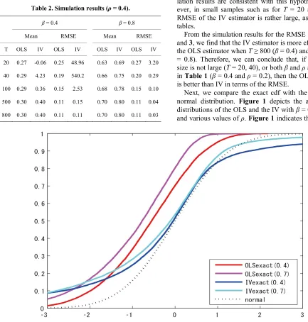
[image:3.595.59.492.268.722.2]the larger the noise variance, the larger will be the bias. On the other hand, as the IV estimator is a consistent estimator, IV may converge to the true value. The simu- lation results are consistent with this hypothesis. How- ever, in small samples such as for T = 20 and 40, the RMSE of the IV estimator is rather large, as seen in all tables.
Table 2. Simulation results (ρ = 0.4).
β= 0.4 β= 0.8
Mean RMSE Mean RMSE
T OLS IV OLS IV OLS IV OLS IV
20 0.27 -0.06 0.25 48.96 0.63 0.69 0.27 3.20
40 0.29 4.23 0.19 540.2 0.66 0.75 0.20 0.29
100 0.29 0.36 0.15 2.53 0.68 0.78 0.15 0.10
500 0.30 0.40 0.11 0.15 0.70 0.80 0.11 0.04
800 0.30 0.40 0.11 0.11 0.70 0.80 0.11 0.03
From the simulation results for the RMSE in Tables 2
and 3, we find that the IV estimator is more efficient than the OLS estimator when T≥ 800 (β = 0.4) and T≥ 100 (β = 0.8). Therefore, we can conclude that, if the sample size is not large (T = 20, 40), or both βandρ are small as in Table 1 (β = 0.4andρ = 0.2), then the OLS estimator is better than IV in terms of the RMSE.
Next, we compare the exact cdf with the asymptotic normal distribution. Figure 1 depicts the approximate distributions of the OLS and the IV with β= 0.4, T = 20, and various values ofρ. Figure 1 indicates that the OLS
values have a downward bias. The IV exhibits good be- havior in the central region of the distribution; however, its distribution is fatter in the tails compared to the nor- mal distribution.
Finally, we evaluate the approximate distributions ob- tained in Section 2, and compare them with the exact cdf and asymptotic normal distributions. To enable a com-
[image:4.595.126.465.179.726.2]parison of the shapes of the distributions, the asymptotic bias of the OLS estimator is corrected hereinafter. Fig- ure 2 shows the approximate distributions of the OLS estimator with T = 20, ρ = 0.2, and three different values of β. From this figure, we can observe the same result as those obtained in [6]. Figure 3 depicts the approximate distributions of the OLS withρ = 0.7, where the other pa-
Figure 2. Exact and approximate distributions of OLS.
0.8
rameter values are the same as those for Figure 2. We note that the shapes of the distributions are almost the same, even if the noise ratio ρ is changed. From these figures, the noise variance has only a small effect on the shape of the OLS distribution.
4. Discussion
In this paper, we considered finite sample properties of the OLS estimator for the AR(1) model with measure- ment error. Using the formula in [9], we obtained the Edgeworth expansion for finite sample distributions of the OLS estimator up to O(T1 2).
In the simulation work, we have compared naive OLS estimator with the IV estimator which is a consistent es- timator in the presence of noise. We can confirm that, even if the measurement errors is exist, the OLS estima- tor is more efficient than the IV estimator when the sam- ple size is small such as T = 20 and 40. If the noise- to-signal ratio is not so small (ρ≥ 0.4), the IV estimator is more efficient than the OLS estimator when T≥ 800 (β = 0.4) or T≥ 100 (β = 0.8). From the graph of the nor- malized OLS distributions, we find similar properties to those of the distributions, which correspond to the no noise situation examined by [6]. This result implies that measurement error mainly distorts the OLS distributions for mean and variance; hence we can separately deal with the two problems of small sample size and observation errors.
Recently, the differenced-AR(1) estimator was dis- cussed in [12,13]. Even if the sample size T is relatively small, this estimator has a small bias. To obtain the finite sample distribution and to examine the robustness of such estimators with respect to observation errors, we can apply the technique of this paper, and this will be dealt with in a future study.
5. Acknowledgements
I am grateful to Professor Koichi Maekawa for his guid- ance on this topic and his valuable comments on this paper. I am also grateful to Professor Yasuyoshi Tokutsu for his valuable comments.
REFERENCES
[1] F. H. C. Marriott and J. A. Pope, “Bias in the Estimation
of Autocorrelations,” Biometrika, Vol. 41, No. 3-4, 1954, pp. 390-402. doi:10.2307/2332719
[2] M. G. Kendall, “Note on the Bias in the Estimation of Autocorrelation,” Biometrika, Vol. 41, No. 3-4, 1954, pp. 403-404. doi:10.2307/2332720
[3] W. A. Fuller, “Measurement Error Models,” John Wiley, New York, 1987. doi:10.1002/9780470316665
[4] J. Staudenmayer and P. Buonaccorsi, “Measurement Er- ror in Linear Autoregressive Model,” Journal of the Ameri- can Statistical Association, Vol. 100, No. 471. 2005, pp. 841-851. doi:10.1198/016214504000001871
[5] K. Tanaka, “A Unified Approach to the Measurement Error Problem in Time Series Models,” Econometric The- ory, Vol. 18, No. 2, 2002, pp. 278-296.
doi: 10.1017/S026646660218203X
[6] P. C. B. Phillips, “Approximations to Some Sample Dis- tributions Associated with a First Order Stochastic Dif- ference Equation,” Econometrica, Vol. 45, No. 2, 1977, pp. 463-485. doi.org/10.2307/1911222
[7] K. Tanaka, “Asymptotic Expansions Associated with the AR(1) Model with Unknown Mean,” Econometrica, Vol. 51, No. 4, 1983, pp. 1221-1231. doi:10.2307/1912060 [8] K. Maekawa “An Approximation to the Distribution of
the Least Squares Estimator in an Autoregressive Model with Exogenous Variables,” Econometrica, Vol. 51, No.1, 1983, pp. 229-238. doi:10.2307/1912258
[9] J. D. Sargan, “Econometric Estimators and the Edgeworth Expansions,” Econometrica, Vol. 44, No. 3, 1976, pp. 421-448. doi:10.2307/1913972
[10] C. W. J. Granger and M. J. Morris, “Time Series Model- ing and Interpretation,” Journal of the Royal Statistical Society A, Vol. 139, No. 2, 1976, pp. 246-257.
doi:10.2307/2345178
[11] K. Maekawa, “Edgeworth Expansion for the OLS Esti- mator in a Time Series Regression Model,” Econometric Theory, Vol. 1, No. 2, 1985, pp. 223-239.
doi:10.1017/S0266466600011154
[12] K. Hayakawa, “A Note on Bias in First-Differenced AR(1) Models,” Economics Bulletin, Vol. 3 No. 27, 2006, pp. 1- 10.
Appendix
Proof of Theorem 1
The OLS estimator for β is given by Equation (2). Intro- ducing i
i
, we can write the derivation of the estimation as follows:E y C y
2 2 2 . u T1 1 2
2 2
ˆ y C y y C y
y C y
In addition, we introduce i i i and
. Then, we have the error function as; q y C y T
1, 2
q q q
2
q1 q2
2 2
ˆ u .
q T
In order to develop the Edgeworth expansion, we de-fine a modified function e(q):
2 2 22 2
u 1 2 u u T
2 2
ˆ T q q
e q q T .
It is easy to obtain the cumulant generating function of 1 2
T q is
I
1 1C 2C2
,
1 1 2 2
1log det 2 2 , T T T
where θj = itjand 1 2
2 1 3 4 , , , , .
. The matrices Iand Σ are the identity matrix and the covariance matrix of y, re- spectively.
jk j k jkl j k l j jk k jk jk a aj j
e e e e e
e e e
Edgeworth expansion requires the partial derivatives of e(q) and φ(θ) up to the third order. In the current paper these derivatives are denoted as ej, ejk,ψjk and ψjkl, which
are all evaluated at the origin. Using the tensor summa-tion convensumma-tion, Edgeworth coefficients of Sargan’s formula are obtained by these derivatives as follows:
Although we only show Edgeworth coefficients re-lated to approximations of up to O(T1 2), the original formula of Sargan can approximate up to O(T), see [6].
After many calculations, we finally obtain the Edge-worth coefficients. To save space, we show only the re-sults as follows:
2
21 5 3 2 4 1 1 4
1 6 3 3 7 4
2 2
2 6 1 4 1
4 3 2 4 2
2 2
2 1 4 2
, ,
4
, ,
iP P P P P P P P
P P T P P P P P P
where Piand Q are polynomials defined in Section 2.
The approximation of the OLS estimator up to O(T1 2) is derived in [6] as follows.
20 2 ,
x x x
p T e q x I i c c
(5) where c0 and c2 are
3 3
4 1 1
0 3 3 2 3
1 6 6
2 2 2
i i
c c
T T T
.
Using these results, we obtain the following equations.
1 4 6 1 1
0 2
2 6 1 2 6
3 1
3 2 2
6
3 3
P P P P Q PQ
c c
P P P T P P P T