A New Stochastic Restricted Liu Estimator for the Logistic Regression Model

http://www.scirp.org/journal/ojs ISSN Online: 2161-7198

ISSN Print: 2161-718X

DOI: 10.4236/ojs.2018.81003 Feb 1, 2018 25 Open Journal of Statistics

A New Stochastic Restricted Liu Estimator for

the Logistic Regression Model

Weibing Zuo, Yingli Li

College of Mathematics and Statistics, North China University of Water Resources and Electric Power, Zhengzhou, China

Abstract

In order to overcome the well-known multicollinearity problem, we propose a new Stochastic Restricted Liu Estimator in logistic regression model. In the mean square error matrix sense, the new estimation is compared with the Maximum Likelihood Estimation, Liu Estimator Stochastic Restricted Maxi-mum Likelihood Estimator etc. Finally, a numerical example and a Monte Carlo simulation are given to explain some of the theoretical results.

Keywords

Multicollinearity, Liu Estimator, Stochastic Restricted Liu Estimator, Scalar Mean Squared Error Matrix

1. Introduction

Consider the following multiple logistic regression model is

, 1, , ,

i i i

y =π ε+ i=  n (1.1) which follows Bernoulli distribution with parameter πi as

( )

( )

exp

, 1 exp

i i

i

x

x

β π

β

′ =

′

+ (1.2)

where

β

is a

(

p+ ×1

)

1 vector of coefficients and x_i is the ith row of X, which is an n×

(

p+1

)

data matrix with P explanatory variables, εi is inde-pendent with mean zero and variance π_i

(

1−π_i

)

of the response y_i. The maximum likelihood method is the most commonly used method of estimating parameters and the Maximum Likelihood Estimator (MLE) is defined as

1 MLE

ˆ _{C X WZˆ ,}

β ₌ − _′ (1.3)

where _{C=X WX′}ˆ _; ˆ _ˆ

(

_{1 ˆ}

)

i i

W =diag_π −π _ and Z is the column vector with ith How to cite this paper: Zuo, W.B. and Li,

Y.L. (2018) A New Stochastic Restricted Liu Estimator for the Logistic Regression Mod-el. Open Journal of Statistics, 8, 25-37.

https://doi.org/10.4236/ojs.2018.81003

Received: November 28, 2017 Accepted: January 29, 2018 Published: February 1, 2018

Copyright © 2018 by authors and Scientific Research Publishing Inc. This work is licensed under the Creative Commons Attribution International License (CC BY 4.0).

http://creativecommons.org/licenses/by/4.0/

DOI: 10.4236/ojs.2018.81003 26 Open Journal of Statistics element equals log

( )

ˆ

₍

ˆ

₎

ˆ 1 ˆ

i i i

i i

y π

π

π π

− +

− , which is an asymptotically unbiased

esti-mate of

β

. The covariance matrix of ˆ

MLE

β is

( ) (

)

1

1

ˆ ˆ _,

MLE

Cov

β

= X WX′ − =C− (1.4)

Multicollinearity inflates the variance of the Maximum Likelihood Estimator (MLE) in the logistic regression. Therefore, MLE is no longer the best estimate of parameter in the logistic regression model.

To overcome the problem of multicollinearity in the logistic regression, many scholars conducted a lot of research. Schaffer et al. (1984) [1] proposed Ridge Logistic Regression (RLR). Aguilera et al. (2006) [2] proposed Principal Com-ponent Logistic Estimator (PCLE). Nja et al. (2013) [3] proposed Modified Lo-gistic Ridge Regression Estimator (MLRE). Inan and Erdogan (2013) [4] pro-posed Liu-type estimator (LLE).

Some scholars also improve estimation by limiting unknown parameters in the model which may be exact or stochastic. Where additional linear restriction on parameter vector is assumed to hold, Duffy and Santer (1989) [5] proposed Restricted Maximum Likelihood Estimator (RMLE), Siray et al. (2014) [6] pro-posed Restricted Liu Estimator (RLE), Asar Y et al. (2016) [7] proposed Re-stricted Ridge Estimator. Where additional stochastic linear restriction on para-meter vector is assumed to hold, Nagarajah V, Wijekoon P (2015) [8] proposed Stochastic Restricted Maximum Likelihood Estimator (SRMLE), Varathan N, Wijekoon P (2016) [9] proposed Stochastic Restricted Liu Maximum Likelihood Estimator (SRLMLE), Varathan N, Wijekoon P (2016) [10] proposed Stochastic Restricted Ridge Maximum Likelihood Estimator (SRRMLE).

In this article, we propose a new estimator which is called the Stochastic Re-stricted Liu Estimator (SRLE) when the linear stochastic restrictions are available in addition to the logistic regression model. The article is structured as follows. Model specifications and the new estimators are proposed in Section 2. Section 3 is derived to compare the mean square error matrix (MSEM) of SRLE, MLE etc. Section 4 is a Numerical Example. A Monte Carlo Simulation is used to verify the above theoretical results shown in Section 5.

2. The Proposed Estimators

For the unrestricted model given in Equation (1.1), the LLE proposed by Liu (1993), Urgan and Tez (2008), Mansson et al. (2012) is defined as

ˆ ˆ _,

LLE Zd MLE

β = β (2.1) where 0< <d 1 is a parameter and Z_d=

(

C+I

) (

−1 C+dI

)

. The bias and va-riance matrices of the LLE:

( )

ˆLLE

(

d

)

1,

Bias β = Z −I β =b (2.2)

( )

_ˆ 1 _,

LLE d d

DOI: 10.4236/ojs.2018.81003 27 Open Journal of Statistics In addition to sample model (1.1), let us be given some prior information about

β

in the form of a set of j independent linear stochastic restrictions as follows:

( )

( )

; 0, ,

h=Hβ+v E v = Cov v = Ψ _(2.4) where H is a q×

(

p+1

)

of full rank q≤

(

p+1

)

known elements, h is an

q

×

1

stochastic known vector and v is an

q

×

1

random vector of disturbances with dispersion matrix Ψ _{and mean 0, and} Ψ _{is assumed to be known} q q× positive definite matrix. Further, it is assumed that v is stochastically indepen-dent of *

(

)

1, , n

ε

=

ε

_

ε

_{, i.e. E}

( )

ε*_v′ =₀.

For the restricted model specified by Equations (1.1) and (2.4), the SRMLE proposed by Varathan Nagarajah and Pushpakanthie (2015), the SRLMLE pro-posed by Varathan N, Wijekoon P (2016) are denoted as

(

)

1

(

)

1 1

ˆ ˆ ˆ _,

SRMLE MLE C H HC H h H MLE

β

₌

β

₊ − _{′ Ψ +} − _′− ₋

β

(2.5)

ˆ ˆ _,

SRLMLE Zd SRMLE

β = β _(2.6)

respectively, the bias and variance matrices of the SRMLE and SRLMLE:

(

ˆ

)

_0,

SRMLE

Bias β = (2.7)

(

ˆSRLMLE

)

(

d

)

1,

Bias β = Z −I β=b (2.8)

(

)

(

)

1

1 1 1 1

ˆ _,

SRMLE

Cov

β

=C− −C H− ′ Ψ +HC H− ′ − HC− =A (2.9)

and

(

ˆ

)

_,

SRLMLE d d

Cov β =Z AZ (2.10) respectively.

We propose the Mix Maximum Likelihood Estimator (MME) [11] in logistic regression model which through analogy OME [12] in linear model. Defined as follows

(

₁

)

1

(

₁

)

ˆ ˆ _,

MME C H H X Wy H h

β

_{= + ′Ψ}− − _{′ + ′Ψ}−

(2.11)

the bias and variance matrices of the MME:

(

ˆ

)

₀

MME

Bias β = ,

(

)

(

)

1

(

)

1

1 1 1 1 1

ˆ _.

MME

COV

β

= C+H′Ψ−H − =C− −C H− ′ Ψ +− HC H− ′− =B

In this paper, we propose a new estimator which is named Stochastic Re-stricted Liu Estimator. Defined as follows

ˆ ˆ _,

SRLE Zd MME

β = β _(2.12)

the bias and variance matrices of the SRLE:

(

ˆSRLE

) (

ˆSRLE

)

(

d

)

1,

Bias β =E β − =β Z −I β=b (2.13) and

(

ˆ

) (

ˆ

)

_,

SRLE SRLE d d

DOI: 10.4236/ojs.2018.81003 28 Open Journal of Statistics respectively.

Now we will give a theorem and a lemma that will be used in the following paragraphs.

Theorem 2.1. [13] (Rao and Toutenburg, 1995) Let A: n n× such that

0

A> and B≥0. Then A+ ≥B 0.

Lemma 2.1. [14] (Rao et al., 2008) Let the two n n× matrices M>0, N≥0,

then M >N if

(

1

)

max NM 1

λ − _{< .}

3. Mean Square Error Matrix (MSEM) Comparisons of the

Estimators

In this section, we will compare SRLE with MLE, LLE, SRMLE, SRLMLE under the standard of MSEM.

First, the MSEM of _βˆ _{which is an estimator of}

β

_is

( )

ˆ

( )

ˆ

( )

ˆ

( )

ˆ _,

MSEM β =Cov β + Bias β  _{ }Bias β _′ (3.1)

where _Bias

( )

_βˆ _{is the bias vector and Cov}

( )

_βˆ _{is the dispersion matrix. For}

two given estimators βˆ1 and βˆ2, the estimator βˆ2 is considered to be better than βˆ1 in the MSEM criterion, if and only if

(

β βˆ1, ˆ2

)

MSEM

( )

βˆ1 MSEM

( )

βˆ2 0,

∆ = − ≥ _(3.2)

The scalar mean square error matrix (MSE) is defined as

( )

ˆ

(

( )

ˆ

)

_,

MSE

β

=tr MSEM

β

(3.3)

Note that the MSEM criterion is always superior over the scalar MSE criterion, we only consider the MSEM comparisons among the estimators.

3.1. MSEM Comparisons of the MLE and SRLE

In this section, we make the MSEM comparison between the MLE and SRLE. First, the MSEM of MLE and SRLE as

( )

_ˆ 1

,

MLE

MSEM β =C− (3.4) and

(

ˆSRLE

)

d d 1 1,

MSEM β =Z BZ +b b′ (3.5) respectively.

We now compare these two estimates to the criterion of the MSEM

( )

(

)

(

)

1 1 1 1 1 1 1 1 1 ˆ ˆ , MLE SRLRE d d d d MSEM MSEM

C Z BZ b b

C Z BZ b b

M N β β − − ∆ = − ′ = − − ′ = − + = − (3.6)

where 1

1

M =C− and N₁=Z BZ_{d d}+b b_{1 1}′. Obviously, b b1 1′ is non-negative de-finite matrices, 1

C− and Z BZd d are positive definite. Using Theorem 2.1, it is clear that N1 is positive define matrix. By Lemma 2.1, if

(

)

1 max N M1 1 1

DOI: 10.4236/ojs.2018.81003 29 Open Journal of Statistics

where

(

1

)

max N M1 1

λ − _{is the largest eigen value of} 1 1 1

N M− then M1−N1 is positive definite matrix. Based on the above discussions, the following theorem can be proved.

Theorem 3.1. For the restricted linear model specified by Equations (1.1) and (2.4), the SRLE is superior to MLE if and only if

(

1

)

max N M1 1 1

λ − _{< in the MSEM}

sense.

3.2. MSEM Comparisons of the LLE and SRLE

First, the MSEM of LLE as

( )

1

1 1

ˆ _.

LLE d d

MSEM β =Z C Z− +b b′ (3.7) We now compare these two estimates to the criterion of the MSEM

( )

(

)

2

1

2 2 2 2

ˆ ˆ

LLE SRLRE

d d d d

d d

MSEM MSEM

Z C Z Z BZ b b b b Z DZ β β − ∆ = − ′ ′ = − + − = (3.8)

where

(

)

1

1 1 1 1

D=C H− ′ Ψ +− HC H− ′ − HC− . Obviously, Z DZ_{d d} is positive defi-nite. Based on the above discussions, the following theorem can be proved.

Theorem 3.2. For the restricted linear model specified by Equations (1.1) and (2.4), the SRLE is always superior to LLE in the MSEM sense.

3.3. MSEM Comparisons of the SRMLE and SRLE

First, the MSEM of SRMLE as

(

ˆ

)

_.

SRLE

MSEM β =A (3.9) We now compare these two estimates to the criterion of the MSEM

(

)

(

)

(

)

[

]

3

1

1 1 1 1

1 1 1 1 1 1 3 ˆ ˆ SRMLE SRLRE d d d d MSEM MSEM

C C H HC H HC Z BZ b b

C F Z BZ b b

M N β β − − − − − − ∆ = − ′ ′ ′

= − Ψ + − −

′

= − + +

= −

(3.10)

where

(

)

1

1 1 1

F=C H− ′ Ψ +HC H− ′ − HC− and N₃= +F Z BZ_{d d}+b b_{1 1}′. Obviously, 1 1

b b′ is non-negative definite matrices, F and Z BZd d are positive definite. Using Theorem 2.1, it is clear that N3 is positive define matrix. By Lemma 2.1,

if

(

1

)

max N M3 1 1

λ − _{< , where}

(

1

)

max N M3 1

λ − _{is the largest eigen value of} 1 3 1 N M− then M1−N3 is positive definite matrix. Based on the above discussions, the following theorem can be proved.

Theorem 3.3. For the restricted linear model specified by Equations (1.1) and (2.4), the SRLE is superior to SRMLE if and only if

(

1

)

max N M3 1 1

λ − _{< in the}

MSEM sense.

DOI: 10.4236/ojs.2018.81003 30 Open Journal of Statistics

(

ˆSRLMLE

)

d d 1 1.

MSEM β =Z AZ +b b′ (3.11) Now, we consider the following difference

(

)

(

)

4

1 1 1 1

4 4

ˆ ˆ

SRLMLE SRLRE

d d d d

d d d d

MSEM MSEM

Z AZ Z BZ b b b b

Z DZ Z FZ

M N

β β

∆ = −

′ ′ = − + − = −

= −

(3.12)

where M4=Z DZd d and N4 =Z FZd d. Obviously, D, M4 and N4 are pos-itive definite matrices. By Lemma 2.1, if

(

1

)

max N M4 4 1

λ − _{< , where}

(

1

)

max N M4 4

λ −

is the largest eigen value of 1 4 4

N M− then M₄−N₄ is positive definite matrix. Based on the above discussions, the following theorem can be proved.

Theorem 3.4. For the restricted linear model specified by Equations (1.1) and (2.4), the SRLE is superior to SRLMLE if and only if

(

1

)

max N M4 4 1

λ − _{< in the}

MSEM sense.

4. Numerical Example

In this section, we now consider the data set of IRIS from UCI to illustrate our theoretical results.

A binary logistic regression model is set where the dependent variable is as follows. If the plant is Iris-setosa, it is indicated with 0 and if the plant is Iris-versicolor, it is 1. The explanatory variables is as follows. x1: Sepal. Length;

2

x : Petal. Length; and x3: Petal. Width.

The sample consists of the first 80 observations. The correlation matrix can be seen in Table A1 (Appendix A). From Table A1 (Appendix A), it can be seen that the correlations among the regressors are all greater than 0.80 and some of them are close to 0.98 and the condition number is 55.4984 showing that there is a severe multicollinearity problem in this data.

From Table A2 (Appendix A) we can conclude that:

1) With the increase of d, the MSE values of the estimators are decreasing which are LRE, SRRMLE, SRLRE, SRLMLE, SRLE. 2) With the increase of d, the MSE values of the estimators are same which are MLE, SRMLE, MME. 3) The new estimator is always superior to the other estimators.

5. Monte Carlo Simulation

To illustrate the above theoretical results, the Monte Carlo Simulation is used for data Simulation. Following McDonald and Galarneau (1975) [15] and Kibria (2003) [16], the explanatory variables are generated using the following equa-tion.

(

₂

)

1 2

,

1 , 1, 2, , , 1, 2, , ,

ij ij i p

DOI: 10.4236/ojs.2018.81003 31 Open Journal of Statistics In this section, we set ρ to take 0.70, 0.80, 0.99 and n to take 20, 100, 200 for the dependent variable with two and four explanatory variables. The dependent variable yi in (1.1) is obtained from the Bernoulli (πi) distribution where

( )

( )

exp 1 exp i i i x x β π β ′ = ′

+ . The parameter values of β1,,βp are chosen so that 2 1 1 p j j β = =

∑

and β1==βp. Further for the Liu parameter d, some selected values is chosen so that 0≤ ≤d 1. Moreover, for the restriction, we choose

1 1 0 0 1 1 0 0

0 1 1 0 , 2 and 0 1 0 ,

0 0 1 1 1 0 0 1

H h

−

     

     

=_ − _ = −_{ } Ψ =_{ }

 ₋     

     

(5.2)

The simulation is repeated 2000 times by generating new pseudo-random numbers and the simulated MSE values of the estimators are obtained using the following equation

( )

{

( )

}

(

) (

)

* 2000 1 ˆ ˆ ˆ _,

1 _{ˆ ˆ}

2000 n

MSE β Mean tr MSEM β β

β β β β

=

 

= _{ }

′

=

∑

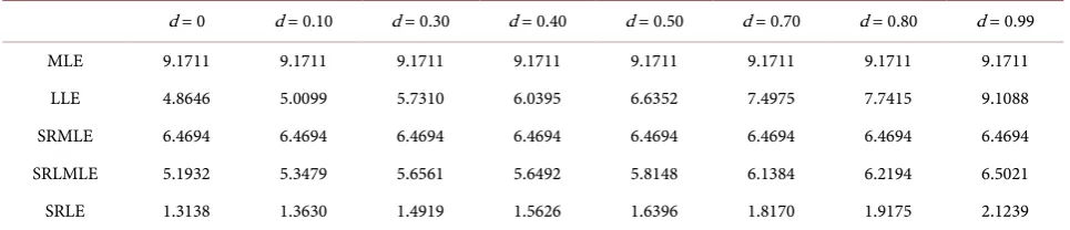
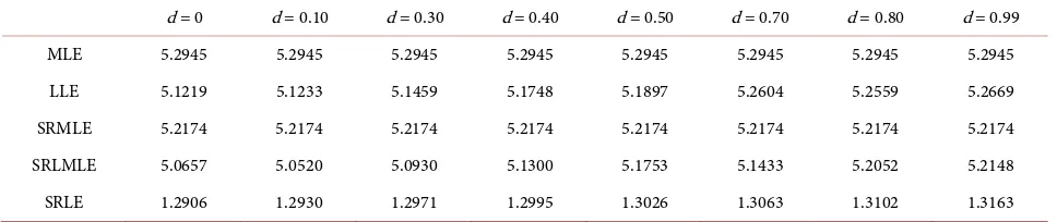
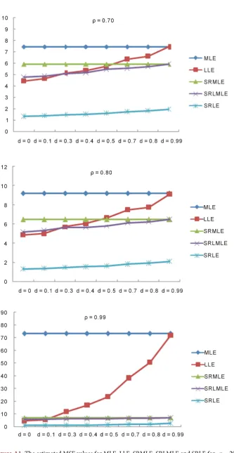
− − (5.3)

The results of the simulation are reported in Tables A3-A9 (Appendix A) and also displayed in Figures A1-A3 (Appendix B).

From Tables A3-A9, Figures A1-A3, we can conclude that:

1) The MSE values of all the estimators are increasing along with the increase of ρ; 2) The MSE values of all the estimators are decreasing along with the in-crease of n; 3) SRLE is always superior to the MLE, LLE, SRMLE, SRLMLE for all

d, n and ρ.

6. Conclusion Remarks

In this paper, we proposed the Stochastic Restricted Liu Estimator (SRLE) for logistic regression model when the linear stochastic restriction was available. In the sense of MSEM, we got the necessary and sufficient condition or sufficient condition that SRLE was superior to MLE, LLE, SRMLE and SRLMLE and Veri-fy its superiority by using Monte Carlo simulation. How to reduce the new esti-mation’s bias is the focus of our next step which guaranteed mean square error does not increase.

Acknowledgements

This work was supported by the Natural Science Foundation of Henan Province of China (No. 152300410112).

References

DOI: 10.4236/ojs.2018.81003 32 Open Journal of Statistics [2] Aguilera, A.M., Escabias, M. and Valderrama, M.J. (2006) Using Principal Compo-nents for Estimating Logistic Regression with High-Dimensional Multicollinear Data. Computational Statistics & Data Analysis, 50, 1905-1924.

https://doi.org/10.1016/j.csda.2005.03.011

[3] Ogoke, U.P., Nduka, E.C. and Nja, M.E. (2013) The Logistic Regression Model with a Modified Weight Function in Survival Analysis. Mathematical Theory & Model-ing, 3, 12-17.

[4] Inan, D. and Erdogan, B.E. (2013) Liu-Type Logistic Estimator. Communication in Statistics—Simulation and Computation, 42, 1578-1586.

https://doi.org/10.1080/03610918.2012.667480

[5] Duffy, D.E. and Santner, T.J. (1989) On the Small Sample Prosperities of Norm-Restricted Maximum Likelihood Estimators for Logistic Regression Mod-els. Communications in Statistics—Theory and Methods, 18, 959-980.

https://doi.org/10.1080/03610928908829944

[6] Şiray, G.Ü., Toker, S. and Kaçiranlar, S. (2014) On the Restricted Liu Estimator in the Logistic Regression Model. Communication in Statistics—Simulation and Computation, 44, 217-232.https://doi.org/10.1080/03610918.2013.771742

[7] Asar, Y., Arashi, M. and Wu, J. (2017) Restricted Ridge Estimator in the Logistic Regression Model. Communication in Statistics—Simulation and Computation, 46.

https://doi.org/10.1080/03610918.2016.1206932

[8] Nagarajah, V. and Wijekoon, P. (2015) Stochastic Restricted Maximum Likelihood Estimator in Logistic Regression Model. Open Journal of Statistics, 5,837-851.

https://doi.org/10.4236/ojs.2015.57082

[9] Varathan, N. and Wijekoon, P. (2016) Logistic Liu Estimator under Stochastic Li-near Restrictions. Statistical Papers, 1-18.

[10] Varathan, N. and Wijekoon, P. (2016) Ridge Estimator in Logistic Regression under Stochastic Linear Restrictions. British Journal of Mathematics & Computer Science, 15, 1-14.https://doi.org/10.9734/BJMCS/2016/24585

[11] Zuo, W.-B. and Li, Y.-L. (2017) Mixed Maximum Likelihood Estimator in Logistic Regression Model. Journal of Henan Institute of Education, 26, 1-6.

[12] Theil, H. and Goldberger, A.S. (1961) On Pure and Mixed Estimation in Econom-ics. International Economic Review, 2, 65-77. https://doi.org/10.2307/2525589

[13] Rao, C.R. and Toutenburg, H. (1995) Linear Models: Least Squares and Alterna-tives. Second Edition, Springer-Verlag, New York.

https://doi.org/10.1007/978-1-4899-0024-1

[14] Rao, C.R., Toutenburg, H., Shalabh and Heumann, C. (2008) Linear Model and Generalizations. Springer, Berlin.

[15] Golam Kibria, B.M. (2003) Performance of Some New Ridge Regression Estimators. Communication in Statistics—Simulation and Computation, 32, 419-435.

https://doi.org/10.1081/SAC-120017499

[16] McDonald, G.C. and Galarneau, D.I. (1975) A Monte Carlo Evaluation of Some Ridge-Type Estimators. Journal of the American Statistical Association, 70, 407-416.

DOI: 10.4236/ojs.2018.81003 33 Open Journal of Statistics

[image:9.595.60.543.108.183.2]

Appendix A

Table A1. The correlation matrix of the dataset.

1

x x2 x3

1

x 1 0.833919 0.811755

2

x 0.833919 1 0.97747

3

[image:9.595.56.543.212.316.2]

x 0.811755 0.97747 1

Table A2. The estimated MSEM values for different d.

k, d = 0 k, d = 0.2 k, d = 0.4 k, d = 0.5 k, d = 0.6 k, d = 0.8 k, d = 0.9 k, d = 0.99 MLE 8.0221e+03 8.0221e+03 8.0221e+03 8.0221e+03 8.0221e+03 8.0221e+03 8.0221e+03 8.0221e+03 LLE 8.0221e+03 220.9556 140.9535 122.7412 110.4983 95.4561 90.5954 87.1297 SRMLE 102.4228 102.4228 102.4228 102.4228 102.4228 102.4228 102.4228 102.4228

SRLMLE 28.0970 33.8486 44.1570 51.0200 59.0222 78.4441 89.8639 101.1157

[image:9.595.56.540.348.450.2]

SRLE 0.7705 0.7863 0.9251 1.0406 1.1869 1.5716 1.8102 2.0511

Table A3. The estimated MSEM values for different d when n=20 and ρ=0.70.

d = 0 d = 0.10 d = 0.30 d = 0.40 d = 0.50 d = 0.70 d = 0.80 d = 0.99

MLE 7.4662 7.4662 7.4662 7.4662 7.4662 7.4662 7.4662 7.4662

LLE 4.4468 4.6588 5.1626 5.3374 5.7376 6.3522 6.6154 7.4366

SRMLE 5.9236 5.9236 5.9236 5.9236 5.9236 5.9236 5.9236 5.9236

SRLMLE 4.7969 4.8832 5.0778 5.1698 5.4686 5.5636 5.7184 5.9218

SRLE 1.3450 1.3954 1.4974 1.5506 1.6109 1.7505 1.8285 1.9793

Table A4. The estimated MSEM values for different d when n=20 and ρ=0.80.

d = 0 d = 0.10 d = 0.30 d = 0.40 d = 0.50 d = 0.70 d = 0.80 d = 0.99

MLE 9.1711 9.1711 9.1711 9.1711 9.1711 9.1711 9.1711 9.1711

LLE 4.8646 5.0099 5.7310 6.0395 6.6352 7.4975 7.7415 9.1088

SRMLE 6.4694 6.4694 6.4694 6.4694 6.4694 6.4694 6.4694 6.4694

SRLMLE 5.1932 5.3479 5.6561 5.6492 5.8148 6.1384 6.2194 6.5021

SRLE 1.3138 1.3630 1.4919 1.5626 1.6396 1.8170 1.9175 2.1239

Table A5. The estimated MSEM values for different d when n=20 and ρ=0.99.

d = 0 d = 0.10 d = 0.30 d = 0.40 d = 0.50 d = 0.70 d = 0.80 d = 0.99

MLE 73.1647 73.1647 73.1647 73.1647 73.1647 73.1647 73.1647 73.1647

LLE 4.5979 5.5820 11.9735 17.0739 23.5922 38.2869 50.5697 71.6768

SRMLE 7.0724 7.0724 7.0724 7.0724 7.0724 7.0724 7.0724 7.0724

SRLMLE 5.9067 6.0027 6.2015 6.2544 6.4525 6.6168 6.8033 6.9489

[image:9.595.57.540.482.586.2] [image:9.595.56.537.617.729.2]

[image:10.595.56.543.90.193.2]

DOI: 10.4236/ojs.2018.81003 34 Open Journal of Statistics

Table A6. The estimated MSEM values for different d when n=100 and ρ=0.7.

d = 0 d = 0.10 d = 0.30 d = 0.40 d = 0.50 d = 0.70 d = 0.80 d = 0.99

MLE 5.0422 5.0422 5.0422 5.0422 5.0422 5.0422 5.0422 5.0422

LLE 4.7008 4.7702 4.7837 4.8357 4.8493 4.9529 4.9284 5.0390

SRMLE 4.9033 4.9033 4.9033 4.9033 4.9033 4.9033 4.9033 4.9033

SRLMLE 4.6768 4.6892 4.7607 4.7660 4.8208 4.8083 4.8644 4.8972

[image:10.595.56.541.224.325.2]

SRLE 1.3186 1.3234 1.3332 1.3395 1.3465 1.3552 1.3621 1.3726

Table A7. The estimated MSEM values for different d when n=100 and ρ=0.8.

d = 0 d = 0.10 d = 0.30 d = 0.40 d = 0.50 d = 0.70 d = 0.80 d = 0.99

MLE 5.6054 5.6054 5.6054 5.6054 5.6054 5.6054 5.6054 5.6054

LLE 5.1351 5.1538 5.2317 5.2462 5.3589 5.5121 5.5192 5.6019

SRMLE 5.4591 5.4591 5.4591 5.4591 5.4591 5.4591 5.4591 5.4591

SRLMLE 5.1120 5.1369 5.2144 5.2191 5.2741 5.3336 5.3462 5.4271

SRLE 1.3596 1.3687 1.3845 1.3930 1.4041 1.4188 1.4303 1.4466

Table A8. The estimated MSEM values for different d when n=200 and ρ=0.8.

d = 0 d = 0.10 d = 0.30 d = 0.40 d = 0.50 d = 0.70 d = 0.80 d = 0.99

MLE 5.2945 5.2945 5.2945 5.2945 5.2945 5.2945 5.2945 5.2945

LLE 5.1219 5.1233 5.1459 5.1748 5.1897 5.2604 5.2559 5.2669

SRMLE 5.2174 5.2174 5.2174 5.2174 5.2174 5.2174 5.2174 5.2174

SRLMLE 5.0657 5.0520 5.0930 5.1300 5.1753 5.1433 5.2052 5.2148

SRLE 1.2906 1.2930 1.2971 1.2995 1.3026 1.3063 1.3102 1.3163

Table A9. The estimated MSEM values for different d when n=200 and ρ=0.99.

d = 0 d = 0.10 d = 0.30 d = 0.40 d = 0.50 d = 0.70 d = 0.80 d = 0.99

MLE 9.0269 9.0269 9.0269 9.0269 9.0269 9.0269 9.0269 9.0269

LLE 5.2509 5.4181 5.9620 6.2403 6.5520 7.4280 7.8798 9.1243

SRMLE 6.1827 6.1827 6.1827 6.1827 6.1827 6.1827 6.1827 6.1827

SRLMLE 5.9722 5.9833 6.0102 6.0147 6.0688 6.1128 6.1244 6.1267

[image:10.595.57.541.365.467.2] [image:10.595.56.538.498.601.2]

DOI: 10.4236/ojs.2018.81003 35 Open Journal of Statistics

[image:11.595.137.471.71.717.2]

Appendix B

DOI: 10.4236/ojs.2018.81003 36 Open Journal of Statistics

Figure A2. The estimated MSE values for MLE, LLE, SRMLE, SRLMLE and SRLE for 100

[image:12.595.139.462.73.479.2]

[image:13.595.133.473.77.683.2]

DOI: 10.4236/ojs.2018.81003 37 Open Journal of Statistics

Figure A3. The estimated MSE values for MLE, LLE, SRMLE, SRLMLE and SRLE for 200