A MULTI-AGENT BASED COOPERATIVE
1APPROACH TO SCHEDULING AND ROUTING
2Simon Martin1, Djamila Ouelhadj2, Patrick Beullens3,
3
Ender Ozcan4,Angel A. Juan5,Edmund.K.Burke1
4
1Computational Heuristics Operational Research Decision Support (CHORDS) Group,
5
University of Stirling, Department of Mathematics and Computer Science, UK
6
email: [email protected]
7
2Centre of Operational Research and Logistics,
8
University of Portsmouth,Department of Mathematics,UK
9
email: [email protected]
10
3Mathematical Sciences and Southampton Business School and CORMSIS, University of
11
Southampton, SO17 1BJ, United Kingdom
12
email: [email protected]
13
4Automated Scheduling, Optimisation and Planning Research Group,
14
University of Nottingham, Department of Computer Science,UK
15
email: [email protected]
16
5Department of Computer Science and Telecommunication,
17
Open University of Catalonia, Rambla Poblenou, 156 088018 Barcelona, Spain
18
email:[email protected]
19
Abstract 20
values for all the benchmarks tested.
Keywords: combinatorial optimization, multi-agent systems, scheduling,
1
vehicle routing, metaheuristics, cooperative search, reinforcement learning.
2
1. INTRODUCTION 3
Heuristics are rules of thumb for solving specific computationally hard
4
problems. Researchers and practitioners use heuristics when exact methods
5
fail to produce any solutions with a “reasonable” quality in a “reasonable”
6
amount of time. Heuristics often come with a set of parameters, each
requir-7
ing tuning for an improved performance. Moreover, different heuristics can
8
perform well on different problem instances. Hence, there is a growing
num-9
ber of studies on more general methodologies which are applicable to different
10
problem domains for tuning the parameters (L´opez-Ib´anez et al., 2011;
Hut-11
ter et al., 2007; Ries and Beullens, 2015), generating or mixing/controlling
12
heuristics (Burke et al., 2013; Ross, 2014). In this study, we take an
alter-13
native approach and use cooperating agents, where each agent is enabled to
14
take a different approach with different parameter settings.
15
By cooperative search we mean that (meta)heuristics, executed in parallel
16
as agents, have the ability to share information at various points
through-17
out a search. To this end, we propose a modular agent-based framework
18
where the agents cooperate using a direct peer to peer asynchronous
mes-19
sage passing protocol. An island model is used where each agent has its own
20
representation of the search environment. Each agent is autonomous and
21
can execute different metaheuristic/local search combinations with different
22
parameter settings. Cooperation is based on the general strategies of pattern
23
matching and reinforcement learning where the agents share partial solutions
24
to enhance their overall performance.
25
The framework has the following additional characteristics. By using
26
ontologies (see Section 3.2), we are aiming to provide a framework that is
27
flexible enough to be used on more than one type of combinatorial
optimi-28
sation problem with little or no parameter tuning. This is achieved by using
29
our scheduling and routing ontology to translate target problems into an
in-30
ternal format that the agents can use to solve problems. So far, this approach
31
has been applied successfully to Capacitated Vehicle Routing (CVRP),
Per-32
mutation Flow shop Scheduling (PFSP), reported here and Nurse Rostering
33
reported in Martin et al. (2013).
The aim of this study is to develop a modular framework for cooperative
1
search that can be deployed, with little reconfiguration, to more than one type
2
of problem. We also test whether interaction between (meta)heuristics leads
3
to improved performance and if increasing the number of agents improves
4
the overall solution quality.
5
1.1. Cooperative search in OR: literature
6
The interest in cooperative search has risen due to successes in finding
7
novel ways to combine search algorithms. Cooperative search can be
per-8
formed by the exchange of states, solutions, sub-problems, models, or search
9
space characteristics. For a general introduction, see e.g. Clearwater et al.
10
(1992); Hogg and Williams (1993); Toulouse et al. (1999); Blum and Roli
11
(2003); Talbi and Bachelet (2006); Crainic and Toulouse (2008). Several
12
frameworks have been proposed recently, incorporating metaheuristics, as in
13
Talbi and Bachelet (2006); Milano and Roli (2004); Meignan et al. (2008,
14
2010), or hyper-heuristics, as in Ouelhadj and Petrovic (2010). Also, El
Ha-15
chemi et al. (2014) explore a general agent-based framework for solution
16
integration where distributed systems use different heuristics to decompose
17
and then solve a problem.
18
In an effort to find ways to combine different metaheuristics in such a
19
way that they cooperate with each other during their execution, a
num-20
ber of design choices have to be made. According to Crainic and Toulouse
21
(2008) anasynchronous framework in particular could result in an improved
22
search methodology; communication can then either be many-to-many
(di-23
rect), where each metaheuristic communicates with every other, or it can be
24
memory based (indirect), where information is sent to a pool that (other)
25
metaheuristics can make use of as required.
26
Most cooperative search mechanisms in the OR literature deploy
indi-27
rect communication through some central pool or adaptive memory. This
28
can take the form of passing whole, or possibly, partial solutions, to the
29
pool. See Talbi and Bachelet (2006); Milano and Roli (2004); Meignan et al.
30
(2008, 2010); Malek (2010). Aydin and Fogarty (2004b) applied this
ap-31
proach to job shop scheduling. Recently Barbucha (2014) has proposed an
32
agent-based system for Vehicle Routing Problems where agents instantiate
33
different metaheuristics which communicate through a shared pool.
34
Direct communication, instead, is used only in Vallada and Ruiz (2009);
35
Aydin and Fogarty (2004a), where whole solutions are passed from one
pro-36
cess to another in an island model executing a genetic or an evolutionary
simulated annealing algorithm respectively, and in Ouelhadj and Petrovic
1
(2010), where a similar set-up is used for a hyper-heuristic. All three
pa-2
pers addressed the PFSP. Also, this approach is to an extent present in the
3
evolutionary system of Xie and Liu (2009), who investigated the Travelling
4
Salesman Problem. Kouider and Bouzouia (2012) propose a direct
com-5
munication multi agent system for job shop scheduling where each agent is
6
associated with a specific machine in a production facility. Here a problem
7
is decomposed into several sub-problems by a “supervisor agent”. These
8
are passed to “resource agents” for execution and then passed back to the
9
supervisor to build the global solution.
10
Little work has been done on asynchronous direct cooperation where
par-11
tial solutions are rated and their parameters are communicated between
au-12
tonomous agents all working on the total problem. So far, no direct
co-13
operation strategy has been applied to more than one problem domain in
14
combinatorial optimisation. To this end, the agents are truly autonomous
15
and not synchronised. There is a gap in the literature regarding agents
co-16
operating directly and asynchronously where the communication is used for
17
the adaptive selection of moves with parameters.
18
The outline for the rest of the paper is as follows. Section 2 provides
19
formal problem statements for the two case studies. Section 3 describes
20
the proposed modular multi-agent framework for cooperative search, while
21
Section 4 describes how it is implemented. In Section 5 we discuss the
exper-22
imental design. In Section 6 we report the results of the tests where, to the
23
best of our knowledge, for three of the capacitated vehicle routing instances
24
we achieved better results than have been reported in the literature. Finally,
25
Section 7 presents conclusions and suggestions for future work.
26
2. TEST CASE PROBLEMS 27
In this section we offer brief problem descriptions of the case studies
28
applied to the agent-based framework proposed in this paper. We chose these
29
instances as they are representative scheduling and routing problems. The
30
algorithms instantiated by the framework are state-of-art implementations
31
(Juan et al., 2014, 2013, 2010a,b). These are all examples of Simheuristics
32
(Juan et al., 2015). This makes them a good fit with the partial solutions
33
identified by the system.
2.1. Permutation flow-shop Scheduling Problem
1
Given is a set of n jobs, J = {1, ..., n}, available at a given time 0, and
2
each to be processed on each of a set of m machines in the same order,
3
M = {1, ..., m}. A job j ∈ J requires a fixed but job-specific non-negative
4
processing time pj,i on each machinei∈M. The objective of the PFSP is to
5
minimise themakespan. That is, to minimise the completion time of the last
6
job on the last machine Cmax (Pinedo, 2002). A feasible schedule is hence
7
uniquely represented by a permutation of the jobs. There are n! possible
8
permutations and the problem is NP-complete (Garey et al., 1976).
9
A solution can hence be represented, uniquely, by a permutation S =
10
(σ1, ..., σj, ...σn), where σj ∈ J indicates the job in the jth position. The
11
completion time Cσj,i of job σj on machine i can be calculated using the
12
following formulae:
13
Cσ1,1 =pσ1,1 (1)
Cσ1,i=Cσ1,i−1+pσ1,i, where i= 2, ..., m (2) Cσj,i=max(Cσj,i−1, Cσj−1,i) +pσj,i,
wherei= 2, ..., m, and j = 2, ..., n (3)
Cmax =Cσn,m (4)
2.2. The Capacitated Vehicle Routing Problem
14
The Capacitated Vehicle Routing Problem (Dantzig and Ramser, 1959)
15
can be defined in the following graph theoretic notation. Let G(V, E) be an
16
undirected complete graph where V ={v0, v1, v2, ...vn} is the vertex set and
17
where vertices E is a set of edges.
18
Let the set vi where i = {1, ...n} represent the customers who are
ex-19
pecting to be serviced with deliveries and let v0 be the service depot. Also
20
associated with each vertex vj is a non-negative demand dj. This value is
21
given each time a delivery is made. For the depot v0 there is a zero demand
22
d0.
23
The set E represents the set of roads that connect the customers to each
24
other and the depot. Thus each edge e ∈ E is defined as a pair of vertices
25
(vi, vj). Associated with each edge is a costci,j of the route between the two
26
vertices.
27
Finally there is also a set of unlimited trucks each with same loading
28
capacity. The aim is to service all the customers visiting them once only and
29
using as few trucks as possible. In any potential delivery round a customer’s
demand has to be taken into account. The total demands of customers on
1
the round must not exceed the capacity of the vehicle. This means that it is
2
normally not possible to visit all customers with one truck. As a consequence
3
each delivery round for a truck is called a route.
4
The goal of the CVRP problem is to minimise the overall travelling
dis-5
tance to service all customers with varying demand using a given number of
6
trucks, each with the same fixed capacity.
7
This problem was proved to be NP-Hard by Garey and Johnson (1979).
8
2.3. Benchmark instances
9
We used the following benchmark instances for testing the experiments
10
described in Section 5. For PFSP, we selected 12 benchmark problems
11
from Taillard (1993). Each Taillard PFSP benchmark instance is labelled
12
as taiX j m, where X is the instance number and (j, m), wherej indicates
13
the number of jobs, and mthe number of machines. In order to facilitate our
14
analysis, we selected 12 of the harder instances two from the (50,20) pool,
15
two from the (100,20) pool and then three from the (200,10) and (200,20)
16
pools and finally three from the (500,20) pool of instances for which an
op-17
timal solution is not known. For CVRP, we tested 12 problems from the
18
benchmarks of Augerat et al. (1995). Each instance of this benchmark is
19
denoted as A−nM −kL, where M and L indicate the number of delivery
20
points including the depot and the target number of routes, respectively.
21
3. AGENT-BASED FRAMEWORK 22
3.1. Framework architecture and operation
23
We describe a general agent-based distributed framework where each
24
agent implements a different metaheuristic/local search combination. An
25
agent continuously adapts itself during the search process using a
cooper-26
ation protocol based on the retention partial solutions deemed as possible
27
constituents of future good solutions. These are shared with the other agents.
28
The framework makes use of two types of agent: launcher and
meta-29
heuristic agents.
30
• The launcher agent is responsible for queueing the problem instances to
31
be solved for a given domain, configuring the metaheuristic agents,
suc-32
cessively passing a given problem instance to the metaheuristic agents
33
and gathering the solutions from the metaheuristic agents. To achieve
this it converts domain specific problem instances into the agent
mes-1
saging protocol using an ontology for scheduling and routing (see
Sec-2
tion 3.2). However the launcher agent plays no actual part in the search,
3
its job is to prepare and schedule problems to be solved by the other
4
agents.
5
• A metaheuristic agent executes one of the metaheuristic/local search
6
heuristic combinations that are available. These combinations and their
7
parameter settings are all defined on launching. In this way each agent
8
is able to conduct searches using different combinations and parameter
9
settings from the other agents employed in the search. Each
meta-10
heuristic agent conducts its search using the messaging structure
de-11
fined in the ontology for scheduling and routing and uses no problem
12
specific data and as such is generic.
13
A search proceeds with the launcher reading a number of problem
in-14
stances into memory. It converts them into objects that can be defined by
15
the Ontology for scheduling and routing (section 3.2 below) and then sends
16
each object, one at a time, to the metaheuristic agents to be addressed. For
17
a given problem instance, the metaheuristic agents participate in a
commu-18
nication protocol which is in effect a distributed metaheuristic that enables
19
them to search collectively for good quality solutions. This is a sequence of
20
messages passed between the metaheuristic agents and each message is sent
21
as a consequence of internal processing conducted by each agent. One
itera-22
tion of this protocol is called aconversationand is based upon the well-known
23
contract net protocol (FIPA, 2009). In order to arrive at a good solution the
24
agents will conduct 10 such conversations.
25
To understand the pattern matching protocol it is necessary to explain the
26
proposed model for scheduling and routing used throughout the framework.
27
3.2. Scheduling and routing ontology
28
The ontology (Gruber, 1993) plays an important role within our
frame-29
work. It defines a set of general representational primitives that are used
30
to model a number of scheduling and routing problems. The
communica-31
tion protocol and the heuristics are all based on data structures developed
32
from these primitives. This means the framework is modular in that new
33
(meta)heuristics can be easily developed and then deployed on different
prob-34
lems.
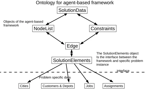
Ontology for agent-based framework SolutionData
Edge
Constraints
SolutionElements
Cities Jobs Assignments
The SolutionElements object Is the interface between the framework and specific problem instance
Problem specific data
interface Objects of the agent-based
framework
Problem specific objects inheriting from the abstract SolutionElements object
NodeList
[image:8.612.153.461.139.330.2]Customers & Depots
Figure 1: The combinatorial optimisation ontology
The ontology used by the framework generalises these notions as abstract
1
objects.
2
• SolutionElements: A SolutionElement is an abstract object that can
3
represent a problem specific object such as ajobin PFSP or, acustomer
4
or depot in CVRP.
5
• Edge: An Edge object contains two SolutionElements objects. These
6
are used to represent pairs of jobs orcustomers in a permutation that
7
will be in the cooperation protocol to identify good patterns in
improv-8
ing permutations.
9
• Constraints: The Constraints interface is between the high level
10
framework and the concrete constraints used by a specific problem.
11
These are used to verify a valid permutation.
12
• NodeList: A NodeList object is a list of SolutionElements objects or
13
Edges. It represents a schedule of jobs in the PFSP. In the case of
14
CVRP, a NodeList represents a Route and is therefore a sub-list of a
15
full permutation.
• SolutionData: A SolutionData object is a list of NodeList objects
1
and therefore is the permutation that is optimised by the framework.
2
In this study it represents aschedule of jobsin PFSP, or a collection of
3
routes in CVRP.
4
All message passing in the framework, including the whole ontology, is
5
written in XML. This can be advantageous as many benchmark problems,
6
these days, are also in XML making the interface between problem definition
7
and ontology seamless in practice. Figure 1 shows the structure of the
ontol-8
ogy and how SolutionElements are the interface between the framework and
9
a concrete problem.
10
3.3. Edge selection and short-term memory
11
The framework features a method of Edge selection and short-term
mem-12
ory. A conversation, as has been explained already, is a type of distributed
13
heuristic. Its purpose is to identify constituent features of incumbent
solu-14
tions that are likely to lead to the building of improving solutions.
15
This is achieved by using objects defined in the ontology. SolutionData
16
object in the ontology is built from the sub-objects of NodeLists and Edges
17
and SolutionElements. Thus to represent a permutation of n jobs for PFSP
18
a SolutionData object is built from one NodeList object and which itself is
19
made upn−1 Edges objects which are themselves built fromn
SolutionEle-20
ments. Similarly a CVRP representation ofncustomers is one Solution Data
21
object withx (this number is determined during the search) NodeLists. The
22
NodeLists are built of n−1 Edges and n SolutionElements.
23
If we take a permutation of the unique ID numbers of each the Solu-tionElements objects we can represent a SolutionData object with 10 ele-ments as follows: (3,4,6,7,5,8,9,0,1,2). Furthermore we can break this permutation into a collection of Edge objects:
(3,4),(4,6),(6,7),(7,5),(5,8),(8,9),(9,0),(0,1),(1,2),(2,3)
During a conversation each agent runs its metaheuristic and produces a
24
new incumbent solution. Each agent then breaks this solution into Edge
25
objects and sends then to one of the metaheuristic agents that has been
26
designated as the “initiator” for the duration of that conversation only. All
27
metaheuristic agents are exactly the same and have the potential to take on
28
the role of an initiator in a conversation.
The initiator agent collects all the Edge objects from all the other agents
1
into a list and scores them by frequency. Here, frequency is the number of
2
times an Edge appears in the initiators list. The only Edge objects that are
3
retained are the ones that have the same score as the number of agents that
4
are participating in the conversation. The idea here is that if an Edge occurs
5
frequently in all incumbent solutions, it is likely to be an Edge that will be
6
part of an improving solution. These retained good Edges are then shared
7
by the initiator with the other agents.
8
Another feature is the learning mechanism where each agent keeps a
short-9
term memory of good Edges. This is a queue of good Edges that operates
10
somewhat like a Tabu list. An agent’s queue is populated during the first
11
conversation with edges from the incumbent solution produced by its
meta-12
heuristic. Thereafter the queue is maintained at a factor, that is 20%, of
13
the size of the candidate solution for the problem instance at hand. In
sub-14
sequent conversations as new edges not already in the list arrive, they are
15
pushed onto the front of the queue while other edges are popped off the back
16
of the queue so that the size of the list does not change.
17
The Edges in the short-term memory are used at the start of each
con-18
versation to modify the performance of agent’s metaheuristic to enable it to
19
find better solutions.
20
The basic idea of this learning mechanism is that both the RandNEH and
21
RandCWS heuristics of (Juan et al., 2015) used in this study make use of
22
ordered lists to construct new solutions. These heuristics use biased random
23
functions to choose items from these lists. We use the Edges identified by
24
the learning mechanism to reorder these lists and so influence the way new
25
solutions are constructed.
26
4. IMPLEMENTATION 27
The framework is implemented using JADE (Bellifemine et al., 2007). It
28
allows a developer to concentrate on the function and behaviour of agents
29
while it handles inter-agent and inter-platform communication and
hus-30
bandry.
31
The configuration file of a launcher agent lists which problems are to be
32
solved. It also contains how many conversations the metaheuristic agents are
33
going to conduct for a particular problem.
34
At start-up, parameters determine which metaheuristic will be employed
35
as well as any parameter settings associated with it. Once the metaheuristic
agents have completed the set number of conversations they each send their
1
best result to the launcher agent. The launcher then prints an output file
2
with the best solution and objective function value.
3
The framework conducts a search where each agent is launched and
reg-4
isters with the JADE platform that hosts the framework. Once this is
com-5
plete, the agents wait for the launcher agent to read in a problem from file.
6
The launcher will then send the problem to each of the metaheuristic agents.
7
Only when the metaheuristic agents receive that problem from the launcher
8
do they embark on a search.
9
4.1. Heuristics used by the agents
10
In this study depending on whether they are solving PFSP or VRP, the
11
agents instantiate the heuristics developed by Juan et al. (2010b,a)
respec-12
tively.
13
In the case of PFSP, the metaheuristic used is the Randomised NEH
14
(RandNEH) algorithm of Juan et al. (2010b). It is a stochastic version of the
15
classic heuristic of Nawaz et al. (1983). Just as the NEH algorithm creates an
16
ordered list ofjobssorted from tardiest to quickest, the RandNEH algorithm,
17
instead of choosing jobs in order from the list, chooses them according to a
18
randomised process based on the Triangular probability distribution.
19
While for the CVRP, the metaheuristic used is the Randomised Clarke
20
Wright Savings (RandCWS) algorithm of Juan et al. (2010a). It is a
stochas-21
tic version of the classic savings heuristic of Clarke and Wright (1964). Rather
22
than generating new routes by choosing the greatest relevant saving from the
23
savings list, it chooses according to a Geometric distribution where the jth
24
savings from the list is chosen by a probabilistic function described in Juan
25
et al. (2010a).
26
Both these algorithms have been integrated into our system according to
27
our framework. This was quite a simple process where the heuristics
imple-28
ment the abstract objects defined in the scheduling and routing ontology.
29
For example, the Edge and Job objects of the RandNEH algorithm are now
30
subclasses of the Edge and SolutionElements abstract classes of the
frame-31
work. Similarly for VRP problems, where the Route, Edge and Customer
32
objects are now subclasses of the NodeElements, Edge and SolutionElements
33
objects of the framework.
34
This means we can use thegood Edgesfound as a result of aconversation
35
of the framework to modify the Job lists and Saving lists of the RandNEH
36
and RandCWS algorithms respectively.
In the case of PFSP, the list of Edges found by the agents is turned
1
into a list of SolutionElements (Jobs) where their order in the Edge list
2
is preserved. The Jobs list generated by the RandNEH algorithm is then
3
reordered with respect to the list of Jobs generated from the Edge list, with
4
the new Jobs being moved to the front of the list. This affects the operation
5
of the RandNEH algorithm where the new Jobs are likely be favoured in the
6
construction of any new improving schedule.
7
It is a similar process for the RandCWS algorithm. However this time
8
the Edges in Edge list are also Super Classes of the Edges in the savings
9
Savings List. Again the Savings List is reordered with respect to the Edge
10
list where these Edges are moved to the head of the Savings List. This again
11
affects the operation of the RandCWS algorithm favouring the good Edges
12
found as a result of the Agents’ conversations.
13
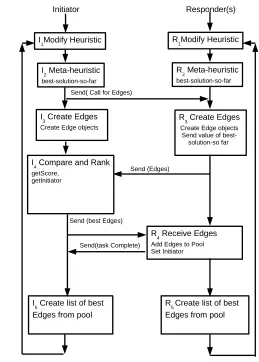
4.2. Description of a conversation
14
Figure 2 shows the edge selection protocol used by the metaheuristic
15
agents. One complete execution of the algorithm illustrated is aconversation.
16
In any conversation, there will be an agent that takes on the role of an
17
initiator and the others are responders. In the very first conversation agent1
18
will always take on the role of initiator. Thereafter, any agent can be the
19
initiator, but it is determined in the previous conversation which agent will
20
be the initiator for the current conversation (see below).
21
In Figure 2 an agent taking on the role of initiator starts a conversation.
22
At the start of a conversation, each agent either takes a list of Edge objects
23
generated from a previous conversation or from one generated by the launch
24
agent (see I1 and R1 in Figure 2).
25
The agents then find a new incumbent solutions using their given
heuris-26
tics in conjunction with the edges provided in the previous step (see I2 and
27
R2 in Figure 2).
28
The initiator breaks its incumbent solution into edges and then invites
29
the responder agents to do the same and send them to the initiator, I3 and
30
R3 of Figure 2.
31
The receiving agents also send the value of their best-so-far solution. This
32
will be used by the initiator to determine which agent will be the new initiator
33
in the next conversation (see I4 in Figure 2).
34
In I4, the initiator receives the Edge objects from the responding agents
35
and collects them together. Each Edge object is scored and ranked based on
36
frequency. This can be seen in box I4 of Figure 2 as the function getScore.
Initiator Responder(s)
I2 Meta-heuristic
best-solution-so-far
R2 Meta-heuristic
best-solution-so-far
R3 Create Edges
Create Edge objects Send value of best-solution-so far
I4 Compare and Rank
getScore, getInitiator
R4 Receive Edges
Add Edges to Pool Set Initiator
I5 Create list of best Edges from pool
R5 Create list of best Edges from pool
Send( Call for Edges)
Send (Edges)
Send (best Edges)
Send(task Complete)
I3 Create Edges
Create Edge objects
[image:13.612.170.429.141.503.2]I1Modify Heuristic R1Modify Heuristic
Figure 2: The Cooperation Protocol showing one iteration of a conversation
In I4 of Figure 2, through the function getInitiator, the initiator also
de-1
termines which metaheuristic agent is going to be the initiator in the next
2
conversation. This is achieved by choosing the agent the best objective
func-3
tion value to be the initiator.
4
The initiator then sends good Edge objects, found during this
conversa-5
tion, to the receiving metaheuristic agents.
6
Each agent keeps a pool or short-term memory of high scoring Edge
7
objects. The pool acts as a sort of queue and its length is set when the agent
is launched. In this study all the agents have a pool size of 20% of length
1
of the instance currently being optimised. During the first conversation each
2
agent populates its pool as good edges are identified. Once the pool is up to
3
size, it is maintained as a queue as described in Section 3.3.
4
The other metaheuristic agents receive the lists of Edge objects from the
5
initiator (see box R4 in Figure 2). They also update their internal memory’s
6
or pools as described above. In box I5 and R5 of Figure 2, both initiator
7
and responder metaheuristic agents then each create a new solution by using
8
edges from their updated internal pools. These good edges are passed to the
9
metaheuristic the agent is configured to execute in the current search. The
10
metaheuristic uses these good edges when it is next called at the start of the
11
next conversation (back to I1 and R1 of Figure 2). This process repeats and
12
continues until the number of conversations set from the launcher agent are
13
completed.
14
5. EXPERIMENTAL DESIGN 15
In this section we discuss the experimental design.
16
5.1. Launcher agent
17
One launcher agent is invoked in each run. The launcher agent reads
18
from a configuration file the number of agents to be instantiated (see Section
19
5.4) as well as the number of conversations that will be conducted during the
20
test.
21
The launcher agent executes a construction heuristic to build an initial
22
solution for each instance and run: for PFSP a biased-randomised version
23
of the NEH algorithm (Nawaz et al., 1983) with Taillard’s speedups
imple-24
mented by (Juan et al., 2010b); and for CVRP, the Randomised CW Savings
25
algorithm (Juan et al., 2014, 2010a). This initial solution is passed on to
26
each of the individual agents.
27
5.2. The number of conversations
28
Juan et al. (Juan et al., 2010b, 2014, 2010a) suggested that, to be
effec-29
tive, the RandNEH and RandCWS heuristics should be run for a maximum
30
time of about 2.5 minutes. We benchmarked their code and observed the
31
same phenomena, hence used the same running time on our machine during
32
our experiments.
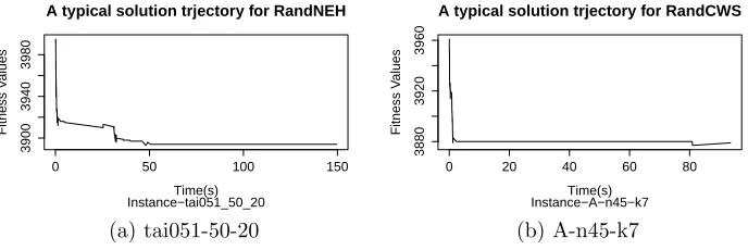
0 50 100 150
3900
3940
3980
A typical solution trjectory for RandNEH
Instance−tai051_50_20Time(s)
Fitness V
alues
(a) tai051-50-20
0 20 40 60 80
3880
3920
3960
A typical solution trjectory for RandCWS
Instance−A−n45−k7Time(s)
Fitness V
alues
[image:15.612.130.474.142.257.2](b) A-n45-k7
Figure 3: Typical Solution trajectories of the RandNEH and RandCWS algorithms
This gave us a guide as to how long our system should be run and
there-1
fore determine the number of conversations that would be needed. The time
2
taken for the agents to complete a conversation is mainly governed by the
3
time taken for an agent’s given heuristic to execute. To this end, we
con-4
ducted tests showing that both heuristics typically have a period of maximum
5
improvement of about 12 seconds. As an example, Figure 3 plots the solution
6
trajectories of the PFSP instance tai051 and the CVRP instance A-n45-k9
7
against time. We can see that these algorithms have their period of greatest
8
improvement in about the first 12 seconds of operation. Thus we determined
9
that the system should execute 10 conversations for our system to run for
10
about the same time as the standalone versions of the RandNEH and
Rand-11
CWS heuristics. This would also take into account any lag caused by the
12
asynchronous nature of the system.
13
5.3. Parameter Settings
14
Since the RandCWS and RandNEH methods of Juan et al. were already
15
written in JAVA, they were integrated with minimum effort as a module
16
of our agent based system. They utilise the edge selection heuristic of the
17
agent-based system by taking edges identified during each conversation and
18
re-ordering the jobs list of the RandNEH algorithms and the savings list of
19
the RandCWS algorithm as explained in Section 4.1.
20
Both algorithms use a random seed which is a number which introduces
21
a bias to a random number generator. In the tests for both the PFSP and
22
CVRP, each agent is configured with exactly the same random seeds (Juan
23
et al., 2010a,b).
However in their article Juan et al. (2011) describe how they combined
1
Monte-Carlo simulation techniques with the Clarke Wright Savings algorithm
2
to develop the probabilistic RandCWS algorithm. It was designed so that it
3
would require little parameter tuning. To this end they describe a parameter
4
α that is used to define different geometric distributions. Such a distribution
5
can then used by the RandCWS heuristic to choose the next edge from the
6
Clarke Wright Savings list as part of its solution building process. The α
7
-parameter is itself chosen at random from a uniform distribution between
8
two values (a, b) where 0 < a ≤ b < 1. In their paper, Juan et al choose
9
α-values from the intervalα∈ {0.05−0.25}. They show that for anyα-value
10
in this interval, the algorithm will give similar and good performance. In
11
correspondence with the authors, it was confirmed that the algorithm will
12
perform less well forα-values of above 2.3, while at the other end of the range
13
α-values close to the 0.05 will perform as any in the cited interval.
14
The intuitive idea for spreading theα−values is to maximise the use of
15
different distributions during a search. While these choices do not effect the
16
solution quality it means the agents will produce slightly different solutions
17
which will produce different edges that will enhance the performance of the
18
distributed edge selection algorithm.
19
In both case studies each metaheuristic is allowed to run for 12 seconds
20
each time it is called.
21
Following Juan et al. (2014, 2013) in what we call our standalone
ex-22
periments, that is the traditional case without cooperative search being
23
used, we compare our cooperating agents with the stand alone by
run-24
ning the experiments for each group for a maximum time of 40 minutes
25
to match the computational effort of the system running 16 agents i.e.
26
16×150s = 2400s (40mins). Thus all agents versus standalone comparisons
27
are made against this worst case scenario.
28
5.4. Experimental set-up
29
The main hypothesis to be tested in these experiments is that cooperating
30
agents produce better results than their stand alone equivalents. The results
31
are also compared with state-of-art results for each of these benchmarks. To
32
this end, for each instance of the tests the following scenarios were run:
33
The CVRP tests were conducted as follows with α−values selected on
34
0.01 increments from the set {0.03 to 0.18} 35
• Stand alone agent: 1 metaheuristic agent where the α−value= 0.03
• 4 agents: α∈ {0.03−0.06} 1
• 8 agents: α∈ {0.03−0.1} 2
• 12 agents: α∈ {0.03−0.14} 3
• 16 agents:α∈ {0.03−0.18} 4
The PFSP tests were conducted similarly but without the need for α− 5
values.
6
They are tested in this way so that standalone agents running just one
7
metaheuristic at a time can be compared statistically with groups of
coop-8
erating agents in order to test the main hypothesis.
9
Every instance is tested 20 times. The resulting values are then used to
10
evaluate the performance of the test. In particular the average and minimum
11
value of the 20 runs for each problem are taken. These are compared with
12
the known optimal or best values for each problem instance.
13
To test the hypothesis that agents cooperating by edge selection perform
14
better than stand alone agents, Wilcoxon signed rank tests are conducted
15
for each benchmark instance, with a 95% confidence level. We used the
16
Wilcoxon test rather than t-test because we cannot guarantee that the test
17
results will be normally distributed Moore and McCabe (1989). These tests
18
compare the difference between the distributions of 16, 12, 8, and 4 agents
19
cooperating with the stand alone agents. A secondary hypothesis is explored
20
where the performances of groups of 4, 8, 12 and 16 agents are compared using
21
the Wilcoxon signed rank test to ascertain whether increasing the number
22
of agents results in better performance. The following notation is used in
23
tables 2, 3, 6 and 7. Given two algorithms (or different settings for the same
24
algorithm); A versus B, > (<) denotes that A (B) is better than B (A) and
25
this performance difference is statistically significant at a 95% confidence
26
level. However, ≥ (≤) denotes that A (B) is better than B (A) although
27
statistical significance could not be supported. Lastly, ≈ denotes the case
28
where both approaches consistently achieve the same value.
29
The results for each problem are averaged and the average percentage
30
deviation from the known optimum is calculated. The percentage deviation
31
from a known optimum is calculated in the standard manner:
32
M ethodsolution−Bestsolution
Bestsolution
The results are also analysed to find the best result of each group of agents
1
over the 20 runs of each problem instance.
2
Juan et al. (2014, 2013)
3
5.5. Machines
4
All tests are run on the same Linux cluster using 8 identical machines;
5
two agents were run per-node of the cluster. The agents are configured to
6
use 2 GB of memory.
7
6. RESULTS OF EXPERIMENTS 8
6.1. Permutation Flow-shop Scheduling results
9
Table 1 shows the average percentage deviation from the best known or
10
optimum value for each of the benchmark instances tested, as well as the
11
percentage deviation for the best value found across the 20 runs. The table
12
also compares our results with the Hybrid Genetic algorithm of Zobolas et al.
13
(2009). Here the average value reported by Zobolas et al. (2009) is given as a
14
percentage deviation from the best known solution (BKS). Despite the fact
15
that this is a type of hyper-heuristic system where the only parameter tuning
16
is the number of conversations executed, the PFSP results are competitive
17
with the state-of-the-art results for these problem instances. It is only in the
18
larger three instances where our average deviation is not better than that of
19
Zobolas et al. (2009).
[image:18.612.113.493.497.620.2]20
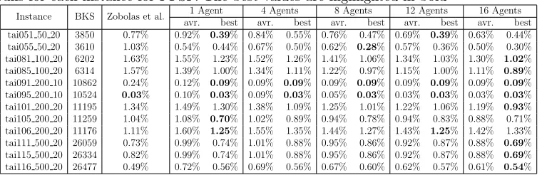
Table 1: The average (avr.) and best percentage deviation from the upper bound over 20 runs for each instance for PFSP. The best values are highlighted in bold
Instance BKS Zobolas et al. 1 Agent 4 Agents 8 Agents 12 Agents 16 Agents avr. best avr. best avr. best avr. best avr. best tai051 50 20 3850 0.77% 0.92% 0.39% 0.84% 0.55% 0.76% 0.47% 0.69% 0.39% 0.63% 0.44% tai055 50 20 3610 1.03% 0.54% 0.44% 0.67% 0.50% 0.62% 0.28% 0.57% 0.36% 0.50% 0.30% tai081 100 20 6202 1.63% 1.55% 1.23% 1.52% 1.26% 1.41% 1.06% 1.34% 1.03% 1.30% 1.02% tai085 100 20 6314 1.57% 1.39% 1.00% 1.34% 1.11% 1.22% 0.97% 1.15% 1.00% 1.11% 0.89% tai091 200 10 10862 0.24% 0.12% 0.09% 0.09% 0.09% 0.09% 0.09% 0.09% 0.09% 0.09% 0.09% tai095 200 10 10524 0.03% 0.10% 0.03% 0.09% 0.03% 0.05% 0.03% 0.03% 0.03% 0.03% 0.03% tai101 200 20 11195 1.34% 1.49% 1.30% 1.38% 1.09% 1.25% 1.01% 1.22% 1.06% 1.19% 0.93% tai105 200 20 11259 1.04% 1.08% 0.70% 1.02% 0.89% 0.94% 0.78% 0.94% 0.83% 0.88% 0.71% tai106 200 20 11176 1.11% 1.60% 1.25% 1.55% 1.35% 1.44% 1.27% 1.43% 1.25% 1.42% 1.33% tai111 500 20 26059 0.73% 0.99% 0.74% 1.01% 0.88% 0.95% 0.86% 0.92% 0.87% 0.88% 0.69% tai115 500 20 26334 0.82% 0.99% 0.74% 1.01% 0.88% 0.95% 0.86% 0.92% 0.87% 0.88% 0.69% tai116 500 20 26477 0.49% 0.72% 0.56% 0.69% 0.56% 0.67% 0.60% 0.62% 0.57% 0.61% 0.54%
With respect to answering our main hypothesis: “is cooperation by
pat-21
tern matching better than no cooperation?”, we compared 4 agents
cooper-22
ating against a stand alone agent (see Section 5.3). In addition we wanted
to test if increasing the number of agents produced a statistically significant
1
improvement in the results. Tables 2 and 3 list these results; in each case we
2
tested for statistical significance.
3
In table 2, with the exception of thetai055 50 20 instance, it can be seen
4
that groups of 8,12 and 16 agents perform better than the stand alone with
5
statistical significance. However, for the tai055 50 20 instance, 16 agents
6
show some improvement, if not statistically, over the stand alone.
Further-7
more, two instances of 4 agents perform statistically better than the
stan-8
dalone but the rest all show some improvement but not at the 95% level.
[image:19.612.111.375.297.490.2]9
Table 2: Table showing cooperating agents performing better than the standalone equiv-alent at the 95% in PFSP
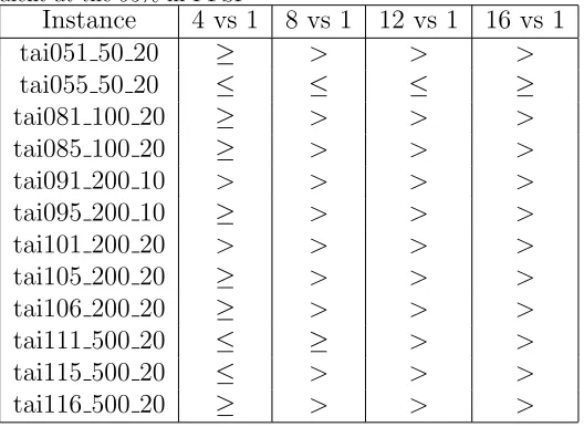
Instance 4 vs 1 8 vs 1 12 vs 1 16 vs 1
tai051 50 20 ≥ > > >
tai055 50 20 ≤ ≤ ≤ ≥
tai081 100 20 ≥ > > >
tai085 100 20 ≥ > > >
tai091 200 10 > > > >
tai095 200 10 ≥ > > >
tai101 200 20 > > > >
tai105 200 20 ≥ > > >
tai106 200 20 ≥ > > >
tai111 500 20 ≤ ≥ > >
tai115 500 20 ≤ > > >
tai116 500 20 ≥ > > >
Table 3 explores the possibility that adding more agents leads to better
10
results. Here we can see that 8 agents perform statistically better than 4,
11
while 12 agents show some improvement, but not statistically, over 8. The
12
same is true for 16 over 12 agents. However the instances tai091 200 10 and
13
tai105 200 20 achieve statistical significance as well. By the time we get to
14
16 versus 4 agents, 16 agents always perform statistically better except for
15
tai091 200 10 where statistical significance is not reached. It should also be
16
noted for tai091 200 10 while the cooperating agents perform better than
17
the stand alone, thereafter the all achieve the same value. It is clear that
18
progressively increasing the number of agents from 4 to 8 to 12 to 16 results
19
in an increase in performance. However this improvement is not always
20
statistically significant. If we consider the column of the table where 16
agents are compared with 8 we see that the level of improvement gains more
1
significance. This is suggestive that it is better to increase the number of
2
agents by a factor of 2.
[image:20.612.113.432.212.402.2]3
Table 3: Table showing different groups cooperating agents perform at the 95% confidence level in PFSP
Instance 8 vs 4 12 vs 8 16 vs 12 16 to 8 16 to 4
tai051 50 20 > ≥ ≥ > >
tai055 50 20 > ≥ > > >
tai081 100 20 > ≥ ≥ > >
tai085 100 20 > ≥ ≥ > >
tai091 200 10 ≈ ≈ ≈ ≈ ≥
tai095 200 10 > ≥ ≥ ≈ >
tai101 200 20 > ≥ ≥ ≥ >
tai105 200 20 > ≤ > > >
tai106 200 20 > ≥ ≥ ≥ >
tai111 500 20 > > ≥ > >
tai115 500 20 > ≥ ≥ ≥ >
tai116 500 20 > > ≥ > >
The cooperation mechanism used in this study works by identifying and
4
sharing of good patterns that form partial solutions to the problem at hand.
5
These are then passed to a metaheuristic to build a new putative solution
6
to the problem. Given this, it is interesting to study the patterns (edges)
7
identified by each agent and compare them to the final solution found by the
8
system. To this end, the final permutation (Edges which appear in the final
9
solution and are identified during the search (see table 4)are highlighted in
10
bold) <12, 37, 20, 31, 39,35, 34, 6, 40, 5, 10, 1, 7, 15, 33, 43, 24, 42, 27,
11
29, 46, 47, 36, 23, 14, 2, 44, 8, 45, 17, 13, 22, 21, 48, 18, 28, 16, 49, 38, 19,
12
26, 41, 11, 32, 25, 9, 30, 4, 50,3> of jobs found by the system during one
13
run of the tai051 50 20 instance is compared with the patterns in table 4.
14
These are all the unique edges identified during this search. These edges are
15
identified multiple times but the table only shows them once.
16
Indeed some edges (highlighted in bold) identified by the system do end
17
up in the final job permutation. Furthermore, we can identify linked edges
18
such as 50, 3, 12 at the end and beginning of the permutation. However
19
these are not as many as seen with CVRP results below because of the way
20
the makespan 4 is calculated as a special cumulative sum of columns of jobs.
Table 4: Patterns found by 4 cooperating agents PFSP for problem tai051 50 20.
Agents Edges
agent1 (14,15) (4,25) (32,22) (39,16) (25,50) (19,41) (13,32) (44,45) (45,6) (50,3) (28,38) agent2 (35,34) (9,30) (5,10) (2,44) (12,37) (1,7) (4,50) (10,1) (24,42) (50,3) agent3 (3,12) (37,39) (30,46) (50,3) (35,15) (41,7) (34,33) (38,24) (47,23) (42,49) agent4 (40,21)(22,13)(6,42) (33,40) (26,2) (5,14) (7,18) (37,28)(39,35)(44,11)
6.2. Capacitated Vehicle Routing results
1
Table 5 compares the percentage deviation for average and best results for
2
the different groups of agents from the best known solution. The table also
3
compares our percentage deviations for these problem instances with those of
4
Altınel and ¨Oncan (2005) (donated by A) and Juan et al. (2010b) (denoted
5
by B). However, Juan et al. (2010b) only has results for a selection of the
6
instances we tested. They represent the latest work on these benchmark
7
instances so we have included them for comparison. Comparing our results
8
with those of Altınel and ¨Oncan (2005) and Juan et al. (2010b) we can
9
see that agents improve on their results. Furthermore, to the best of our
10
knowledge, in four cases we have found results that are better than the
11
current best known solutions. A−n39−k6,A−n45−k7,A−n55−k9 and
12
A−n63−k9 are highlighted in italics for the best average value and in best
13
for our best overall score.
14
Table 5: The average (avr.) and best percentage deviation from the optimum/upper bound over 20 runs for each instance for CVRP
Instance BKS A and B Juan et al. avr.1 Agentbest avr.4 Agentsbest avr.8 Agentsbest 12 Agentsavr. best avr.16 Agentsbest
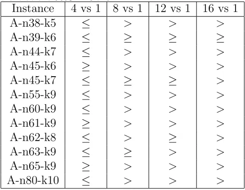
A-n38-k5 734.18 3.577% 0.54% 0.07% 0.04% 0.09% 0.04% 0.02% -0.03% -0.02% -0.03% -0.03% -0.03% A-n39-k6 833.14 2.233% - 0.01% 0.01% 0.01% 0.01% 0.01% 0.01% 0.01% 0.01% 0.01% 0.01% A-n44-k6 939.33 2.394% - 0.63% 0.57% 0.70% 0.57% 0.55% 0.39% 0.40% 0.29% 0.32% -0.12% A-n45-k6 944.88 1.383% - 0.92% 0.92% 0.92% 0.92% 0.69% 0.00% 0.20% 0.00% 0.00% 0.00% A-n45-k7 1147.28 1.842% 0.07% 0.05% -0.03% 0.07% -0.02% 0.03% -0.03% 0.03% -0.03% -0.01% -0.48% A-n55-k9 1074.46 2.378% 0.14% 0.13% 0.05% 0.26% 0.05% 0.06% 0.05% 0.05% 0.05% 0.05% 0.05% A-n60-k9 1355.80 1.64% 0.13% 0.50% 0.50% 0.50% 0.50% 0.46% 0.22% 0.40% 0.22% 0.37% 0.22% A-n61-k9 1039.08 1.654% 0.49% 0.27% 0.26% 0.26% 0.26% 0.25% 0.13% 0.23% 0.12% 0.22% 0.12% A-n62-k8 1294.28 4.648% - 0.70% 0.62% 0.76% 0.62% 0.62% 0.62% 0.65% 0.62% 0.62% 0.62% A-n63-k9 1619.90 2.051% - 0.75% 0.45% 0.88% 0.69% 0.73% 0.40% 0.53% 0.14% 0.32% 0.14% A-n65-k9 1181.69 2.392% 0.66% 1.06% 1.05% 1.05% 0.72% 0.92% 0.28% 0.82% 0.64% 0.61% 0.14% A-n80-k10 1766.50 2.952% 0.2% 1.04% 0.99% 1.04% 0.99% 0.98% 0.77% 0.87% 0.77% 0.85% 0.70%
Again we tested for the main hypothesis. We compared groups of 4, 8,
15
12,and 16 agents cooperating against a stand alone agent. As before we
16
tested for statistical significance using the Wilcoxon signed rank test at the
17
95% confidence level. Table 6 lists these result using the same notation as
18
used in table 2 above. As with the PFSP, 4 agents cooperating do not show
any improvement from their stand alone equivalent. However, groups of 8, 12
1
and 16 agents with increasing certainty perform better than the stand alone
2
agent. Indeed 16 agents all perform better a 95% confidence level except for
3
the A−n39−k6 instance.
[image:22.612.110.357.224.416.2]4
Table 6: Table showing cooperating agents performing better than the standalone equiv-alent at the 95% in CVRP
Instance 4 vs 1 8 vs 1 12 vs 1 16 vs 1
A-n38-k5 ≤ > > >
A-n39-k6 ≤ ≥ ≥ ≥
A-n44-k7 ≤ > > >
A-n45-k6 ≥ > > >
A-n45-k7 ≤ ≥ ≥ >
A-n55-k9 ≤ > > >
A-n60-k9 ≤ > > >
A-n61-k9 ≥ > > >
A-n62-k8 ≤ > ≥ >
A-n63-k9 ≤ ≥ > >
A-n65-k9 ≥ > > >
A-n80-k10 ≤ > > >
In table 7 we report the results of our tests for the secondary hypothesis.
5
As with the PFSP results, we can see a gradual improvement as more agents
6
are added. But again it seems it is necessary to double the number of agents
7
each time in order to observe improvement in results. The addition of 4
8
agents each time results in an improvement that is not always statistically
9
significant. However if the agents are doubled each time in groups of 4, 8
10
and 16 there is a greater proportion of statistically significant improvement
11
from the additive case.
12
Finally, we show the patterns generated for a sample on problem instance
13
A−n38−k5 in table 9 and compare them to the final result of this run in
14
table 8. We highlight in bold those edges identified by the agents in table
15
9 that end up in the final solution in table 8. As can be seen there are
16
many more such edges than for the PFSP. This is because the relationship
17
between edges and cities is much more direct in the case of CVRP as costs
18
are calculated as 2D-euclidean distances between cities.
19
From this study we conclude that with no parameter tuning between
20
case studies our system can produce results which are commensurate with
Table 7: Table showing different groups cooperating agents perform at the 95% confidence level in CVRP
Instance 8 vs 4 12 vs 8 16 vs 12 16 vs 8 16 vs 4
A-n38-k5 > > > > >
A-n39-k6 ≥ ≥ ≥ ≥ ≥
A-n44-k7 > > > > >
A-n45-k6 > > > > >
A-n45-k7 > ≥ ≥ ≥ >
A-n55-k9 > ≥ ≥ ≥ >
A-n60-k9 > ≥ ≥ > >
A-n61-k9 > ≥ ≥ ≥ >
A-n62-k8 > ≤ ≥ ≥ >
A-n63-k9 > > > > >
A-n65-k9 > ≥ > > >
[image:23.612.111.373.429.519.2]A-n80-k10 > > ≥ > >
Table 8: Final Solution to CVRP problem A-n38-k5.
Route Name Routes
Route1 [1, 8, 6, 12, 28, 23, 33, 1] Route2 [1, 27, 13, 4, 2, 5, 17, 26, 7, 30, 1] Route3 [1, 9, 34, 36, 24, 31, 11, 22, 1] Route4 [1, 10, 18, 37, 14, 16, 3, 15, 25, 1] Route5 [1, 21, 38, 32, 29, 35, 20, 19, 1]
Table 9: Patterns found by 4 cooperating agents for CVRP problem A-n38-k5.
Agents Edges
agent1 (35,20)(38,32) (29,35) (20,19) (21,38) (32,29) (1,21) (19,1) agent2 (30,31) (11,1) (1,19)(31,11) (35,30) (19,35)
the state-of-the-art studies in both fields. Furthermore, in four instances with
1
the CVRP tests we were able to the best of our knowledge beat the current
2
best results for these instances. We were also able to show for groups of 8, 12
3
and 16 agents compared with the stand alone equivalent, that cooperation
4
by pattern finding is better than no cooperation. Finally we are also able to
5
show that doubling the number agents each time leads to improving results
6
as shown in Figure 4.
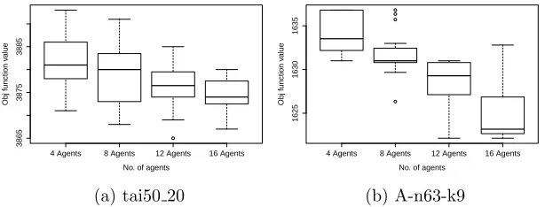
7
4 Agents 8 Agents 12 Agents 16 Agents
3865
3875
3885
No. of agents
Obj function v
alue
(a) tai50 20
4 Agents 8 Agents 12 Agents 16 Agents
1625
1630
1635
No. of agents
Obj function v
alue
[image:24.612.149.456.264.381.2](b) A-n63-k9
Figure 4: Boxplots of objective values obtained in 10 runs for 16, 12, 8 and 4 agents on a selected instance from the (a) STSP, (b) PFSP, and (c) CVRP problem domains.
7. CONCLUSION 8
In this study we propose a general agent-based distributed framework
9
where each agent implements a different metaheuristic/local search
combi-10
nation. An agent continuously adapts itself during the search process using
11
a cooperation protocol based on reinforcement learning and pattern finding.
12
Good patterns that make up improving solutions are identified by frequency
13
of occurrence in a conversation and shared with the other agents. The
frame-14
work has been tested on well known benchmark problems for two tests cases
15
PFSP and CVRP. In both cases, with no parameter tuning between domains,
16
the platform performed at least as well as the state-of-art. For CVRP, we
17
were able, in cases of A−n38−k5,A−n44−k6 andA−n45−k7 to improve
18
on the best known solutions for these instances1.
19
We have also shown eight or more agents perform better than a stand
1
alone agent with a 95% confidence level. Furthermore, we have shown with a
2
reasonable level or certainty, if not always with 95% confidence, that an
im-3
provement in performance can be achieved each time you double the number,
4
up to 16, agents used.
5
The distributed computing framework presented can be run on a local
6
network of personal computers each using 2GB memory.
7
The framework also aims to be a generic and modular needing very little
8
parameter tuning across different problem types tested so far. It has been
9
been applied successfully to PFSP and CVRP. It has also been used to model
10
fairness in Nurse Rostering (Martin et al., 2013) using real-world data. This
11
flexibility is achieved by means of an ontology which enables the agents to
12
represent these problems with the same internal structure.
13
This is an interesting and little researched topic that warrants further
14
investigation such as: extending the ontology to apply the framework to
15
new problems; adding more heuristics and metaheuristics and improving the
16
pattern finding protocol.
17
Finally, this framework will be published as an open source project so that
18
other metaheuristics and cooperation protocols can be added and tested by
19
other researchers. The project is called MACS (Multi-agent Cooperative
20
Search) and will be published at the following website: http://www.cs.
21
stir.ac.uk/~spm/.
22
8. Acknowledgement 23
The study was funded EPSRC Dynamic Adaptive Automated Software
24
Engineering (DAASE) project EP/J017515/1.
25
9. Appendix A. Supplementary material 26
Supplementary data associated with this article can be found, in the
27
online version, at: www.tobeprovided.ac.uk
28
10. References 29
˙I. K. Altınel and T. ¨Oncan. A new enhancement of the clarke and wright
30
savings heuristic for the capacitated vehicle routing problem. Journal of
31
the Operational Research Society, 56(8):954–961, 2005.
P. Augerat, J.M. Belenguer, E Benavent, A. Corber´an, D. Naddef, and G.
Ri-1
naldi. Computational results with a branch and cut code for the
capaci-2
tated vehicle routing problem. Rapport de recherche- IMAG, 1995.
3
M. Aydin and T.C. Fogarty. A distributed evolutionary simulated annealing
4
algorithm for combinatorial optimisation problems. Journal of Heuristics,
5
10(3):269–292, 2004a.
6
M. Aydin and T.C. Fogarty. Teams of autonomous agents for job-shop
7
scheduling problems: An experimental study. Journal of Intelligent
Man-8
ufacturing, 15(4):455–462, 2004b.
9
D. Barbucha. A cooperative population learning algorithm for vehicle routing
10
problem with time windows. Neurocomputing, 146:210–229, 2014.
11
F. L. Bellifemine, G. Caire, and D. Greenwood. Developing multi-agent
sys-12
tems with JADE. Wiley, 2007. ISBN 0470057475.
13
C. Blum and A. Roli. Metaheuristics in combinatorial optimization:
14
Overview and conceptual comparison. ACM Computing Surveys (CSUR),
15
35(3):268–308, 2003.
16
E.K. Burke, M. Gendreau, M. Hyde, G. Kendall, G. Ochoa, E. ¨Ozcan, and
17
R. Qu. Hyper-heuristics: A survey of the state of the art. Journal of the
18
Operational Research Society, 64(12):1695–1724, 2013.
19
G. Clarke and J.W. Wright. Scheduling of vehicles from a central depot to a
20
number of delivery points. Operations research, 12(4):568–581, 1964.
21
S. H. Clearwater, T. Hogg, and B. A. Huberman. Cooperative problem
22
solving. Computation: The Micro and the Macro View, pages 33–70, 1992.
23
T. Crainic and M. Toulouse. Explicit and emergent cooperation schemes for
24
search algorithms. Learning and intelligent optimization, pages 95–109,
25
2008.
26
G.B. Dantzig and J.H. Ramser. The truck dispatching problem.Management
27
Science, 6:80–91, 1959.
28
N. El Hachemi, T. G. Crainic, N. Lahrichi, W. Rei, and T. Vidal. Solution
29
integration in combinatorial optimization with applications to cooperative
30
search and rich vehicle routing. 2014.
FIPA. Fipa iterated contract net interaction protocol specification, 2009.
1
URL http://www.fipa.org/specs/fipa00030/index.html.
2
M. R. Garey, D. S. Johnson, and R. Sethi. The complexity of flowshop
3
and jobshop scheduling. Mathematics of operations research, 1(2):117–129,
4
1976.
5
M.R. Garey and D.S. Johnson. Computers and Intractability, A Guide to the
6
Theory of NP-Completeness. Bell Telephone Laboratories Inc., 1979.
7
T. R. Gruber. A translation approach to portable ontology specifications.
8
Knowledge acquisition, 5(2):199–220, 1993.
9
T. Hogg and C. P. Williams. Solving the really hard problems with
co-10
operative search. In Proceedings of the National Conference on Artificial
11
Intelligence, pages 231–231, 1993.
12
F. Hutter, D. Babic, H.H. Hoos, and A. J. Hu. Boosting verification by
13
automatic tuning of decision procedures. InFormal Methods in Computer
14
Aided Design, 2007. FMCAD’07, pages 27–34. IEEE, 2007.
15
A. A. Juan, J. Faulin, R. Ruiz, B. Barrios, and S. Caball´e. The sr-gcws hybrid
16
algorithm for solving the capacitated vehicle routing problem. Applied Soft
17
Computing, 10(1):215–224, 2010a.
18
A A. Juan, J. Faul´ın, J. Jorba, D. Riera, D. Masip, and B. Barrios. On the use
19
of monte carlo simulation, cache and splitting techniques to improve the
20
clarke and wright savings heuristics. Journal of the Operational Research
21
Society, 62(6):1085–1097, 2011.
22
A. A. Juan, J. Faulin, J. Jorba, J. Caceres, and J. M. Marqu`es. Using parallel
23
& distributed computing for real-time solving of vehicle routing problems
24
with stochastic demands. Annals of Operations Research, 207(1):43–65,
25
2013.
26
A. A. Juan, Helena R. Louren¸co, M. Mateo, R. Luo, and Q. Castella. Using
27
iterated local search for solving the flow-shop problem: Parallelization,
28
parametrization, and randomization issues. International Transactions in
29
Operational Research, 21(1):103–126, 2014.
A.A. Juan, R. Ru´ız, H. R. Louren¸co, M. Mateo, and D. Ionescu. A
simulation-1
based approach for solving the flowshop problem. In Proceedings of the
2
Winter Simulation Conference, pages 3384–3395. Winter Simulation
Con-3
ference, 2010b.
4
A.A. Juan, J. Faulin, S. E Grasman, M. Rabe, and G. Figueira. A review of
5
simheuristics: Extending metaheuristics to deal with stochastic
combina-6
torial optimization problems. Operations Research Perspectives, 2:62–72,
7
2015.
8
A. Kouider and B. Bouzouia. Multi-agent job shop scheduling system based
9
on co-operative approach of idle time minimisation. International Journal
10
of Production Research, 50(2):409–424, 2012.
11
M. L´opez-Ib´anez, J. Dubois-Lacoste, T. St¨utzle, and M. Birattari. The irace
12
package, iterated race for automatic algorithm configuration. IRIDIA,
13
Universit´e Libre de Bruxelles, Belgium, Tech. Rep. TR/IRIDIA/2011-004,
14
2011.
15
R. Malek. An agent-based hyper-heuristic approach to combinatorial
op-16
timization problems. In Intelligent Computing and Intelligent Systems
17
(ICIS), 2010 IEEE International Conference on, volume 3, pages 428–434,
18
2010.
19
S.P. Martin, D. Ouelhadj, P. Smet, G Vanden Berghe, and E. ¨Ozcan.
Coop-20
erative search for fair nurse rosters. Expert Systems with Applications, 40
21
(16):6674–6683, 2013.
22
D. Meignan, J.C. Creput, and A. Koukam. A coalition-based
metaheuris-23
tic for the vehicle routing problem. In Evolutionary Computation, 2008.
24
CEC 2008.(IEEE World Congress on Computational Intelligence). IEEE
25
Congress on, pages 1176–1182. IEEE, 2008.
26
D. Meignan, A. Koukam, and J. C. Cr´eput. Coalition-based metaheuristic:
27
a self-adaptive metaheuristic using reinforcement learning and mimetism.
28
Journal of Heuristics, pages 1–21, 2010. ISSN 1381-1231.
29
M. Milano and A. Roli. Magma: A multiagent architecture for
metaheuris-30
tics. Systems, Man, and Cybernetics, Part B: Cybernetics, IEEE
Trans-31
actions on, 34(2):925–941, 2004. ISSN 1083-4419.
David S Moore and George P McCabe. Introduction to the Practice of
Statis-1
tics. WH Freeman/Times Books/Henry Holt & Co, 1989.
2
M. Nawaz, E. E. Enscore Jr, and I. Ham. A heuristic algorithm for the
m-3
machine, n-job flow-shop sequencing problem. Omega, 11(1):91–95, 1983.
4
D. Ouelhadj and S. Petrovic. A cooperative hyper-heuristic search
frame-5
work. Journal of Heuristics, 16(6):835–857, 2010.
6
M. Pinedo. Scheduling: theory, algorithms, and systems. Prentice-Hall, New
7
Jersey, 2002.
8
J. Ries and P. Beullens. A semi-automated design of instance-based fuzzy
pa-9
rameter tuning for metaheuristics based on decision tree induction.Journal
10
of the Operational Research Society, 66(5):782–793, 2015.
11
P Ross. Hyper-heuristics. InSearch Methodologies, pages 611–638. Springer,
12
2014.
13
E. Taillard. Benchmarks for basic scheduling problems. European Journal of
14
Operational Research, 64(2):278–285, 1993.
15
E. G. Talbi and V. Bachelet. Cosearch: A parallel cooperative metaheuristic.
16
Journal of Mathematical Modelling and Algorithms, 5(1):5–22, 2006. ISSN
17
1570-1166.
18
M. Toulouse, K. Thulasiraman, and F. Glover. Multi-level cooperative search:
19
A new paradigm for combinatorial optimization and an application to
20
graph partitioning. Euro-Par’99 Parallel Processing, pages 533–542, 1999.
21
E. Vallada and R. Ruiz. Cooperative metaheuristics for the permutation
22
flowshop scheduling problem. European Journal of Operational Research,
23
193(2):365–376, 2009.
24
X. F. Xie and J. Liu. Multiagent optimization system for solving the
trav-25
eling salesman problem (tsp). Systems, Man, and Cybernetics, Part B:
26
Cybernetics, IEEE Transactions on, 39(2):489–502, 2009.
27
G.I. Zobolas, C. D. Tarantilis, and G. Ioannou. Minimizing makespan in
28
permutation flow shop scheduling problems using a hybrid metaheuristic
29
algorithm. Computers & Operations Research, 36(4):1249–1267, 2009.