Experimental study of oscillating grid turbulence interacting with a solid boundary

Experimental study of oscillating-grid

turbulence interacting with a solid boundary

Mark W. McCorquodale

†

and R. J. Munro

‡

Faculty of Engineering, The University of Nottingham, Nottingham, NG7 2RD, UK

(Received xx; revised xx; accepted xx)

Abstract:The interaction between oscillating-grid turbulence and a solid, impermeable boundary (positioned below, and aligned parallel to the grid) is studied experimentally. Instantaneous velocity measurements, obtained using two-dimensional particle imaging velocimetry in the vertical plane through the centre of the (horizontal) grid, are used to study the effect of the boundary on the rms velocity components, the vertical flux of turbulent kinetic energy (TKE), and the terms in the Reynolds stress transport equation. Identified as a critical aspect of the interaction is the blocking of a vertical flux of TKE across the boundary-affected region. Terms of the Reynolds stress transport equations show that the blocking of this energy flux acts to increase the tangential turbulent velocity component, relative to far-field trend, but not the boundary-normal velocity component. The results are compared with previous studies of the interaction between zero-mean-shear turbulence and a solid boundary. In particular, the data reported here is in support of viscous and ‘return-to-isotropy’ mechanisms governing the intercomponent energy transfer previously proposed, respectively, by Perot & Moin [J. Fluid Mech., vol. 295, 1995, pp. 199–227] and Walkeret al.[J. Fluid Mech., vol. 320, 1996, pp. 19–51], although we note that these mechanisms are not independent of the blocking of energy flux and draw parallels to the related model proposed by Magnaudet [J. Fluid Mech., vol. 484, 2003, pp. 167–196].

1. Introduction

In the study of turbulent flows the interaction of turbulence with a solid boundary has long been a topic of interest. Uzkan & Reynolds (1967) noted that the presence of a boundary acts both directly, in inhibiting the turbulent fluctuations in the vicinity of the boundary, and indirectly, through the production of new turbulence, by assisting in the maintenance of mean velocity gradients. As a result, Uzkan & Reynolds (1967) sought to isolate the first, direct, effect on the turbulent fluctuations, in doing so giving rise to the study of the interaction of zero-mean-shear isotropic turbulence with a solid boundary. This simplified interaction benefits from eliminating the effects of mean-shear that could mask other more subtle aspects of the interaction. However, nearly 50 years later the study of this problem continues and several issues remain contentious. Here, we report results from experiments using oscillating-grid turbulence to explore the interaction of turbulence with a solid boundary and cast further light on the interaction between zero-mean-shear turbulence and a boundary.

The earliest studies of the interaction of a solid boundary with a zero-mean-shear isotropic turbulent field are by Uzkan & Reynolds (1967) and Thomas & Hancock (1977). Both used similar ‘moving belt’ configurations. Here, a turbulent flow in an open channel, generated using a fixed vertical grid positioned normal to the horizontal mean

† Email address for correspondence: [email protected]

flow direction, flows over a horizontal wall that moves at the same speed (and in the same direction) as the mean flow. The turbulence adjacent to the moving boundary is free to evolve as it is advected downstream. The boundary-normal root-mean-square (rms) turbulent velocity, w = (u02

3)1/2, was found to be monotonically reduced in

magnitude to zero from its free-stream value over a distance from the boundary of approximately one integral length scale (Thomas & Hancock 1977). At low Reynolds number (ReT ≡ q04/νε ≈ 90; q02 denotes turbulent kinetic energy per unit mass, ν denotes kinematic viscosity andεdenotes dissipation per unit mass), Uzkan & Reynolds (1967) found that the boundary-tangential rms turbulent velocity, u = (u02

1) 1/2 _was

monotonically reduced by the presence of the wall. In contrast, at higher Reynolds number (ReT ≈ 2000) Thomas & Hancock (1977) reported a near-boundary increase in u relative to its free-stream value as a result of the boundary, that persisted as the flow travelled downstream.

Hunt & Graham (1978) used rapid distortion theory (RDT) to attempt to address the differences in observations made, by splitting the region of flow influenced by the boundary into two distinct layers; an inner viscous layer adjacent to the boundary, and an outer inviscid layer above, denoted the ‘source region’. Within the source region, RDT predicted thatuwas amplified andwwas reduced. In contrast, in the inner viscous layer all components of the turbulent velocity were predicted to reduce monotonically to zero (Hunt & Graham 1978). However, amplification of u in the source region was predicted under the assumption that the viscous effects were confined to the viscous sub-layer with small boundary-normal thickness when compared to the integral length scale of turbulence (i.e.at large Reynolds number), such that in the source layer viscous effects could be ignored over short times. This assumption implies that the theory is valid only for short times over which the turbulence does not decay significantly. In addition, non-linear effects develop over long time periods, such as straining of small eddies by larger eddies near the boundary, leading to a breakdown of the assumptions made in the original RDT. As a consequence, it can be argued that the model is not valid at large time (Aronsonet al.1997; Perot & Moin 1995). Hunt (1984) proposed a non-linear correction to the tangential turbulent velocities predicted by Hunt & Graham (1978) to account for the straining of small eddies near the boundary. The theory has been proposed to be valid, subject to the non-linear correction, under the assumption that the mean rate of energy dissipation is approximately constant with height. In addition, enstrophy budgets, estimating the vortical corrections to the original theory, further predict that in the limit of large Reynolds number the theory proposed by Hunt & Graham (1978) is applicable even at large time (Magnaudet 2003).

showing amplification of tangential turbulent velocities have also been observed at a sharp density interface between two fluids (Brumley & Jirka 1987; Kit et al.1997) and at a sediment boundary (Wan Mohtar & Munro 2013).

The problem has also been studied using numerical simulation (Biringen & Reynolds 1981; Perot & Moin 1995; Bodartet al.2010). Perot & Moin (1995) used direct numerical simulation (DNS) to study the instantaneous insertion of a boundary into a field of zero-mean, homogeneous, isotropic turbulence. They found that following boundary insertion a peak inuwas observed that was rapidly dissipated forReT between 50 and 375. The

cause of the initial peak inuwas attributed to the process of rapid boundary insertion, where in order to preserve continuity, suddenly imposing the wall blocking condition (w= 0) resulted in pressure increases and redistribution of turbulent kinetic energy. The rapid dissipation of the peak inuwas attributed to viscous damping. Similar results were also reported in the experimental study of Aronson et al. (1997) using a ‘moving belt’ configuration forReT between 325 and 425 (Aronsonet al.1997). Most recently Bodart

et al. (2010) reported a DNS study of zero-mean-shear turbulence produced in a cubic domain by a random forcing field within a thin horizontal layer equidistant from two opposite, horizontal, boundaries of the cube. The turbulence decayed vertically across the region between the source layer and the boundary, in a manner comparable to OGT. Bodartet al. (2010) reported thatuwas monotonically reduced by the presence of the boundary, but that it attains an approximately constant value across a proportion of the boundary-affected region. (In this study,ReT = 100 at the edge of the source layer.)

The structure of the turbulence in the boundary-affected region is thought to be the result of the interaction of a viscous and a kinematic response. The kinematic condition, often referred to as wall blocking, was the focus of Hunt & Graham’s RDT and is due to the ‘blocking’ of a fluid element as it travels towards a boundary. Hunt & Graham (1978) propose that this kinematic condition results in a net transfer of energy from w to u. Notably, this kinematic condition acts onw for distances approximately of order equal to the integral length scale of the turbulence, and so acts at a greater distance from the boundary than the viscous condition acts on all velocity components. This gives rise to the two-layer structure discussed—the viscous sub-layer and outer source layer.

In contrast, Perot & Moin (1995) argue that the underlying physics are governed by the behaviour of a viscous response. Their discussion focused on an imbalance between ‘splats’ and ‘antisplats’. A splat can be considered to be a conceptualised element of fluid that is blocked as it travels towards the boundary. Conversely a region of fluid moving away from the boundary may be referred to as an ‘antisplat’, which is produced by the collision of fluid elements travelling along the boundary (Chu & Falco 1988). In an inviscid fluid, the blocking of a splat would result in fluid elements that move tangential to the boundary until an antisplat occurred without loss of turbulent kinetic energy, with little overall intercomponent energy transfer. However, in a viscous fluid, energy is dissipated as the fluid element travels along the boundary. This results in less energy input into the antisplat than that of the splat; referred to as ‘splat-antisplat imbalance’ (Perot & Moin 1995). This model suggests there is no significant net energy transfer from wtou, as energy is dissipated, resulting in no amplification ofu, in contradiction to the kinematic process outlined in Hunt & Graham (1978).

The transport equations for the Reynolds stress tensor are key to understanding energy transfer in a turbulent flow (see Tennekes & Lumley 1972, p. 63). For turbulence interacting with a boundary the pressure-strain term has been found to be critical, and represents inter-component energy transfer. Previous analyses of the pressure-strain term have indicated that close to the wall energy is transferred from w2 _{to u}2 _{such that}

2010). However, it has been conjectured that it is unlikely for there to be sufficient inter-component energy transfer to cause a peak in theudue to the increased levels of diffusion and dissipation as the boundary is approached (Perot & Moin 1995; Aronsonet al.1997). In contrast, further from the wall (but within the source layer) the pressure-strain term has been reported to reverse sign (Perot & Moin 1995; Aronsonet al.1997; Bodartet al.

2010), indicating a transfer of energy from u2 to w2. Importantly, this energy transfer occurs in a region whereu > w(and where viscous effects are significantly reduced) and so has previously been described as a isotropy’. We stress that, here, ‘return-to-isotropy’ is used only to describe specifically this intercomponent energy transfer (from u2 _{to w}2_{, where u > w) and does not encompass a temporal evolution in turbulent}

statistics towards isotropy. This effect has been argued to arise as a result of the blocking condition (Walker et al. 1996); as the boundary is approached, and w is blocked, we observe an increasing anisotropy and it is this anisotropy that drives the energy transfer. The results of Reynolds stress budgets reported by Bodartet al.(2010) also support the importance of the pressure-strain term. However, Bodartet al. (2010) suggest that energy transfer is not governed by viscous effects and stress-anisotropy, but instead by the skewness of the velocity fluctuations normal to the boundary (u0₃u0₃u0₃/w3_{), giving}

rise to a net energy transfer fromw2 _tou2 _{in the boundary-affected region. Whilst the}

authors acknowledged the role of viscosity in acting to remove energy from the antisplat generation process they suggest that this effect is minor in the context of their flow that displays strong inhomogeneity in the boundary-normal direction. A link between energy transfer and skewness of the boundary-normal velocity component was also proposed in the RDT study by Magnaudet (2003). However, an underlying physical mechanism to explain how a far-field inhomogeneity gives rise to a transfer of energy fromw2 _tou2_in

the boundary-affected region has not been proposed.

It has also been suggested that Reynolds number effects are significant in determining the statistical spatial structure of u and w (Hunt & Graham 1978), although recent studies have not identified a clear dependence on Reynolds number (Aronson et al.

1997; Perot & Moin 1995). Furthermore, Perot & Moin (1995) argue—in line with their proposal that viscous effects govern inter-component energy transfer—that there is no significant Reynolds number dependency. However, the generally moderate range of Reynolds numbers (ReT between 50 and 425) used in these studies limit their applicability

at higher Reynolds numbers. Hence, it remains unclear what effect, if any, Reynolds number plays in the interaction of zero-mean-shear turbulence with a solid impermeable boundary.

00000000000

111111111110000000000011111111111

00000000000000000000000 00000000000000000000000 00000000000000000000000 00000000000000000000000 00000000000000000000000 00000000000000000000000 00000000000000000000000 00000000000000000000000 00000000000000000000000 00000000000000000000000 00000000000000000000000 00000000000000000000000 00000000000000000000000 00000000000000000000000 00000000000000000000000 00000000000000000000000 00000000000000000000000 00000000000000000000000 00000000000000000000000 00000000000000000000000 00000000000000000000000 00000000000000000000000 00000000000000000000000 00000000000000000000000 11111111111111111111111 11111111111111111111111 11111111111111111111111 11111111111111111111111 11111111111111111111111 11111111111111111111111 11111111111111111111111 11111111111111111111111 11111111111111111111111 11111111111111111111111 11111111111111111111111 11111111111111111111111 11111111111111111111111 11111111111111111111111 11111111111111111111111 11111111111111111111111 11111111111111111111111 11111111111111111111111 11111111111111111111111 11111111111111111111111 11111111111111111111111 11111111111111111111111 11111111111111111111111 11111111111111111111111 000

1110000111100001111000111 0 0 0 0 1 1 1 1 0 0 0 1 1 1 000 000 111 111 000000000000000000000000 000000000000000000000000 000000000000000000000000 000000000000000000000000 000000000000000000000000 000000000000000000000000 000000000000000000000000 000000000000000000000000 000000000000000000000000 000000000000000000000000 000000000000000000000000 000000000000000000000000 000000000000000000000000 000000000000000000000000 000000000000000000000000 000000000000000000000000 000000000000000000000000 000000000000000000000000 000000000000000000000000 000000000000000000000000 000000000000000000000000 000000000000000000000000 000000000000000000000000 000000000000000000000000 000000000000000000000000 000000000000000000000000 000000000000000000000000 000000000000000000000000 000000000000000000000000 000000000000000000000000 000000000000000000000000 000000000000000000000000 111111111111111111111111 111111111111111111111111 111111111111111111111111 111111111111111111111111 111111111111111111111111 111111111111111111111111 111111111111111111111111 111111111111111111111111 111111111111111111111111 111111111111111111111111 111111111111111111111111 111111111111111111111111 111111111111111111111111 111111111111111111111111 111111111111111111111111 111111111111111111111111 111111111111111111111111 111111111111111111111111 111111111111111111111111 111111111111111111111111 111111111111111111111111 111111111111111111111111 111111111111111111111111 111111111111111111111111 111111111111111111111111 111111111111111111111111 111111111111111111111111 111111111111111111111111 111111111111111111111111 111111111111111111111111 111111111111111111111111 111111111111111111111111 0 0 0 1 1 1 0000 0000 1111 1111 0 0 0 0 1 1 1 1 00 00 11 11 00 00 00 11 11 110 0 0 0 1 1 1 1 0 0 0 1 1 1 0 0 0 0 1 1 1 1 00 00 11 11000000111111

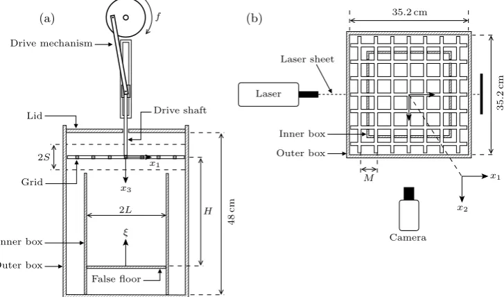
000 000 111 111 0000000000000000 0000000000000000 1111111111111111 1111111111111111 0000 1111 0 0 0 0 0 0 0 0 0 0 0 0 0 0 0 0 0 0 0 0 0 0 1 1 1 1 1 1 1 1 1 1 1 1 1 1 1 1 1 1 1 1 1 1 0 0 0 0 0 0 0 0 0 0 0 0 0 0 0 0 0 0 0 0 0 0 0 1 1 1 1 1 1 1 1 1 1 1 1 1 1 1 1 1 1 1 1 1 1 1 000 000 111 111 (a) (b) 48 cm H 2L ξ f Drive mechanism Drive shaft Grid Lid 2S False floor Inner box Outer box x3 x1 Laser Camera Laser sheet Inner box Outer box M 35.2 cm 35.2 cm x1 x2

Figure 1. Sketches showing the key components of the experimental set-up. (a) A side view showing the positioning of the reciprocating drive mechanism, the horizontal grid, the false floor and the inner and outer boxes. (b) A plan view showing the position of the inner box relative to the grid’s mesh, and the position of the camera relative to the vertical laser-sheet. Also shown are the coordinate directions (x1, x2, x3), and the vertical height normal to the false floor, denoted ξ=H−x3.

2. Experiments

A schematic view of the experimental set-up is shown in figure 1. The experiments were conducted in a transparent acrylic box with internal dimensions 35.2 cm×35.2 cm×50 cm, henceforth denoted the ‘outer box’ (see figure 1). A rigid acrylic lid was suspended horizontally 2 cm below the top of the outer box, which was filled with a salt-water solution of uniform densityρ= 1.028 g/cm3 to the height of the lid’s underside (i.e.the total water depth was 48 cm). The salt used was NaCl. The grid was attached to the base of a stainless steel drive shaft (of 1 cm diameter) and suspended inside the outer box with the plane of the grid horizontal (see figure 1a). The drive shaft passed through a circular hole of 2.6 cm diameter in the centre of the lid. The vertical oscillatory motion of the shaft and grid was driven by using a cam and linear bearing to convert the rotary motion of a motorised flywheel to reciprocating vertical motion of the drive shaft, as shown in figure 1(a). The frequency of the grid oscillation, f, was controlled by using a potentiometer to vary the current across the motor, and was varied between 1.6 Hz and 5.4 Hz. The stroke,S, defined as equal to the amplitude of the grid’s motion, was varied by changing the radius of the flywheel; strokes of S = 2.5 cm and 3.0 cm were used. These ranges for f and S are in line with those used in previous OGT studies (Hopfinger & Linden 1982; Thompson & Turner 1975; Hopfinger & Toly 1976; McDougall 1979; Wan Mohtar & Munro 2013).

M S f(Hz)

(cm) (cm) 1.6 2.2 2.4 2.6 3.1 3.4 3.5 3.8 4.3 4.6 5.4

3.8 2.5 4.1M - 4.1M‡1,

4.9M‡1 - - - 4.1M - - -

-3.8 3.0 - - - - 4.3M - 4.3M,

5.1M - 4.2M - 4.3M

†₄‡₂

5.0 2.5 4.1M†5‡3 4.2M,

4.9M

-4.1M,

4.9M - 4.1M

†₄‡_{4 -} 4.2M,

4.9M - -

-5.0 3.0 - - - 4.2M,

5.0M -

-4.2M,

5.1M 4.3M

Table 1.A summary of the experimental conditions considered. Each entry shows the value of H (relative to the mesh size,M) used for the various combinations ofM,S andf considered. Three of the experiments listed were repeated either n = 4 or 5 times, which are indicated by the†n superscript. In total 31 experiments were performed. A representative subset of the

experiments are used in subsequent sections (to avoid an over saturation of points when plotting data), which we have indicated using the ‡1, ‡2, ‡3, ‡4 superscripts; these four experimental conditions correspond to Reynolds numbers ofReG= 2308 ,6155, 2024 and 4218, respectively.

corresponding mesh spacing (M). This grid type has been widely used in previous OGT studies (Thompson & Turner 1975; Hopfinger & Toly 1976; Hopfinger & Linden 1982; Nokes 1988). The fine grid consisted of a 9×9 array of bars, with square cross-section of 0.6 cm width, and mesh spacingM = 3.8 cm. The corresponding solidities were 36.4% and 28.7% for the coarse and fine grids respectively. The edge conditions of both grids were chosen such that tank sidewalls were planes of symmetry—this condition is known to help reduce the magnitude of secondary flows (De Silva & Fernando 1994).

A small degree of secondary mean flow is inherent in OGT experiments. However, the installation of an open-ended ‘inner box’ has previously been shown to reduce the large-scale circulations that give rise to these secondary flows (Dickinson & Long 1983; Hopfinger & Toly 1976). This approach was adopted here. Two interchangeable inner boxes were used, one for each grid. Each open-ended inner box was fixed centrally on-plan at the base of the tank so that the vertical walls were equidistant between the outermost and second-outermost bars of the grid, as shown in figure 1(b) (for the coarse grid). The grid was then positioned so that when at the bottom of its stoke it was 1 cm above the top of the inner box (see figure 1a). The inner boxes were constructed from 0.5 cm thick transparent acrylic with internal dimensions 24.5 cm×24.5 cm×26.5 cm (for the coarse grid) and 26.1 cm×26.1 cm×26.5 cm (for the fine grid). We will henceforth let 2Ldenote the internal width of the inner box, as shown in figure 1(a). Additional experiments (not reported here) indicated that the inner box reduced, but did not eliminate, the large-scale circulations—a similar effect was reported in the studies by Dickinson & Long (1983) and Hopfinger & Toly (1976). We also stress that the asymmetrical positioning of the grid at the top of the domain did not have a significant effect on the mean flow.

the perimeter of the plate. As a result, the fluid flow between the edge of the plate and the inner tank was negligible.

Here we report results from a total of 31 experiments. Table 1 shows the values ofH used for each combination ofM,S and f considered (see caption for details). The grid Reynolds number (ReG) is defined as

ReG=M Sf /ν; (2.1)

varyingM,S andf as outlined in table 1, corresponded toReG between 1520 and 8100,

which is a relatively broad range in comparison to previous studies using OGT. For example, previous studies of the interaction of OGT with a boundary usedReGbetween

250 and 6660 (Brumley & Jirka 1987; Hannoun et al.1988; Kit et al.1997; McDougall 1979). Further increases in ReG were not possible; proportionately more intense mean

flows (in comparison to the magnitude of the fluctuations) are known to arise at higher grid oscillation frequency (McDougall 1979), such that turbulence produced is a poor approximation to zero-mean-shear turbulence.

Measurements of instantaneous fluid velocities were obtained using two-dimensional particle imaging velocimetry (PIV), applied to the vertical plane through the centre of the grid, in the region inside the inner box spanned by the grid and the false floor. Small, neutrally buoyant tracer particles (Pliolite with diameter range 75 to 125µm) were added to the water volume and thoroughly stirred. A thin light sheet was used to illuminate the particles located within the central, vertical plane. The light sheet was produced by a 100 Hz pulsed laser (Dantec Dynamics NANO L Power 50-100, Class 4). As the grid oscillated, the motion of the illuminated particles, as they were advected by the turbulent flow, was recorded using a high-speed digital camera positioned to point horizontally into the inner tank’s interior, and aligned perpendicular to the plane of the vertical light sheet (see figure 1b). The camera’s capture was synchronised with the pulse of the laser, so the images were recorded at 100 fps (at 1280×1024 pixel resolution). PIV calculations were performed in Digiflow (Dalziel 2006), using square interrogation windows of 13×13 pixels, overlapped to achieve 8 pixel spacing between velocity vectors. This resulted in a physical spacing between velocity vectors of approximately 0.2 cm. Measurements were made only after the grid had been oscillating (at a fixed frequency and stroke) for 15 min to ensure turbulence was fully established. OGT is statistically stationary and so the statistical properties of the flow were analysed using time averages. Hence, in each experiment velocity data were captured for a period of 4 min; analysis of the data showed that the time-averaged mean and rms velocity components were well converged over this period.

The velocity data were calculated and analysed relative to the right-handed coordinate system (x1, x2, x3); here, x3 denotes vertical depth below the mid-height of the grid’s

oscillation, and (x1, x2) are the horizontal coordinates relative to the center of the

grid (see figure 1). The corresponding velocity components are denoted (u1, u2, u3);

the two components measured using the PIV set-up described above are u1(x1, x3, t)

and u3(x1, x3, t), in the central plane at x2 = 0. We use the conventional Reynolds

decomposition ui = Ui +u0i, where u0i(x, t) denote the fluctuating components and

Ui(x) =uithe time-averaged mean components (the overbar notation is used throughout

to denote time averaging). In the calculation of second order quantities, the raw measured values of u1 and u3 were used; we note that calculations of power spectra from time

series at various points within the flow did not indicate the presence of harmonic-like signatures due to grid-forcing in the measured velocity components. We also introduce the coordinateξ=H−x3, which denotes vertical height above the false floor (see figure

stress that all velocities (and derivatives of velocities) were calculated in terms of the right-handed coordinates (x1, x2, x3).

OGT has been used in numerous experimental studies and consistently found to pro-duce turbulence with mean-flow components that are small compared to the fluctuations (McDougall 1979; Hopfinger & Linden 1982; E & Hopfinger 1986; Brumley & Jirka 1987; Fernando & De Silva 1993). For a grid consisting of square bars, the turbulence produced is well described by the standard model

u=C1Sf

x₃

M1/2_S1/2 −γ

, (2.2a)

w=C2u, (2.2b)

`=C3x3, (2.2c)

u0

1u02≈u01u03≈0, (2.2d)

with γ_≈1. In the aboveu≡(u02 1)

1/2_{, v ≡(u}02 2)

1/2_{, w≡(u}02 3)

1/2_{, which are henceforth}

used to denote time-averaged rms velocity components. Symmetry means that u _≈ v is assumed. We stress that the model is only valid for x3 & 2.5M. Previous studies

have shown that the coefficients γ, C1, C2 and C3 are sensitive to the experimental

configuration used, with values typically reported to beγ= 0.8 to 1.5, C1 = 0.2 to 0.5,

C2 = 1.1 to 1.4 and C3 = 0.1 to 0.25 (Thompson & Turner 1975; Hopfinger & Toly

1976; McDougall 1979; Hopfinger & Linden 1982; De Silva & Fernando 1994; Kitet al.

1997; Nokes 1988; Atkinson et al. 1987). The validity of equations (2.2) depends on a number of additional conditions (Fernando & De Silva 1993): the grid solidity should be less than 40%; the grid oscillation frequency should be less than 7 Hz; the grid should be designed to ensure that tank wall’s act as a plane of symmetry. All of these conditions are satisfied with the current apparatus. Data from preliminary testing of the apparatus (forReG between 2050 and 8100), in the absence of the false-floor plate, indicated good

agreement with the standard OGT model (equation 2.2). The spatial structure of OGT of this type is well established and so we omit the presentation of this data here, and instead refer the reader to previous studies for illustrations (see for example Thompson & Turner 1975; Hopfinger & Toly 1976; Kitet al.1997).

3. Turbulence measurements within the bulk interior region

We now describe the turbulence measurements obtained from experiments with the false floor installed. Recall, the floor plate was positioned horizontally at a depth H (between 4M and 5.1M) below the grid’s mean position (see figure 1a). We show in section 4 that the boundary induced effects are mostly confined to a layer of height δs

above the plate, wherein the turbulence is affected by the kinematic blocking condition. At this stage we loosely note that δs is of the order of the integral length scale of the

turbulence; we define this relationship more closely in section 4.2. To begin, however, we first describe the spatial structure of the turbulence within the ‘bulk interior’ of the flow, corresponding to the region above the boundary-affected layer (i.e. ξ_> δs) and below

the near-grid, anisotropic region (i.e.x3>2.5M).

3.1. Sidewall effects

OGT is typically reported to be homogeneous and isotropic in planes parallel to the grid. However, the effect the tank side walls have on the turbulence is not well understood. To assess this effect we consider the degree of isotropy, hw/ui3, across the horizontal

width of the tank, spatially averaged over the vertical direction (between ξ _> δs and

x3>2.5M), whereh·i3is henceforth used to denote the vertical average over this range.

The results obtained are shown in figure 2(a), plotted against the horizontal coordinate x1, which has been scaled by the half-width of the inner box (L). We stress that the data

shown in figure 2(a) are representative of measurements at all depthsx3 within the bulk

interior region and that the spatial averaging, h·i3, has been used here only to reduce

minor scatter. The data indicate a slight dependency on the grid used and so have been shown separately—the solid lines correspond to data obtained using the fine grid, the broken lines to data using the coarse grid (see legend). To avoid over saturation, the data in figure 2(a) are profiles obtained by averaging the results from all the experiments performed for each grid type (12 experiments for the fine grid and 19 experiments for the coarse grid), over the range off andS considered.

To further assess this effect, we also considered the magnitude of the individual rms velocity components across the horizontal width of the tank. That is, the measured rms velocity fields u(x1, x3) and w(x1, x3) were normalised by the corresponding profiles

spatially averaged across the horizontal x1-direction, here denoted by hui1(x3) and

hwi1(x3). A feature of this normalisation is to remove the effects of velocity decay in

thex3-direction. The normalised fields were then spatially averaged in thex3-direction

(i.e.h(u/hui1)i3 andh(w/hwi1)i3) to reduce minor scatter. The normalised rms velocity

components are also shown in 2(a), also averaged over all experiments (by grid type). Figure 2(a) shows that the tank sidewalls have a significant effect, rendering the turbulence anisotropic in regions close to the walls. However, across the central 50% of the tank’s width, the data indicate that the turbulence is approximately isotropic and homogeneous. Hence, throughout the remainder of this paper our attention is focused on this central region and the sidewall (anisotropic) regions are ignored in the calculation of turbulent statistics, so that all spatial averaging in the x1-direction

(denoted h·i1) is henceforth taken over the central 50% region, only. In contrast to the

current results, McDougall (1979) reported significant variations in turbulent velocities across a horizontal plane, even far from the sidewalls. However, the measurements of McDougall (1979) were taken at x3 = 2M, in a region in which jets produced by the

action of the oscillating grid are known to have not fully broken down (Hopfinger & Toly 1976; Atkinsonet al.1987). To our knowledge, the presence of anisotropic sidewall regions has not previously been reported in studies of OGT.

3.2. Degree of isotropy

The horizontally averaged isotropy parameter, hwi1/hui1, is shown in figure 2(b),

plotted against x3/M, and is approximately constant and close to 1 within the bulk

interior region (ξ _> δs, x3 > 2.5M). There is a slight dependency on grid type, and

so the data obtained using the fine and coarse grids are shown separately (see figure caption). For the coarse grid, hwi1/hui1 ≈ 1, however for the fine grid,hwi1/hui1 <1

and slowly tend to 1 as x3 increases. The data do not show any clear dependence on

Reynolds number, ReG. We note that the magnitude of these data are slightly lower

−10 −0.5 0 0.5 1 1

2 3 4

x1/L

0 0.25 0.5 0.75 1 1.25 1.5

1 1.5 2 2.5 3 3.5

hwi1/hui1

x3

/M

(a) h(w/u)i3fine grid (b) h(w/u)i3coarse grid

h(u/hui1)i3fine grid

h(u/hui1)i3coarse grid

h(w/hwi1)i3fine grid

h(w/hwi1)i3coarse grid

ReG= 2308 ReG= 6155 ReG= 2024 ReG= 4218

Figure 2. (a) Normalised profiles hu/hui1i3, hw/hwi1i3 (homogeneity) and the isotropy parameterhw/ui3, each spatially averaged inx3and plotted against the horizontalx1coordinate, which has been scaled by the half-width of the inner box,L. Data obtained using the fine and coarse grids are shown separately (see legend). (b) Measurements of the isotropy parameter

hwi1/hui1 plotted againstx3/M (which, recall, have been spatially averaged across the central 50% of the inner box’s width). The data shown are from the representative subset of experiments (indicated by the‡superscripts in table 1) forReG= 2024, 2308, 4218 and 6155 (see legend).

For each ReG, data from the n repeats are shown, where n = 2, 4 or 5 (see table 1). The

data obtained using the coarse and fine grids are shown separately, indicated by the circles and crosses respectively.

result of excluding the anisotropic sidewall regions in the current results, where the ratio w/uis significantly larger (see figure 2a).

3.3. Spatial decay of the rms velocity components

A defining aspect of OGT is the decrease in magnitude of the rms velocity components with increasing depth below the grid. In section 2 we noted that in the absence of the floor plate the measured rms velocity components are well described by the standard model (2.2). With the plate inserted, the measurements of uand wexhibited a similar spatial decay away from the grid and so again we sought to fit to the data power laws of the form

u=CuSf

x₃

M1/2_S1/2 −γu

, (3.1a)

w=CwSf

x₃

M1/2_S1/2 −γw

, (3.1b)

in the bulk interior regionξ_>δs,x3>2.5M. For each experiment a single value of each

of the coefficientsCu,Cw, and exponentsγu,γw were obtained using a regression best

fit. Figure 3(a) shows typical examples of the regressions fits applied to measurements of the rms velocity componentu; the results are shown for four separate experiments, but performed under nominally identical conditions with ReG = 4218. The goodness of fit

and degree of scatter evident for these data are representative of all the experiments. A similar goodness of fit (and scatter) were found for the vertical rms velocity component (w). The fitted values ofγuand γw, for each of the 31 experiments, are shown in figure

3(b), plotted against corresponding Reynolds numberReG. Figure 3(b) indicates that the

fitted decay exponents exhibit significant departure in magnitude relative to the idealised model (γu=γw= 1), with no apparent dependence onReG; this effect is most notable for

3.5 4 4.5 5 5.5 0.08

0.09 0.1 0.11 0.12 0.13

x3/M

1/2

S1/2

h

u

i1

/f

S

1000 3000 5000 7000 9000

−0.5 0 0.5 1 1.5 2

ReG

γu

,

γw

(a) (b) Coarse grid,u

Coarse grid,w Fine grid,u Fine grid,w

Figure 3.Plots showing the results of fitting the decay laws in equation (3.1) to the experimental data. (a) Measurements of u(crosses) compared with the corresponding regression best fit of equation (3.1a) (broken lines). The results are shown from four separate experiments, but each performed under nominally identical conditions withReG= 4218. The fits were performed in the

bulk interior region (withx3>2.5M andξ > δs). For comparison, a decay exponent equal to 1

is also shown, by the solid line. (b) The fitted exponentsγu,γwfrom each of the 31 experiments,

plotted against grid Reynolds numberReG.

in figure 3(b) show that repeating experiments under nominally identical conditions can result in variations in the resulting decay exponent. This is not unexpected; for example, (McKenna & McGillis 2004) showed that the magnitude of turbulent fluctuations may vary by as much as 15% from separate experiments performed under the same conditions.

3.4. Mean flow

The mean flow is an integral aspect of OGT and, as noted in section 2, the presence of the inner box reduced but did not eliminate the large circulations that give rise to the mean flow. The mean flow within OGT has been studied in detail in numerous previous studies (see for example De Silva & Fernando 1994; McKenna & McGillis 2004; McDougall 1979; Dohan & Sutherland 2002), and the qualitative characteristics of the mean flow observed with our apparatus are little different to those reported in these studies. In particular, the mean flow is not symmetrical, being most intense close to the grid (and tank walls) and decaying with distance below the grid. Plots showing typical mean-flow fields observed in OGT can be found, for example, in McKenna & McGillis (2004).

The effect the presence of the floor plate had on the magnitude of the secondary flow was assessed using the inverse turbulence intensities h|U1|/ui1 and h|U3|/wi1 (as

previously used by Variano & Cowen 2008), which are shown in figure 4 plotted against scaled height ξ/δs above the plate. Recall thatδs denotes a thin layer adjacent to the

plate in which the boundary induced effects, on the turbulence statistics, are mostly confined within. As the plate surface at ξ = 0 is approached, the vertical intensity h|U3|/wi1 is reduced towards zero, whereas the horizontal intensity h|U1|/ui1 typically

exhibits an increase to a peak value, before reducing at the boundary. Note that figure 4 indicates that the measured intensities h|U1|/ui1 and h|U3|/wi1 show no apparent

dependence onReG, over the range ofReG considered. Most importantly, figure 4 shows

0 0.25 0.5 0.75 1 1.25 1.5 0

1 2 3 4

h(|U1|/u)i1

ξ

/

δs

0 0.25 0.5 0.75 1

0 1 2 3 4

h(|U3|/w)i1

ξ

/

δs

(a) ReG= 2308 (b)

ReG= 6155 ReG= 2024 ReG= 4218

Figure 4. Plots showing the inverse turbulence intensities h|U1|/ui1 and h|U3|/wi1 plotted against height above the plate ξ, which has been scaled by the δs, the thickness of the

boundary-affected region. The data shown are from the representative subset of experiments (indicated by the‡superscripts in table 1) forReG= 2024, 2308, 4218 and 6155 [see legend in

(a)]. For eachReG, data from thenrepeats are shown, wheren= 2, 4 or 5 (see table 1).

to allow meaningful comparisons to be made with previous studies based on zero-mean-shear conditions. The small levels of mean-zero-mean-shear do result in production of TKE, although we will show in section 5.2 that the level of production is small.

4. Turbulence measurements in the boundary-affected region

We now focus attention on describing the turbulence characteristics (integral length scale and rms velocity components) in the boundary-affected region and compare our results to those available within the literature. The mechanisms that give rise to these results are explored in the subsequent sections.

4.1. Integral length scales

Estimates for integral length scales were obtained from the velocity measurements by computation of autocorrelation coefficients. We followed the approach used previously by Kitet al.(1997) by defining the integral length scale as the integral of the autocorrelation function ofu0₁(x1, x3, t), over the spatial lag up to which the autocorrelation function first

crosses zero. The autocorrelation function, at spatial lagχ, is defined as

ru(x3, t;χ) =

cu(x3, t;χ)

cu(x3, t;χ= 0)

, (4.1a)

where

cu(x3, t;χ) =

1 L

Z L/2

−L/2

u0₁(x1, x3, t)u01(x1+χ, x3, t) dx1. (4.1b)

Recall,Ldenotes the half-width of the inner box. The time-averaged integral length scale is then given by

`(x3) =

1 T

Z T

0 Z χ0

0

ru(x3, t;χ) dχdt (4.2)

whereχ0denotes the spatial lag at which the autocorrelation function first becomes zero,

1 1.5 2 2.5 3 3.5 4 0

2 4 6 8

ℓ(cm)

ξ

(c

m

)

0 0.25 0.5 0.75 1 1.25

0 0.5 1 1.5 2 2.5

ℓ/ℓ0

ξ

/ℓ

0

(a) ReG= 2308 (b)

ReG= 6155

ReG= 2024

ReG= 4218

Hunt and Graham (1978) Thomas and Hancock (1977)

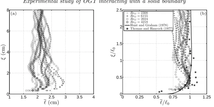
Figure 5. (a) Computed values of the time-averaged integral length scale,`, plotted against height ξ. (b) The same data but scaled by the reference integral length scale, `0, from each experiment. The data obtained using the coarse and fine grids are shown separately, indicated by the circles and crosses, respectively. The data shown are from the representative subset of experiments (indicated by the ‡superscripts in table 1) forReG= 2024, 2308, 4218 and 6155

[see legend in (b)]. For each ReG, data from the n repeats are shown, where n = 2, 4 or 5

(see table 1). Also shown in (b) are corresponding experimental data from Thomas & Hancock (1977) and a prediction based on RDT by Hunt & Graham (1978) (see legend).

In previous studies of the interaction of zero-mean-shear turbulence with a boundary, a reference length scale`0 has been used (Hunt & Graham 1978; Perot & Moin 1995).

In these studies the turbulence beyond a boundary-affected region is homogeneous with a corresponding constant value of integral length scale, and so naturally this far-field integral length scale was used for`0. The situation is potentially more complex for OGT,

as the integral length scale ` is expected to depend on x3 in the far-field. Figure 5(a)

shows the computed values of`obtained from the current data, which are plotted against height,ξ, above the plate. Beyond the boundary-affected region, forξ >3 cm, the data for `are relatively constant, taking values between 2 cm and 2.5 cm, but exhibit a significant degree of scatter. The data at heightsξ <3 cm, increase slightly, before rapidly reducing at ξ≈0.75 cm. The level of scatter in the data made it difficult to identify a trend for ξ >3 cm. Hence, the approach taken here was to define the reference integral length scale `0 to be the peak value attained by` (in the near-boundary region). This length scale

remains physically intuitive; at this distance from the boundary the maximum integral eddy size first feels the effect of the wall. No link between the magnitude of`0 (or`) and

Reynolds numberReG was observed.

We can more clearly consider the effect of the boundary on the integral length scales by considering the data shown in figure 5(b), of `/`0plotted against scaled heightξ/`0.

For ξ < `0 integral length scales increase to a maximum, before reducing rapidly as

the boundary is approached. However, the level of increase in `/`0 varies significantly

between experiments and appears slightly larger for the fine grid than the coarse grid and so the data obtained using the coarse and fine grids are shown separately (see figure caption for details). A slight increase in` was also reported in the results of Thomas & Hancock (1977), and these data are also shown in Figure 5(b) (see legend).

Figure 6(a) shows corresponding measurements of the time-averaged transverse integral length scale,`w, which were obtained using equation (4.2), withrwused in place ofru,

which is defined using equation (4.1) with u0₃ in place of u0₁. In figure 6(a),`w is scaled

0 0.25 0.5 0.75 1 0

0.5 1 1.5 2 2.5

ℓw/ℓ

ξ

/ℓ

0

0 0.25 0.5 0.75 1 1.25 1.5

0 0.5 1 1.5 2 2.5

hwi1/hui1

ξ

/ℓ

0

(a) (b)

ReG= 2308

ReG= 6155

ReG= 2024

ReG= 4218 Hunt and Graham (1978) Kit et al. (1997) Thomas and Hancock (1977)

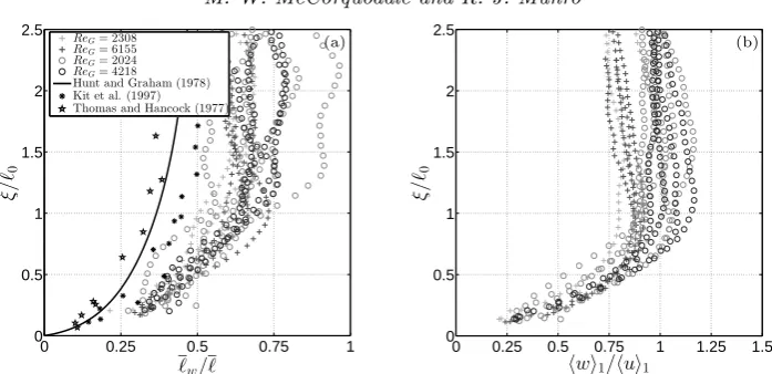
Figure 6.(a) Computed values of the time-averaged transverse integral length scale,`w, scaled

by`and plotted against scaled heightξ/`0. Also shown are corresponding experimental data from Thomas & Hancock (1977) and Kitet al.(1997), and a prediction based on RDT by Hunt & Graham (1978) (see legend). (b) Measurements of the degree of isotropyhwi1/hui1, plotted against normalised height ξ/`0. The data obtained using the coarse and fine grids are shown separately, indicated by the circles and crosses, respectively. In both plots the data shown are from the representative subset of experiments (indicated by the ‡superscripts in table 1) for ReG= 2024, 2308, 4218 and 6155 [see legend in (a)]. For eachReG, data from thenrepeats are

shown, wheren= 2, 4 or 5 (see table 1).

quasi-isotropic turbulence; recall that for isotropic turbulence `w/`= 0.5 (Pope 2000).

`w deviates from its far field value atξ≈`0, initially appearing to reduce to zero at the

boundary in line with the prediction of inviscid RDT analysis of Hunt & Graham (1978) and in approximate agreement with the results of Thomas & Hancock (1977) and Kit

et al.(1997) which are also shown in figure 6 (see legend). This reduction is expected at a solid boundary; at a distanceξ < `0from the boundary, eddies of size greater thanξwill

have been blocked, such that remaining eddies are of wavenumberkw> ξ−1. Note that

the rapid reduction inlwwithin the boundary-affected region as a result of the blocking

condition renders the integral length scales anisotropic. In addition, figures 5 and 6(a) indicate that both`/`0and`w/`are independent of Reynolds number, over the Reynolds

number range considered.

4.2. RMS velocity data

Measured values of the degree of isotropy are shown in figure 6(b), plotted against scaled height ξ/`0. We note there is no apparent dependence on Reynolds number,

ReG, but there is a slight dependence on the grid type used, and so the data obtained

using coarse and fine grids are shown separately (see figure caption for details). These data can be used as an indicator of the thickness of the boundary-affected region by noting the point at which values deviate from those in the far-field. Figure 6(b) shows a rapid increase in anisotropy occurs at ξ/`0 ≈ 1, departing from the far-field trend. This is in accordance with the results of the integral length scales shown in figures 5 and 6(a). We therefore conclude that the boundary-affected region extends up to ξ/`0≈1, and henceforth throughout the remainder of this paper assume that the boundary-affected region has thickness δs = `0. We also note that the grid Reynolds number

0 0.25 0.5 0.75 1 1.25 0

0.5 1 1.5 2 2.5

hwi1/w0

ξ

/ℓ

0

0.50 0.75 1 1.25 1.5

0.5 1 1.5 2 2.5

hui1/u0

ξ

/ℓ

0

(a) (b)

ReG= 2308

ReG= 6155

ReG= 2024

ReG= 4218 Hunt and Graham (1978) Hunt (1984) Aronson et al. (1997) Hannuon et al. (1988) Kit et al. (1997) Thomas and Hancock (1977) Brumley and Jirka (1987)

0 0.5 1 1.5 2

1 1.1 1.2 1.3 1.4 1.5 1.6

γu

m

ax

(

h

u

i1

/u

0

)

0.50 0.75 1 1.25 1.5

0.5 1 1.5 2 2.5

hui1/u0_,ℓ0

ξ

/ℓ

0

(c) ReG= 2308 (d)

ReG= 6155

ReG= 2024

ReG= 4218 Bodart et al. (2010) McDougall (1979) Fine grid

Coarse grid

Figure 7.(a,b) Plots showing the scaled rms velocity componentshwi1/w0andhui1/u0, plotted

against scaled heightξ/`0. The data shown are from the representative subset of experiments (indicated by the ‡ superscripts in table 1) for ReG= 2024, 2308, 4218 and 6155 [see legend

in (a), which applies to both plots]. For each ReG, data from then repeats are shown, where

n = 2, 4 or 5 (see table 1). Also shown are corresponding experimental data (Aronsonet al.

1997; Hannounet al.1988; Kitet al.1997; Thomas & Hancock 1977; Brumley & Jirka 1987) and predictions based on RDT (Hunt & Graham 1978; Hunt 1984) (see legend). (c) Plot showing max(hui1/u0) for each experiment, plotted against decay exponent γu (from equation 3.1a).

Data are shown for all 31 experiments, with the data obtained using the coarse and fine grids shown separately [see legend]. (d) Measurements of the rms velocity component hui1, plotted against scaled heightξ/`0. In this case,hui1 has been normalised by the value ofu0 evaluated at ξ=`0, denotedu0,`0. The data shown are from the representative subset of experiments, with ReG= 2024, 2308, 4218 and 6155 (see legend). Also shown are corresponding experimental data

from McDougall (1979) and results of simulations by Bodartet al.(2010) (see legend).

In order to consider the effect of the boundary on the rms velocity components for ξ < δs(recalling that forξ > δs,uandwdecay with increasingx3), we normalise results

by corresponding values we would expect in the absence of the boundary. The expected values were determined from best fits of the power laws in equation (3.1), denoted byu0

andw0, applied to the measurements ofhui1andhwi1in the region above the

boundary-affected layer, ξ > δs (shown in figure 3a). This method of normalisation is similar to

component (w), shown in figure 7(a), we observe a monotonic reduction of the normalised velocity as the boundary is approached, which is independent of Reynolds number. Quantitative agreement is obtained with a range of studies (see legend) investigating the interaction of zero-mean-shear turbulence (Hunt & Graham 1978; Hannoun et al.

1988; Kitet al. 1997; Thomas & Hancock 1977; Brumley & Jirka 1987). We stress that these previous studies cover a range of boundary types (density interface, free surface and solid boundary) and are for turbulence that is homogeneous beyond the boundary-affected region, as well as for spatially decaying turbulence.

In contrast, measurements of the boundary-tangential component (u), shown in Figure 7(b), exhibit a greater level of scatter and provide a lesser degree of quantitative agreement with previous studies. In the current results values of u were amplified within the boundary-affected region, attaining a maximum atξ/`0≈0.25 before rapidly reducing as ξ→0. Results show qualitative agreement with a range of studies utilising turbulence that spatially decays in thex3direction (Hannounet al.1988; Kitet al.1997;

Brumley & Jirka 1987). In contrast, although the RDT proposed by Hunt & Graham (1978) predicts amplification of the velocity component outside the viscous sub-layer, RDT under-predicts the amplification observed. The modified RDT proposed by Hunt (1984) provides a better approximation of the amplification observed for the coarse grid. Poor agreement is obtained with the study of Aronsonet al.(1997). However, the results of Aronson et al.(1997) and Thomas & Hancock (1977) were obtained from studies in which turbulence was homogeneous beyond the boundary-affected region. The results of Thomas & Hancock (1977) display features similar to the current results, however, we note their results have been questioned in light of frictional heating of the apparatus (Aronsonet al. 1997).

We stress that the amplification of hui1/u0 does not exhibit a clear dependence on

Reynolds number, instead figure 7(c) shows that the maximum amplification ofhui1/u0

is weakly correlated with the decay rate of the velocity componentγu, which may mask

any Reynolds number effects, over the fairly narrow range of Reynolds number considered here. This is an important point and goes some way to address the disparity in results previously reported in the literature. Specifically, the previous studies that have identified u/u061 are for the case where the far-field turbulence is homogeneous (Aronsonet al.

1997; Perot & Moin 1995), which correspond to the case γu = γw = 0. In contrast,

a number of studies that have predicted u/u0 > 1 for ξ < δs are for the case of

inhomogeneous far-field turbulence, with γu, γw 6= 0 (Hannoun et al. 1988; Kit et al.

1997; Brumley & Jirka 1987). As such, this data suggests that the trend of u/u0 for

ξ < δs depends crucially on the nature of the turbulence itself (homogeneous versus

inhomogeneous); this effect is considered further in section 5. Note that there is a clear grid-dependence in the data shown in figure 7(c), which can be understood by noting that the rate of spatial decay of rms velocity was lower in experiments using the fine grid than the coarse grid (see section 3.3 and figure 3b).

In addition to the data normalisation described above using u0 and w0, it is also

informative to consider the measurements of hui1 scaled by the characteristic value

of u0 at the edge of the boundary-affected region, at ξ = `0, henceforth denoted

u0,`0. Figure 7(d) shows the measurements of hui1 scaled by u0,`0, which indicate that,

on average, hui1/u0,`0 & 1 in the region for ξ < `0, before rapidly reducing as the

region isδs≈`0≈0.36lf (based on their figure 3b), wherelf denotes the characteristic

length scale used by Bodartet al.(2010). Constant values ofuin the boundary-affected region were also obtained in the results of McDougall (1979), which are also shown in figure 7(d) (see legend). Note however that given that both the studies of Bodartet al.

(2010) and McDougall (1979) featureudecaying spatially with increasing distance normal to the source (in our notation, the x3-direction), a tendency for uto attain a constant

value in the boundary-affected region implies thatuis amplified relative to the far-field trend. Hence, the results from these studies are in agreement with our results shown in 7(b), but opposed to the results of Aronsonet al.(1997) and Perot & Moin (1995) from homogeneous turbulence.

5. Turbulent kinetic energy in the boundary-affected region

We have established that, in the current experiments,hui1/u0 >1 (such that hui1&

u0,`0) andhwi1/w0<1 in the boundary-affected region. It is tempting to attribute these

results to inter-component energy transfer from the w2 _{component to u}2 _component.

However, measurements of TKE, here defined as q02 _{= u}0

iu0i/2 ≈ (2u01u01 +u03u03)/2

(assumingv_≈u), are shown in figure 8, plotted against scale heightξ/`0. Two methods

of normalisation have been used: figure 8(a) shows hq02_i

1 scaled by q002, which denotes

the trend expected in the absence of the boundary, obtained from a best fit applied to the data above the boundary-affected region; figure 8(b) shows hq02_i

1 scaled by q0₀2_,`0,

which denotes the value of q02

0 evaluated at the edge of the boundary-affected region, at

ξ = `0. Crucially, figure 8(a) shows that the values of hui1/u0 > 1 observed in figure

7(b) cannot be due only to intercomponent energy redistribution since there is also an increase in TKE within the boundary-affected region relative to the far-field trend. Figure 8(b) shows that on average TKE is in fact approximately constant across the boundary affected region, but that for some experimentshq02_i

1/q002,`0 >1. Figure 8 also shows that

there is no clear Reynolds number dependency in the data, instead indicating that the TKE is typically higher in the data obtained using the coarse grid, compared to that obtained with the fine grid, which are shown separately (see figure caption for details).

A likely contributory factor to the increase in TKE is a net production or advection of TKE in this region by the mean flow (which is shown to be the case in section 5.2 below), however the small levels of mean flow typically present in OGT suggest that another mechanism may be, at least partially, responsible for this result. We therefore consider the vertical flux of TKE produced by the oscillation of the grid. Measurements of the vertical flux of TKE,hu0

3q02i1, are shown in figure 9(a), plotted against scaled height

ξ/`0. The data have been scaled by their expected values in the absence of the boundary,

denoted (u0

3q02)0, obtained by finding a best fit of the formhu03q02i1∝x−

γ

3 applied to the

data above the boundary-affected region. This normalisation is in line with the method used in section 4.2. Under idealised conditions one would expect γ= 3; however, given the deviations inγuandγwfrom 1, the average of the fitted values forγwas 2.4. Hannoun

et al.(1988) applied a similar method and reportedhu0₃q02_i1/3_/u

≈constant.

The data in figure 9(a) show a significant reduction in energy flux in the boundary-affected region (ξ/`0<1) relative to the far-field trend and are in good agreement with

0.250 0.5 0.75 1 1.25 1.5 1.75 0.5

1 1.5 2 2.5

hq′2_i 1/q′

2 0

ξ

/ℓ

0

0.4 0.6 0.8 1 1.2 1.4

0 0.5 1 1.5 2 2.5

hq′2

i1/q′02_,ℓ0

ξ

/ℓ

0

(a) (b)

ReG= 2308

ReG= 6155

ReG= 2024

ReG= 4218

Hannoun et al. (1988)

Figure 8.(a) Measurements of TKEhq02_i

1, plotted against scaled heightξ/`0. Here,hq02i1 has been normalised by the decay q02

0 based on the far-field trend. (b) Shows the same data but withhq02_i

1 scaled by the value ofq002 at the heightξ/`0= 1, denotedq002,`0. The data shown are from the representative subset of experiments (indicated by the ‡superscripts in table 1) for ReG= 2024, 2308, 4218 and 6155 [see legend in (a), which applies to both plots]. For eachReG,

data from thenrepeats are shown, wheren= 2, 4 or 5 (see table 1). Also shown are data taken from Hannounet al.(1988).

the cause of the amplified TKE measured in this region. The current results support this interpretation and indicate that this effect contributes to the observed values of hq02_i

1/q002>1. However, the increase inhq02i1/q002,`0 >1 cannot be explained by turbulent

transport, since in isolation the vertical flux of kinetic energy by turbulent transport would result inhq02_i

1≈q002,`0; values ofhq 02_i

1/q002,`0 >1 would cause re-adjustment of the

flow beyond the boundary-affected region and an increase inq02

0. We stress that this effect

is not a Reynolds number effect. Instead, in section 5.2 we show there is a significant increase in advection of u2 _{by the mean flow into the central region of the tank for}

ξ/`0<0.3, and that this is a major contributing factor to the increase in TKE over this

region.

To better understand the vertical flux of TKE in the boundary-affected region we have decomposedhu0₃q02_i

1into its component hu03u012i1,hu033i1 and in figure 9(b) plotted

the correlation coefficients hu0

3u012i1/hwu2i1 andhu033i1/hw3i1 against scaled heightξ/`0.

We note that, as far as we are aware, these measurements are the first reported of this type for OGT. In figure 9(b) the notation hu0

iu0iu03i1/hwu0i2i1 has been used (with the

summation convention dropped) so that the correlation coefficients are given by i = 1 andi= 3. To avoid oversaturation, the data shown are from only three Reynolds numbers (ReG = 2024, 4218 and 6153) and each data profile (see figure legend) is an average of

measurements taken from four (or five) repeated experiments performed under each of these conditions (see table 1 for details).

The correlation coefficienthu03

3i1/hw3i1 of the vertical flux ofw2—which is the

−10 −0.5 0 0.5 1 1.5 2 0.5

1 1.5 2 2.5

hu′

3q′2i1/(u′3q′2)0

ξ

/ℓ0

−0.250 0 0.25 0.5 0.75 1 1.25

0.5 1 1.5 2

hu′

iu′iu′3i1/hwu′_i2i1

ξ

/ℓ

0

(a) (b)

ReG= 2308

ReG= 6155

ReG= 2024

ReG= 4218

Hannoun et al. (1988)

i= 1, ReG= 2024

i= 1, ReG= 4218

i= 1, ReG= 6155

i= 3, ReG= 2024

i= 3, ReG= 4218

i= 3, ReG= 6155

Figure 9.(a) Measurements of the vertical flux of TKE,hu03q02i1, plotted against scaled height ξ/`0. The data have been normalised by the trend expected in the absence of the floor plate, denoted (u0

3q02)0. The data shown are from the representative subset of experiments (indicated by the‡superscripts in table 1) forReG= 2024, 2308, 4218 and 6155 (see legend). For eachReG,

data from thenrepeats are shown, wheren= 2, 4 or 5 (see table 1). Also shown are data taken from Hannounet al.(1988). (b) Measurements of correlation coefficientshu0

iu0iu03i1/hwu0i2i1 for i= 1 andi= 3 (with the summation convention dropped), plotted against scaled height ξ/`0. The data are shown are from the representative subset of experiments, forReG = 2024, 4218

and 6155 (see legend).

energy of turbulent motions away from the boundary. There are two possible effects that could lead to a relative depletion of energy from the vertical component of the turbulent motions away from the plate. (i) It is possible that there is a net intercomponent energy transfer from w2 _{to u}2 _{at the boundary. (ii) Alternatively, it is possible that energy}

of turbulent motions near the boundary is depleted by viscous effects (splat-antisplat imbalance). In isolation it is not possible to determine which effect is prevalent in this case.

The correlation coefficient hu0₃u02

1i1/wu2, of the vertical flux of u2, is shown in figure

9(b) (by the solid lines), and is also positive far from the boundary, indicating a flux of energy away from the grid. In contrast to the vertical flux of w2, on approach to the boundary the vertical flux ofu2 is small but becomes negative, indicating that there is a small net flux ofu2_{away from the boundary associated with antisplats. In light of the flux}

ofw2_{, the negative flux ofu}2 _{appears to suggest that the effect (i) (above) is prevalent}

at the boundary, such that antisplats have greater horizontal velocities than splats in the near-wall region as a result of intercomponent energy transfer. However, recall that over this region there was also an increase in hq02_i

1/q002,`0, shown in figure 8(b), due to

advection by the mean flow; this is a major contributing cause to the more energetic antisplats found in the current results. Hence, it appears that the small upwards flux of u2_{observed forξ <0.5`}

0here is not necessarily a result of (i), but is actually a result of a

departure from the zero-mean-shear condition. Recall also that in this regionu > w(see figure 6b). Hence, as the boundary is approached the vertical flux of TKE is dominated by trends in the vertical flux ofu02

1. Hence, it is this reversing orientation of vertical flux

ofhu0

3u012i1that results in the small upwards flux ofhu03q02i1 close to the boundary.

Overall, as a result of the blocking of the vertical flux of TKE we observe a net flux of energy into the boundary-affected region. This results in values hui1/u0>1 without

otherwise arise in the region occupied by the boundary is halted. This will constitute a major factor in the difference in results of u/u0 and w/w0 reported in the studies

of Aronson et al. (1997) and Perot & Moin (1995) when compared to studies utilising OGT; these studies represent fundamentally different conditions. Although we have not considered the transport of TKE by viscous or pressure effects here, they are considered in section 5.2 below and do not invalidate the previous conclusions.

5.2. Reynolds stress and turbulent kinetic energy balances

The steady form of the Reynolds stress transport equations may be written as (see Hinze 1975, p. 323)

0 =−Uk

∂ ∂xk

u0

iu0j

| {z }

Ad ij

−u0

ju0k

∂Ui

∂xk −u0

iu0k

∂Uj

∂xk

| {z }

Φij

− ∂ ∂xk

u0

iu0ju0k

| {z }

Tij

−1 ρ

_∂

∂xi

p0_u0

j+

∂ ∂xj

p0_u0

i

| {z }

Πd ij +1 ρp 0 _∂u0 j ∂xi + ∂u 0 i ∂xj

| {z }

Πs ij

+ν ∂

2_u0

iu0j

∂xk∂xk

| {z }

Dij

−2ν∂u

0

i

∂xk

∂u0_j ∂xk

| {z }

εij

. (5.1)

The termsAd

ij and Φij denote, respectively, transport and production due to the mean

flow;TijandΠijd denote, respectively, transport by velocity and pressure fluctuations;Π s ij

is the inter-component energy redistribution due to the correlation between fluctuating strain and pressure fields;Dij andεij denote molecular diffusion and viscous dissipation.

Recall that within the inner box’s central region—the region of interest—the turbulence is approximately homogeneous on horizontal planes and so u0

iu0j ≈0 for i 6=j. Hence,

we only consider the transport equations for the Reynolds stressesu0₁u0₁,u₂0u0₂andu0₃u0₃ (i.e. u2_{, v}2 _{and w}2_{), and the transport equation for TKE which is obtained from the}

trace of (5.1) noting that u0_iu0_i/2 = q02 _{denotes the TKE. We note that, as far as we}

are aware, the current results are the first attempt to evaluate (5.1) using data obtained from OGT.

A direct evaluation of (5.1) was not possible, requiring instantaneous measurements of pressure fluctuations and of all three velocity components. Hence, a number of simplifying assumptions were made to allow estimation of certain terms: (i) Based on the symmetry of the experimental set-up, the time-averaged statistical properties of the flow were assumed to be symmetric in the x1- and x2-directions. (ii) The turbulence was assumed to be

approximately homogeneous in horizontal planes. (iii) The approximations (∂u0₁/∂x2) 2

≈ 2(∂u0₁/∂x1)

2

and (∂u0₃/∂x2) 2

≈(∂u03/∂x1) 2

were used in calculation of the dissipation terms—relationships which are known to hold for homogeneous, isotropic turbulence (see Pope 2000, p. 134). Under these assumptions, the relevant terms in (5.1) involving velocity components (and derivatives of velocity components) were calculated from the 2D PIV data obtained in the central (x1, x3)-plane. When evaluating the velocity derivatives, the

no slip and impermeability conditions (ui = 0) were applied at ξ = 0. We note that

limitations in the resolution of the PIV method (a resolution of approximately 0.2 cm) is insufficient to capture all scales of turbulent motion and may lead to underestimation of some terms (primarily the diffusionDij and dissipationεij terms) in equation 5.1.

It was not possible to directly estimate the terms Πs

ij and Πijd involving pressure

fluctuations. These terms were instead estimated from a balance of the remaining terms in (5.1), the approach used previously by Aronsonet al.(1997). Firstly, noting thatΠs

ii = 0

equation (5.1) fori=j. Secondly, using the property that the turbulence is approximately homogeneous in horizontal planes means that Πd

11 ≈ Π22d ≈ 0 and Πiid ≈ Π33d , which

enables estimation ofΠs

11 andΠ33s from the equations (5.1) foru01u01 andu03u03.

The scheme outlined above inevitably produced significant scatter in the results. In an effort to reduce scatter we show here the results for three experimental conditions, with ReG = 2024, 4218 and 6155 (spanning the range of Reynolds numbers considered

here). Each experiment was repeated four (or five) times (see table 1) and the results obtained from each were averaged, which are shown in figure 10, plotted against scaled height ξ/`0. Note also that the data shown are averaged in the x1-direction (i.e.h·i1).

In figure 10 the left-hand column of data show terms from the TKE budget equation (u0

iu0i), while the central and right-hand columns of data show the terms from theu

2_and

w2 _{budgets. To facilitate comparison, the data have been normalised by the magnitude}

of the corresponding component of energy dissipation evaluated at the height ξ = `0

(denoted |εii|`0, |ε11|`0, |ε33|`0 in the caption and figure labels). The top, second and

third row of data in figure 10 are for ReG = 2024, 4218 and 6155, respectively. We now

consider separately the data for the budgets for TKE,u2_andw2_.

Terms of the TKE budget

The terms for the TKE budget are shown in figure 10(a-c), at the three Reynolds numbers. Within the boundary-affected region (ξ/`0 <1), but for ξ/`0>0.3, the data

show that the budget is dominated by comparatively high levels of turbulent transport (Tii). Over this regionTii increases in magnitude, indicating a source of energy in this

region. This is a direct result of the blocking of vertical energy flux—note thatTiiis the

derivative of TKE flux previously considered in section 5.1. Across this region dissipation (εii) is approximately constant. Hence, it appears that the increase inTii is the primary

cause of the increase inhq02_i

1/q002observed over the region 0.3< ξ/`0<1, shown in figure

8(a). In contrast, forξ/`0<0.3 the data shows thatTii clearly reduces to approximately

zero as the energy flux close to the wall is approximately zero. As a consequence, turbulent transport no longer acts as a source of energy in this near-boundary region.

Within the boundary-affected region we also observe an increase inΠd

ii forξ/`0<0.3,

and at the higher two Reynolds numbers the data exhibit a distinct peak before reducing as the boundary is approached. The results forΠd

iishow good qualitative agreement with

data reported in the previous studies by Bodartet al.(2010) and Perot & Moin (1995). The profile ofΠd

iiacross the boundary-affected region indicates that higher instantaneous

pressure is correlated with turbulent fluctuations incident towards the boundary; that is, here the turbulence is homogeneous only in planes parallel to the grid, and soΠ_iid =Π₃₃d (note that in figure 10, the magnitudes ofΠ_iid andΠ33d are not the same as they have been

normalised differently, by|εii|`0 and|ε11|`0, respectively). This correlation between high

pressure events and fluid elements incident towards the boundary can be understood by considering that splats are more energetic than antisplats, so result in a greater instantaneous pressure. For ξ/`0 . 0.2, the data for Πiid reduces as the transport of

pressure fluctuations by the turbulent velocity must tend to zero at the limit of the wall. The data for dissipation of TKE (εii) show that TKE is lost throughout the domain

(due to deformation work done by viscous stresses). Previous studies (using DNS) have suggested that TKE dissipation increases significantly as the boundary is approached (Bodart et al. 2010; Perot & Moin 1995), however, the PIV data reported here did not resolve scales sufficiently close to the boundary to validate this proposal. In addition, figure 10 indicates that the transport of turbulent kinetic energy by viscous diffusion (Dii)

is negligible beyond the viscous sublayer (ξ/`0>0.3). However, in previous studiesDii