Magnetic resonance elastography

Magnetic Resonance Elastography

Deirdre M. McGrath

Table of Contents

1. Overview of Elasticity Imaging

2. Categories of Magnetic Resonance Elastography

3. Comparison of Magnetic Resonance Elastography with Alternative Methods 3.1 Conventional Medical Imaging

3.2 Manual Palpation

3.3 Alternative Elasticity Imaging Methods 4. Background of Magnetic Resonance Imaging 5. Magnetic Resonance Elastography Methodology

5.1 Dynamic MRE

5.1.1 Dynamic MRE Hardware 5.1.2 Dynamic MRE Pulse Sequences 5.1.3 Dynamic MRE Inversion Methods

5.1.3.1 Direct Inversion

5.1.3.2 Local Frequency Estimation

5.2.1 Quasi-static MRE Hardware 5.2.2 Quasi-static MRE Pulse Sequences 5.2.3 Quasi-static MRE Inversion Methods

5.2.3.1 Direct Inversion

5.2.3.2 Iterative Finite Element Model Based Inversion 6. Applications of Magnetic Resonance Elastography

6.1 Clinical Applications 6.1.1 Liver

6.1.2 Spleen and Kidneys 6.1.3 Brain

6.1.4 Prostate 6.1.5 Breast

6.1.6 Musculoskeletal 6.2 Pre-clinical Applications 7 Future Challenges

8 Conclusions

Magnetic resonance elastography (MRE) is a recently developed technology that uses MRI to measure the biomechanical properties of biological tissue, such as elasticity and viscosity. Due to its sensitivity to pathology-driven alterations in tissue biomechanics, MRE is a powerful

The technology is undergoing rapid development for application to multiple organ sites in the body, and is already widely adopted in clinical practice for diagnosing hepatic fibrosis. This chapter will provide an overview of the background, methodology and clinical applications of MRE.

1. Overview of Elasticity Imaging

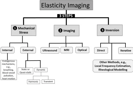
MRE methods fall within the broader general classification of elastography or elasticity imaging, which includes non-MRI based methods. Elasticity imaging consists of three steps: 1) generation of a mechanical stress within the biological tissue, which could be the result of an applied

external mechanical force, or an internal endogenous mechanism (e.g., breathing, heart motion, or blood vessel pulsation); 2) observation of the strain response (e.g., displacement field or velocity) via an imaging method such as MRI, ultrasound or optical imaging; 3) application of an inversion algorithm to calculate biomechanical properties from the observed stress-strain

dynamics (Figure 1).

() is usually estimated as that of water (1000 kg/m3_{). While some tissue types can be} approximated as a material with isotropic Hookean material properties, most tissues have

anisotropic, non-Hookean and viscoelastic properties. Furthermore, some tissues are observed to have poroelastic material properties, i.e., those of a solid matrix with fluid-filled pores.

Figure 1: Flowchart of elasticity imaging methodological steps and subcategories

2. Categories of Magnetic Resonance Elastography

There are two main classes of MRE: 1) dynamic MRE, which involves the delivery of

the resultant strain field is measured. Initial MRE experiments with static loading began in 1989 (Sarvazyan et al. 1995, Sarvazyan et al. 2011), while dynamic MRE with delivery of mechanical waves was first demonstrated in (Muthupuillai et al. 1995).

which could confound accurate inversion calculation of the biomechanical properties. Static and quasi-static methods avoid this problem, by maintaining a state of static stress (or approximate static stress) during imaging.

Furthermore, other MRI-based methodologies have been developed for measuring strain distributions resulting from endogenous mechanisms such as breathing, heart motion,

cerebrospinal fluid pulsation, or intravascular blood flow. These include motion-encoded phase contrast imaging (O'Donnell 1985, Hirsch et al. 2013, Weaver et al. 2012), and saturation or spin-tagging (Axel and Dougherty 1989, Zerhouni et al. 1988).

3. Comparison of Magnetic Resonance Elastography with Alternative Methods

3.1 Conventional Medical Imaging

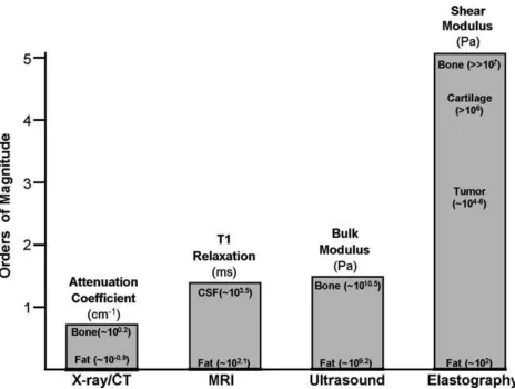
Figure 2: Imaging modality contrast mechanisms. Examples of different imaging modalities and the spectrum of contrast mechanisms utilized by them are shown. The shear modulus has the largest variation, with variations over five orders of magnitude among various physiological states of normal and pathologic tissues. (Reprinted with permission from Yogesh K. Mariappan, Kevin J. Glaser, Richard L. Ehman, “Magnetic resonance elastography: a review”, Clin Anat 23 no. 5 (2010): 497-511)

3.2 Manual Palpation

the subjective qualitative assessment of the physician; 3) MRE provides a 3D visualization of tissue biomechanics at high spatial resolution, as opposed to an average assessment for the bulk tissue volume; 4) for diseases like cancer, early detection greatly improves treatment outcome, and palpation cannot provide the same sensitivity as MRE to such early stage changes.

3.3 Alternative Elasticity Imaging Methods

MRE also has advantages over alternative elasticity imaging methods, such as optical coherence tomography elastography (van Soest et al. 2007), tissue Doppler optical coherence elastography (Wang, Ma, and Kirkpatrick 2006), ultrasound transient elastography (Sandrin et al. 2003), ultrasound shear wave elasticity imaging (Sarvazyan et al. 1998), and mechanical imaging (Sarvazyan 1998), in which stress patterns are measured on the tissue surface by a pressure sensor array.

MRE can provide measures from deep within the body, at high resolution and in a wide 3D field. Due to the absorption of light in biological tissue, optical based methods are limited to

superficial tissue. Likewise, ultrasound methods provide measures at limited depths due to the limited penetration of ultrasound in tissue, and only for a single direction and over a narrow field. Furthermore, MRE provides access to sites in the body that ultrasound cannot, e.g., the brain, for which the skull acts as an acoustic shield. Moreover, MRE can be applied for obese patients or when other factors may prevent ultrasound usage, such as ascites (fluid accumulation in the abdomen). Of course MRE is not feasible in patients with contraindications to MRI, such as those with pacemakers and cochlear implants, and might not tolerated by some patients, e.g., because of claustrophobia. Ultrasound elastography methods are not affected by these

4. Background of Magnetic Resonance Imaging

This section will provide a brief description of some of the basic principles behind MRI. For a fuller explanation readers are referred to MRI textbooks such as (McRobbie et al. 2007) and (Brown et al. 2014).

Magnetic resonance imaging is a diagnostic method based on the phenomenon of nuclear magnetic resonance. In the theory of quantum mechanics, elementary particles, composite particles (hadrons) and atomic nuclei carry a property of intrinsic angular momentum known as spin. Each kind of elementary particle has a particular magnitude of spin, which is indicated by an assigned spin quantum number, I, which can take only half integer or integer values. In MRI, Hydrogen (1H) is the element most commonly focused on, as it is the most abundant element in biological tissue (e.g., water and fat), although some work is carried out with other elements, including Sodium (23_{Na) and Phosphorus (}31_{P). The nucleus of the} 1_{H atom consists of one} proton, which is a composite particle with I=1/2. The intrinsic spin of the proton implies that it possesses angular momentum, p, which is related to I via:

𝐩= ℏ 𝐈 (1)

where ℏ = ℎ/2𝜋, h is Planck’s constant, and p and I are vector quantities. The proton also has a unit positive electric charge, and hence, in combination with its angular momentum, it is a “rotating charge”, with an associated magnetic dipole moment, :

𝛍 = 𝛾p (2)

2I+1 orientations with respect to the magnetic field, or 2I+1 energy levels. In the instance of the proton with I=1/2, the magnetic dipole moment can align with or against the magnetic field, which are the low and high energy states respectively (Figure 3). The energy difference between these two states, E, is proportional to the magnetic field strength, B0:

ΔE = μB₀⁄ = 𝛾ℏBI ₀ (3)

Figure 3: Energy level of diagram for the magnetic dipole moment of a proton

A transition can be induced between the energy states through applying electromagnetic radiation energy (radiowaves) of the appropriate frequency, L, called the Larmor frequency:

𝜔_𝐿 = Δ𝐸 ℏ = γB⁄ ₀ (4)

this mechanism the spatial location of the protons can be mapped through observing the frequency of the emitted radiation, and this is the underlying principle of MRI. The relative phase of neighboring proton spins can likewise be altered through application of a magnetic field gradient. The spins of protons that lie in different positions along the magnetic field gradient will rotate at different Larmor frequencies, and hence over time become out of phase with respect to each other. The electromagnetic radiation emitted by these protons will contain this phase information, and hence phase can be used in combination with frequency to locate the position of the emitting protons in two dimensions.

In the MRI scanner a magnetic field (B0) of typically 1.5 or 3 Tesla (T) field strength is applied, and various combinations of radiofrequency (RF) excitation pulses are delivered to the patient from radio-transmitter coils in the presence of magnetic field gradients, while the emitted radiation is detected by radio-receiver coils. The combinations of excitation pulses and gradients are commonly referred to as pulse sequences. A single implementation of the pulse sequence acquires one portion of the MRI data, and cycle is repeated at a fixed time interval (repetition time, denoted TR) until all the data is acquired.

the particular direction in space they are applied and the spatial encoding used.

The acquired RF signals are analyzed for frequency and phase, and the resulting data is stored as a spatial Fourier Transform, referred to as k-space, which at the end of data acquisition is converted into MR images through applying an inverse Fourier Transform. The MR images are signal maps, for which the signal strength at a given location is a function of the local concentration of protons (proton density) and other parameters associated with the chemical environment of the protons (the longitudinal relaxation time, T1) and the interaction of neighboring spins (the transverse relaxation time, T2). The signal contrast between different tissue types in MR images is caused by variations in these properties, and the pulse sequences are varied to emphasize different contrasts.

5. Magnetic Resonance Elastography Methodology

5.1 Dynamic MRE

5.1.1 Dynamic MRE Hardware

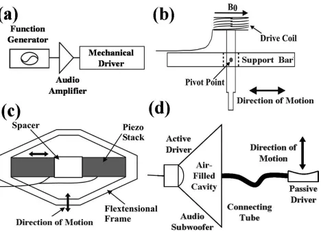
can be connected via an acoustic wave guide (air-filled tube) to an air-filled passive driver placed next to skin (Figure 5), which can take various shapes depending on the application (e.g., drum, disk or pillow). Alternatively a rigid rod or piston can be attached to the driver system which delivers vibrations via a rigid passive driver (Asbach et al. 2008, Sack, Beierbach, et al. 2009) (Figure 6). Longitudinal compression delivered at the skin is mode converted to shear waves at internal tissue boundaries. Pneumatic actuators can suffer from phase delays, which affect synchronization with the MRI sequence, particularly at higher frequencies. However they have the advantage of allowing high power amplification in the remote driver system, and are easily adaptable for wave delivery to the site of interest.

Electromechanical actuators consist of electromechanical voice coils, which when positioned in the main magnetic field of the MRI scanner, produce vibrations via the Lorentz force (Braun, Braun, and Sack 2003). Electromechanical actuators can achieve synchronization with the MRI sequence, and produce high amplitude waves. However, they also tend to provide limited power, can cause electromagnetic interference, and result in eddy currents in the RF receiver coils of the MRI scanner, which cause MRI artifacts and heating effects. As a result, electromechanical drivers must be positioned at a distance from the site of interest. They also have to be placed in a certain orientation with respect to the magnetic field of the MRI scanner.

Figure 4: External driver systems. (a): Block diagram of the external driver setup. Examples of typical mechanical drivers include (b) electromechanical, (c) piezoelectric-stack, and (d)

pressure-activated driver systems. (Reprinted with permission from Yogesh K. Mariappan, Kevin

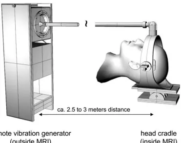
Figure 6: Head actuator used for stimulating low-frequency shear vibrations in the brain. The audio driver system is positioned outside the scan room, and is connected via a rigid piston to the head-cradle, which is fitted to the patient lying inside the MRI scanner. (Reprinted with

permission from Sack I, Beierbach B, Wuerfel J, Klatt D, Hamhaber U, Papazoglou S, Martus P, Braun J, “The impact of aging and gender on brain viscoelasticity”, Neuroimage 46 no.3 (2009): 652-657)

5.1.2 Dynamic MRE Pulse Sequences

be applied to capture motion in three orthogonal directions. The MSGs are applied in addition to the frequency- and phase-encoding and slice selective gradients used to map the positions of the emitting nuclei in the body.

The MRI scanner is triggered to coincide with the mechanical wave pulses. The spins of the hydrogen nuclei in the tissue are displaced in a cyclic motion by the mechanical waves, and when imaged in combination with the synchronized oscillating MSGs, the motion of the tissue is encoded as phase shifts in the MRI RF signal readout. At a given position vector (r) and relative phase of the MSG and mechanical waves (), the phase contribution () in the MR image due to the motion and MSG is:

𝜑(r,) =γ𝑁𝑇(G0⋅u0)

2 𝑐𝑜𝑠(𝐤 ⋅ 𝐫 +) (5)

where  is the gyromagnetic ratio, N the number of MSG gradient cycles, T the period of the MSG gradient waveform, G0 the MSG vector, u0 the displacement amplitude vector and the k

Figure 7: MRE pulse sequence diagram. RF= radiofrequency, GPhase= phase-encoding gradient, GRead= readout gradient or frequency-encoding gradient, Gslice = slice selective gradient. Motion sensitizing gradients (MSGs) are inserted in a spin echo sequence before and after the second RF impulse.  = phase offset between MSG and mechanical excitation. The MSG direction,

5.1.3 Dynamic MRE Inversion Methods

The inversion step calculates the mechanical properties from the measured displacement field, and produces a map of the properties, e.g., elasticity. Maps of the tissue elasticity are commonly termed “elastograms”. Numerous inversion methods have been developed (Doyley 2012), which employ various assumptions about factors such as the boundary conditions and tissue material properties. These methods have different strengths and weaknesses associated with inherent assumptions, or other factors such as the level of influence of imaging-related noise, which may be amplified through calculations. Generally inversion methods idealize biological tissue as a continuum and assume a particular material constitutive model, and many make the assumption, at least within regions, that the tissue is homogeneous, isotropic and linear viscoelastic. Hence, the greatest challenges for inversion methods occur in heterogeneous, anisotropic and complex material, when high spatial resolution is required, and the MRE data is affected by imaging-related noise.

5.1.3.1 Direct Inversion

Direct inversion is one of the more commonly used inversion methods for dynamic MRE. In harmonic MRE typically several acquisitions are made to measure the displacement field of the propagating mechanical wave at different snapshots in time. The measured data is processed by Fourier Transform to obtain the frequency domain complex displacement field, u, describing the steady-state:

u(𝐱, 𝑡) = u(𝐱)exp⁡(𝑖𝜔𝑡) (6)

Navier-Stokes equation for the propagation of an acoustic wave in a viscoelastic solid (Sinkus et al. 2005):

𝜕2_𝐮

𝜕2_𝑡⁡ = 𝜇𝛻

2 _{𝐮 + (+) .(∇ 𝐮) +}𝜕∇2𝐮

𝜕𝑡 +(+)

𝜕.(𝐮)

𝜕𝑡 (7)

where  is the material density,  the first Lamé parameter describing the material elasticity with regard to the compressional wave component,  the second Lamé parameter describing the material elasticity with respect to the shear wave component (note: this parameter is distinct from the magnetic dipole moment, ),  the viscosity of the compressional component, and  the shear viscosity. In a near incompressible medium such as biological tissue, the wavelength of the compressional component is typically very long (meters) while the amplitude is very small, and hence this component is very difficult to measure accurately. Furthermore, the compressional wave velocity tends to differ little between biological tissue types (typically 1540 m/s), while the shear wave velocity can differ substantially (1-10 m/s). Therefore, in dynamic MRE it is

typically the shear wave component of the displacement field that is focused on for measurement and characterization, and the task is to estimate  and . In near-incompressible material the gradient of the displacement field ∇𝐮 is very close to zero; perhaps indicating that one could neglect the second and fourth terms on the right hand side of Eq.7. However, while the very small compressional viscosity  might make it acceptable to ignore the fourth term, it is not safe to neglect the second term, as the large  of the near incompressible material balances the small .(∇ 𝐮). A preferred approach is to remove the contributions of the compressional wave

component from Eq.7, and one way to achieve this is by calculating the curl (divergence-free part) of the vector field (∇ × 𝐮 ) (Sinkus et al. 2005).

𝜕𝐯 𝜕𝑡 = 𝜇𝛻

2 _{𝐯 +}𝜕∇2𝐯

𝜕𝑡 (8)

Replacing 𝐮 with v in Eq.6 we get

𝐯(𝐱, 𝑡) = 𝐯(𝐱)exp⁡(𝑖𝜔𝑡) (9)

If this expression for 𝐯 is substituted into Eq.8 and the derivatives calculated we obtain a Helmholtz equation for the steady-state:

−𝜌𝜔2_{𝐯 = 𝜇∇}2_{𝐯 + 𝑖𝜔}_⁡∇2_{𝐯 (10)}

For 3D MRE data, by separating the components for the three dimensions, one obtains three equations for two unknowns,  and . By applying an assumption of local homogeneity of the material properties over the neighborhood of the voxel for derivative calculation, the equations can be solved separately for each voxel, using, for example, a least squares calculation (Sinkus et al. 2005). If the tissue is presumed to have near zero or negligible viscosity (0), Eq.10 is simplified to:

−𝜌𝜔2𝐯 = 𝜇∇2𝐯 (11)

This approach to inversion has also been described as algebraic inversion of the differential equation (AIDE) (Manduca et al. 2001). However, a full AIDE inversion described in (Oliphant et al. 2001) solves for both Lamé coeffients ( and ) for the compressional and shear wave components.

2D data, when using a high-pass filter, an assumption is made that the shear waves are

propagating parallel to the plane of the imaging slice, and if the direction of the wave is oblique to the slice this may lead to errors in the inversion estimates.

The variational inversion method described in (Romano, Shirron, and Bucaro 1998) avoids derivative calculations in solving for the Lamé coefficients ( and ) by using the weak or variational form of the Navier Stokes equation with appropriately chosen smooth test functions, and this approach allowed local inhomogeneity of the material parameters. (Honarvar et al. 2013) developed a curl-based finite element reconstruction based direct inversion method to solve for , that again used a weak formulation of the equation of motion, thereby allowing for local inhomogeneity of .

The shear wave parameters  and  are related to the complex shear modulus parameter 𝐺∗(𝜔), which relates complex stress 𝜎∗(𝜔) to complex strain 𝜖∗(𝜔).

𝜎∗_{(𝜔) = 𝐺}∗_(𝜔)𝜖∗_{(𝜔) = [𝐺}′_{(𝜔) + 𝑖𝐺}′′_(𝜔)]𝜖∗_{(𝜔) (12)}

where G' is the storage modulus and G'' the loss modulus, and 𝐺′_{(𝜔) = 𝜇 and 𝐺}′′_{(𝜔) = 𝜔}'. Hence, some MRE studies quote the viscoelastic measures in terms of G' and G'' (Sack, Beierbach, et al. 2009). Viscoelasticity can also be defined by the magnitude of the complex shear modulus (|𝐺∗_{|) in combination with the phase lag between stress and strain  (which is 0} for purely elastic material and 90° for purely viscous material), where 𝐺′ = |𝐺∗| cos 𝛿 and 𝐺′′ = |𝐺∗_{| sin 𝛿.}

measured wave speed to estimate shear stiffness. 5.1.3.2 Local Frequency Estimation

Another commonly used inversion approach for dynamic MRE is local frequency estimation (LFE). In this method the local spatial frequency, fsp, of the shear wave propagating pattern is measured. This can be estimated using an algorithm which combines measures over multiple scales obtained from wavelet filters (Manduca et al. 2001). The local spatial frequency is related to the local shear wave speed, cs, and the mechanical driving frequency fmech, i.e., cs= fmech/fsp. cs is also related to the complex shear modulus G*:

𝑐𝑠 = √

2|𝐺∗_|2

𝜌(𝑅𝑒(𝐺∗_)+|𝐺∗_|) (13)

where Re(G*) is the real component of G* (i.e., the storage modulus G’). For a material model with zero viscosity, this equation becomes:

𝜌𝑐_𝑠2 = 𝐺 (14)

where G is the shear modulus for which the imaginary component (the loss modulus, G'') is zero. The approximation of zero viscosity can be made for some tissues with low dispersion and attenuation. In this instance, G can be estimated from c2s as an effective “shear stiffness” (i.e., with the assumption of equal to that of water,1000 kg/m3). LFE is relatively robust to

imaging-related noise and can be implemented in 3D. However it makes the assumptions of local homogeneity, isotropy and incompressibility, has limited spatial resolution and is prone to

blurring at tissue boundaries. The phase gradient method (Catheline, Wu, and Fink 1999) is similar to the LFE method, however this time the local frequency is estimated from the gradient of the phase of the measured harmonic oscillation.

5.1.3.3 Other Dynamic MRE Inversion Methods

simulating the MRE displacement field with a set of material property parameters and comparing this with the acquired MRE data. For example, (Van Houten et al. 1999, VanHouten et al. 2003) have developed an iterative finite element model (FEM) based methodology to simulate the displacement fields, and to make the problem tractable for large data sets the data was separated into over-lapping subzones. Using this inversion method, parameters have also been calculated for a poroelastic material constitutive model, i.e., a solid elastic matrix permeated by fluid (Perrinez et al. 2010).

Other investigators have sought to characterize viscoelastic biological tissue according to its variable response to different mechanical frequencies, and have measured the complex shear modulus or wave speed at different frequencies. Multi-frequency measurements have been fit to candidate rheological models, such the Voigt and Spring-Pot models (Klatt et al. 2007, Sack, Beierbach, et al. 2009), and used to characterize of the exponent of a power law describing the behavior of the complex shear modulus (Sinkus et al. 2007). Multi-frequency measurements have also been summarized in combined multi-frequency parameters, such as multifrequency dual elastovisco inversion (MDEV) (Reiss-Zimmermann et al. 2014) and multi-frequency wave number recovery (Tzschatzsch et al. 2016). Post-processing algorithms for reducing the effects of imaging-related noise have also being explored (Barnhill et al. 2016).

5.2 Quasi-static MRE

5.2.1 Quasi-static MRE Hardware

For an in vivo breast study (Plewes et al. 2000) a quasi-static MRE device was constructed that attached to the breast RF coil of the MRI scanner, and breast tissue was compressed between two parallel plates, with one plate moving in and out in a sinusoidal motion, as driven by an

For an in vitro application (McGrath et al. 2012), a quasi-static MRE system was built for ex vivo prostate whole specimens, to determine the effect of exposure to pathology fixative

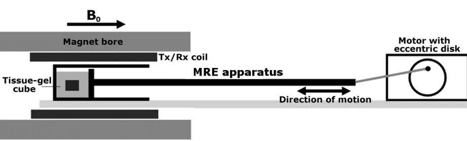
preserving solution (formaldehyde) on tissue elasticity. For this an apparatus was built in acrylic consisting of a holder and a compression plate, which was attached to a piston connected to an ultrasonic motor via an eccentric disk (Figure 8). The device was positioned in the bore of a 7-T preclinical MRI scanner, which was triggered by the motion of the piston. The tissue specimens were embedded in a block of gelatin before scanning, to provide stability during cyclic

compression.

Figure 8. Schematic of the quasi-static MRE device positioned within the scanner bore consisting of a sample holder (length = 20 cm, inside cross-sectional area = 8  8 cm2_{) in which the samples} are compressed by a square plate (8  8 cm2 _{surface area), which is attached via a mechanical} piston to the motor. (Reprinted with permission from Deirdre M. McGrath, Warren D. Foltz, Adil Al-Mayah, Carolyn J. Niu, Kristy K. Brock “Quasi-static magnetic resonance elastography at 7 T to measure the effect of pathology before and after fixation on tissue biomechanical properties”, Magn Reson Med. 68 no. 1 (2012):152-165)

5.2.2 Quasi-static MRE Pulse Sequences

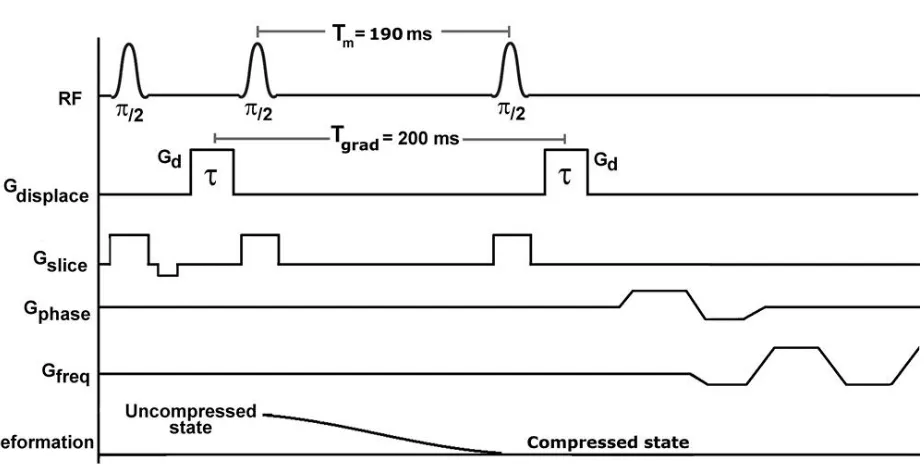
Chenevert et al. 1998, Plewes et al. 2000) (Figure 9). The STEAM pulse sequence includes three RF pulses, and for MRE two displacement encoding gradients are applied: one before the second RF pulse, and another after the third RF pulse. The displacement encoding gradients are

specified by the following parameters: gradient amplitude (Gd) and gradient duration (), which determine the displacement sensitivity (𝚽_𝑑 = 𝛾𝑮_𝑑𝜏), and the gradient pulse separation interval (Tgrad). The transition between the uncompressed and compressed states is timed to occur during the mixing time, Tm, between the second and third RF pulses. In (McGrath et al. 2012) echo planar imaging (EPI) was incorporated into the pulse sequence, to facilitate more rapid acquisition, as the application to pathology specimens was time sensitive, to limit tissue degradation before histopathology analysis. The pulse sequence was repeatedly applied to acquire the MRE data for the full imaging volume step by step, and the time to cycle through the pulse sequence (TR) was set to match the compression cycle time (1 s).

displacement-encoding gradients and EPI readout. The mechanical displacement from the uncompressed to compressed states occurs during the mixing time, Tm. Gdisplace = displacement encoding gradient. (Reprinted with permission from Deirdre M. McGrath, Warren D. Foltz, Adil Al-Mayah, Carolyn J. Niu, Kristy K. Brock “Quasi-static magnetic resonance elastography at 7 T to measure the effect of pathology before and after fixation on tissue biomechanical properties”,

Magn Reson Med. 68 no. 1 (2012):152-165)

5.2.3 Quasi-static MRE Inversion Methods

The displacement and strain patterns measured by elastography are related to the mechanical properties of the tissue, and for some applications visualization of the measured strain field in 2D or 3D may be sufficient to assess variations in elasticity, such as in the study by (Hardy et al. 2005) with ex vivo cartilage. However the strain field is also related to the deformational

geometry, and when more precise measurement of the elastic modulus is required a full inversion approach is adopted.

5.2.3.1 Direct Inversion

In the static or quasi-static case, the time derivative terms in the Navier-Stokes equation (Eq.7) are zero. For an incompressible material, the term 𝜆∇ ∙ 𝑢 is indeterminate, and in (Plewes et al. 2000, Bishop et al. 2000), this term was replaced by a parameter p, defined as average stress or pressure:

∇𝑝⁡ + 𝜇(∇2𝑢 + ∇∇ ∙ 𝑢) + (∇𝜇)(∇𝑢 + ∇𝑢Τ) = 0 (15)

boundary conditions for the unknown elastic modulus, and in (Plewes et al. 2000, Bishop et al. 2000) a constant boundary modulus was assumed for a relative modulus reconstruction, i.e., modulus values were constructed as ratios of the constant boundary value.This method assumes linear elasticity, small strain deformation and two-dimensional plane strain conditions, and these approximations make the matrix equation computationally tractable, with fewer unknown variables and spatial locations. (Chenevert et al. 1998) also carried out a direct inversion for quasi-static MRE, but applied another partial derivative to remove the pressure term. However, by including the pressure term as an unknown (Bishop et al. 2000, Plewes et al. 2000) avoided applying third order derivatives, which can be lead to amplification of imaging related noise. 5.2.3.2 Iterative Finite Element Model Based Inversion

Tissue deformation in static or quasi-static elastography can be deemed governable by equations of equilibrium and strain-displacement. The equilibrium equation of a continuum under static loading is therefore applicable:

3 , 2 , 1 0 3 3 2 2 1

1   

        i f x x x i i i

i  



(16)

where the s are the stress tensor components, fiare the body forces per unit volume, and X=

(x1,x2,x3) are Cartesian coordinates. For a linear elastic material under static deformation the strain (ij) tensor is:

              i j j i ij x u x u 2 1

 (17)





 _{ij ij kk}

ij E        2 1 1 (18)

where ij is the Kronecker delta symbol.

(Plewes et al. 2000) and (Samani, Bishop, and Plewes 2001) presented an iterative inversion method for quasi-static MRE which involved solving the so-called “forward problem”, by generating a simulated stress distribution from an estimated distribution of Young’s modulus. The forward solution was generated using a finite element model based simulation, which was a 3D contact problem with displacement boundary conditions specified by the plates of the

compression device. At each iteration E was updated according to an equation derived from Hooke’s law: i i i MRE i

E _{11 22 33}

11 1 1         (19)

where the updated modulus Ei+1of each finite element is calculated from one component of the MRE-measured strain (11MRE, the component parallel to the direction of motion of the

compression device) and the simulated three normal stress components of the previous iteration, combined with the assumed value for (for the assumption of near-incompressibility  was estimated at 0.499). The starting guess for E was estimated from the reciprocal of the measured strain. For the convergence metric the mean squared proportional differences between

consecutive modulus updates were compared with a defined tolerance, tol:

tol E E E i i i   1 (20)

the tissue into different types, e.g., for the breast: fat, fibroglandular tissue and tumor. At each iteration the new estimates for E were averaged across each tissue region. The final

reconstruction gave the relative average modulus values of the different inner regions with respect to the modulus of the outer region. Without knowledge of the true magnitude of the applied forces, the simulation produced a stress distribution with an arbitrary scaling, and hence the overall scaling of the estimated E values was also arbitrary. However, the relative distribution of modulus values will still be valid for the specified geometry and boundary conditions. As the algorithm only required a single component of strain (the normal component, 11 ), only a single motion encoding direction was needed in the direction of motion. Assuming a linear elastic material, 11 was calculable as u₁ x₁, which was calculated from the local MRI signal phase

and the displacement sensitivity, 𝚽𝑑.

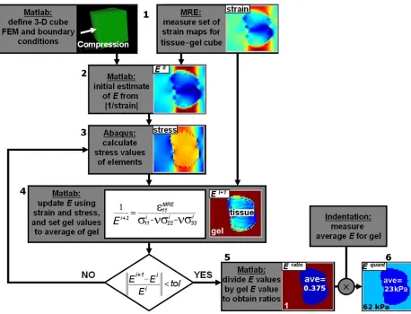
Figure 10. FEM iterative inversion algorithm for Quasi-static MRE (showing data from a simulation experiment): (1) finite elements and boundary conditions defined, and MRE used to measure strain; (2) strain used to estimate the initial E values; (3) ABAQUS (finite element solver) software simulates the compression and calculates three components of stress per

element; (4) MRE measured strain combined with calculated stress to provide new estimates of E and the gel E values are reset to their average, and convergence tested; (5) once converged, values are divided by the average gel value to obtain ratio-E values; and (6) multiplication by the indentation-measured gel E value to obtain quantitative E measures for tissue elements.

(Reprinted with permission from Deirdre M. McGrath, Warren D. Foltz, Adil Al-Mayah,

the effect of pathology before and after fixation on tissue biomechanical properties”, Magn Reson Med. 68 no. 1 (2012):152-165)

6. Applications of Magnetic Resonance Elastography

MRE has been applied to a wide range of organs and tissue types in humans and in animal models, both in vivo and in vitro. This section will provide an overview of MRE applications to date.

6.1 Clinical Applications

In vivo human MRE studies have been carried out for multiple organs and tissues including: liver (Venkatesh, Yin, and Ehman 2013, Rouviere et al. 2006, Huwart et al. 2007, Klatt et al. 2007, Huwart et al. 2006, Huwart et al. 2008, Godfrey et al. 2012, Singh et al. 2015, Su et al. 2014); spleen (Talwalkar et al. 2009); kidneys (Low, Owen, Joubert, Patterson, Graves, Glaser, et al. 2015, Rouviere et al. 2011, Lee et al. 2012); uterus and cervix (Jiang et al. 2014); pancreas (Venkatesh and Ehman 2015, Shi et al. 2015, Dittmann et al. 2016, An et al. 2016, Itoh et al. 2016); breast (McKnight et al. 2002, Plewes et al. 2000, Sinkus et al. 2000, Sinkus et al. 2005, VanHouten et al. 2003, Sinkus et al. 2007, Hawley et al. 2016); brain (Di Ieva et al. 2010, Guo et al. 2013, Braun et al. 2014, Sack et al. 2008, Murphy et al. 2011, Murphy et al. 2016, Romano et al. 2014, Sack, Beierbach, et al. 2009, Streitberger et al. 2014, Streitberger et al. 2012,

2014, Mariappan et al. 2011); head and neck (Yeung et al. 2013, Bahn et al. 2009). The following sections will expand on some of these clinical applications.

6.1.1 Liver

While most clinical MRE applications have been initial explorations of method feasibility and sensitivity to disease, liver MRE is a notable exception, as it has already been widely adopted in clinical practice for diagnosis of chronic liver disease (CLD), such as fibrosis (Figure 11). While biopsy is the gold standard diagnostic for liver fibrosis, it also carries the risks of an invasive procedure and is sometimes not tolerated by patients. Additionally, biopsy can be prone to error through sampling at the wrong locations, or if the sample volume is insufficient or of poor quality. MRE could be used instead of biopsy (Venkatesh, Yin, and Ehman 2013), for

longitudinal monitoring of disease progression or treatment, and also for guiding the selection of biopsy samples when histopathology is required (Perumpail et al. 2012). A number of studies have determined MRE to be a highly accurate diagnostic tool for CLD, with increases in liver stiffness accompanying progression through stages of fibrosis to cirrhosis (Singh et al. 2015, Su et al. 2014, Yin, Talwalkar, et al. 2007b). A recent comparison of MRE with diffusion weighted MRI for liver fibrosis, steatosis and inflammation demonstrated that MRE was more sensitive to the effects of fibrosis than the apparent diffusion coefficient (ADC), while MRE was less

al. 2008, Hennedige et al. 2016). Furthermore, a recent MRE study determined that liver biomechanics varied between children and adults (Etchell et al. 2016)

Figure 11. Early detection of fibrosis with MRE. Two patients with chronic hepatitis B. The patient in the upper row has normal liver stiffness, whereas the patient in the lower row has modestly elevated liver stiffness. Biopsies excluded fibrosis in the first patient and showed mild fibrosis in the second. All conventional MR images were normal in both patients. (Reprinted with permission from Sudhakar K. Venkatesh, Meng Yin, and Richard L. Ehman, “Magnetic resonance elastography of liver: technique, analysis, and clinical applications”, J Magn Reson Imaging 37 (2013): 544-555)

6.1.2 Spleen and Kidneys

In an MRE study by (Talwalkar et al. 2009) it was found that patients with CLD had a higher splenic stiffness compared with controls, and (Shin et al. 2014) found a positive linear

measurements before and after the placement of a transjugular intrahepatic portosystemic shunt. The number of renal MRE studies to date has been limited (Rouviere et al. 2011, Low, Owen, Joubert, Patterson, Graves, Glaser, et al. 2015), but the findings so far suggest a dependency of renal stiffness on liver fibrosis (Lee et al. 2012) and hepatorenal syndrome (HRS) (Low, Owen, Joubert, Patterson, Graves, Alexander, et al. 2015).

6.1.3 Brain

MRE has introduced the possibility of estimating in vivo brain tissue mechanics, as the skull acts as a barrier which precludes the use of other methods, such as palpation (except during surgery) and ultrasound based elastography. Initial investigations with brain MRE have found that cerebral biomechanical properties are dependent on age and gender (Arani et al. 2015, Sack, Beierbach, et al. 2009) and are sensitive to a variety of neurodegenerative and neurological diseases including Alzheimer’s disease (Murphy et al. 2011, Murphy et al. 2016) (Figures 12 and 13), Parkinson’s disease (Lipp et al. 2013), hydrocephalus pre- and post-shunt placement

(Streitberger et al. 2011, Freimann et al. 2012, Fattahi et al. 2016), and multiple sclerosis

(Wuerfel et al. 2010, Streitberger et al. 2012). Some initial MRE work with brain cancer patients has indicated that MRE may be used to distinguish different types of intracranial neoplasms, such as meningiomas and intra-axial neoplasms (Reiss-Zimmermann et al. 2014), and in (Sakai et al. 2016) meningiomas were found to be stiffer than pituitary adenomas.

However, the cerebral biomechanics measures for healthy volunteers have varied widely

between different studies, i.e., in a review (Di Ieva et al. 2010) found that for brain white matter

the shear modulus has varied between 2.5 and 15.2 kPa, and for grey matterbetween 2.8 and

12.9 kPa. Moreover the expected impact on cerebral biomechanics of neurodegenerative diseases

patients compared with healthy controls. While the different MRE measures for healthy brain might reflect heterogeneity across the population, recent studies have explored other potential influences, such as interference patterns from wave reflection and scattering at brain tissue boundaries. In (McGrath et al. 2015), using a FEM based brain MRE simulation, it was predicted that reflections from brain tissue interfaces with cranial features such as the falx cerebri could lead to inversion errors artifacts on the order of 10-20%, and that these errors would vary

an optimum methodology.

Figure 13. Example elastograms across the Alzeimer’s disease (AD) spectrum. Relative to a cognitively normal (CN) control subject, stiffness is elevated in low (but still positive) -amyloid subjects with MCI (la-MCI) before falling in high-amyloid subjects with MCI (ha-MCI) to levels that are common within the AD group. (MCI=mild cognitive impairment). (Reprinted with permission from Matthew C. Murphy, David T. Jones, Clifford R. Jack Jr., Kevin J. Glaser, Matthew L. Senjem, Armando Manduca, Joel P. Felmlee, Rickey E. Carter, Richard L. Ehman, John Huston III, “Regional brain stiffness changes across the Alzheimer's disease spectrum”,

NeuroImage: Clinical 10 (2016): 283–290)

6.1.4 Prostate

In vivo MRE methods for prostate are still in development, with different wave delivery methods being explored, i.e., via the rectum, perineum and pubic bone (Arani et al. 2013, Sahebjavaher et al. 2013, Li et al. 2011, Kemper et al. 2004, Sahebjavaher et al. 2014) (Figure 14). So far prostate MRE studies have demonstrated a potential utility to diagnose and locate prostate cancer, and distinguish cancer from benign prostatitis (Li et al. 2011). The accuracy of prostate cancer diagnosis with MRE has been evaluated through comparison of MRE of ex vivo whole

Figure 14. The images show the results of the transperineal motion-encoding gradient (MRE) approach in a patient prior to a radical prostatectomy procedure. The waves are present in all three directions in the entire gland, demonstrating the effectiveness of the transducer for inducing the waves, and the pulse sequence for encoding the resulting displacements. In the reconstructed elasticity image, the Gleason4 + 3 tumor can be identified (see matching histopathology slide). (Ax=axial imaging slice, Cor=coronal imaging slice). (Reprinted with permission from Ramin S. Sahebjavaher, Samuel Frew, Artem Bylinskii, Leon ter Beek, Philippe Garteiser, Mohammad Honarvar, Ralph Sinkus, and Septimiu Salcudean. Prostate MR elastography with transperineal electromagnetic actuation and a fast fractionally encoded steady-state gradient echo sequence.

NMR Biomed 27 no. 7 (2014):784-94)

6.1.5 Breast

Sinkus et al. 2007). Breast MRE has also been explored in combination with contrast enhanced MRI to improve breast cancer diagnosis (Siegmann et al. 2010).

6.1.6 Musculoskeletal

A wide range of musculoskeletal MRE studies have been carried out to measure muscle stiffness, and recent developments include implementation at high magnetic field strength (3 T) to

facilitate shorter patient scan times (Hong et al. 2016), and a pneumatic actuator which is adaptable to different shoulder shapes for examining supraspinatus muscle (Ito et al. 2016). The musculoskeletal MRE applications so far have included measurement for muscle cartography (Debernard et al. 2013) (Figure 15), muscle development from childhood to adulthood

Figure 15. A–I: MR and ultrasound elastographic images recorded in the same vastus medialis (VM) muscle of an adult in passive and active (10% and 20% of MVC) states. MVC= Maximum voluntary contraction. (Reprinted with permission from Laëtitia Debernard, Ludovic Robert, Fabrice Charleux, and Sabine F. Bensamoun.. A possible clinical tool to depict muscle elasticity mapping using magnetic resonance elastography. Muscle Nerve 47 no. 6 (2013):903-8.)

6.2 Pre-clinical Applications

vivo porcine lung (McGee, Hubmayr, and Ehman 2008). In another pulmonary application, proton (1_{H) MRE was carried out in ex vivo rat lung to explore measurement of normal and} edematous ventilator-injured lung (McGee et al. 2012).

For a cardiac MRE method, a model of myocardial hypertension with in vivo porcine heart was employed (Mazumder et al. 2016). MRE for the eye was explored using an ex vivo bovine globe model (Litwiller et al. 2010), and an applications for cartilage were tested using ex vivo bovine cartilage with dynamic MRE (Lopez et al. 2008), and quasi-static MRE (Hardy et al. 2005). In vivo mouse brain MRE methods were developed to measure demyelination in vivo in a murine model of multiple sclerosis (Schregel et al. 2012), and to measure the effects of stroke on brain viscoelastic properties (Freimann et al. 2013); and in both studies the MRE data were compared with histology. A microscopic MRE method was developed for ex vivo rat brain to study a traumatic brain injury model (Boulet, Kelso, and Othman 2011), and MRE was

employed to observe the development of post-natal rat brain in (Pong et al. 2016). Furthermore, MRE methodology was developed for in vivo ferret brain, incorporating a piezoelectric device which delivered waves via a bite-bar (Feng et al. 2013).

vivo after implantation in animal models (Othman et al. 2012). The potential of combining MRE with MR spectroscopy and other MRI parameters for tissue engineering is reviewed in (Kotecha, Klatt, and Magin 2013).

7 Future Challenges

A number of limitations and technical challenges remain before MRE can be adopted for the full gamut of prospective clinical applications. Patient scan times should be minimized as far as possible, but often full 3D coverage of an organ is required for accurate diagnosis, which implies a longer acquisition time. Innovations in MRE pulse sequences, such as the fractionally encoded gradient echo sequences in (Garteiser et al. 2013) and spatially selective excitations (Glaser, Felmlee, and Ehman 2006), will allow shorter scan times for full 3D coverage.

For dynamic MRE in viscoelastic tissue a trade-off exists between effective spatial resolution and coverage of the full tissue volume. The resolving power of MRE for features with varying elasticity is stronger at higher mechanical wave frequencies. However in viscoelastic media higher frequency waves are attenuated more rapidly, thereby limiting the distance from the driver for which adequate wave amplitudes may be measured. The issue of reduced coverage at higher frequencies might be offset by improved driver technology, such as the phased-array acoustic driver described in (Mariappan et al. 2009). Furthermore, stiffer tissues such as bone and cartilage require higher mechanical wave frequencies for dynamic MRE (on the order of kHz), and clinical MRI scanner hardware often does not allow delivery of oscillating motion encoding gradients at higher frequencies. Hence, hardware improvements are necessary for applications to high elastic modulus tissue, such as implemented for ex vivo bovine cartilage in (Lopez et al. 2008).

measured tissue biomechanics to the particular means of wave delivery, as predicted for brain MRE by the simulations in (McGrath et al. 2016). Hence, future studies should compare wave delivery methods for brain and other organ sites to determine the robustness and repeatability of measures, and to establish a consensus on the optimum wave delivery methods. Sensitivity to other methodological variations such as pulse sequences, imaging systems and magnetic field strengths must also be fully evaluated, such as in a recent study to determine the repeatability of liver stiffness measures (Trout et al. 2016). Another source of influence on MRE measures is the choice of inversion method employed, as some methods are prone to error, such as through amplification of imaging-related noise, or cannot handle the effects of wave interference. Further work is therefore required to determine the optimum inversion methods for different MRE applications, through comparison studies such as (Yoshimitsu et al. 2016). Moreover, as biological tissue often has heterogeneous and anisotropic material properties, development of inversion methods based on more complex material constitutive models is required, such as those already explored for anisotropic (Sinkus et al. 2000, Romano et al. 2012), heterogeneous

(Honarvar et al. 2013) and poroelastic material models of biological tissue (Perrinez et al. 2009).

8 Conclusions

applications before they can be fully adopted into routine clinical practice.

REFERENCES

An, H., Y. Shi, Q. Guo, and Y. Liu. 2016. Test-retest reliability of 3D EPI MR elastography of the pancreas. Clin Radiol 71 (10):1068 e7-1068 e12. doi: 10.1016/j.crad.2016.03.014. Anderson, A. T., E. E. Van Houten, M. D. McGarry, K. D. Paulsen, J. L. Holtrop, B. P. Sutton, J.

G. Georgiadis, and C. L. Johnson. 2016. Observation of direction-dependent mechanical properties in the human brain with multi-excitation MR elastography. J Mech Behav Biomed Mater 59:538-46. doi: 10.1016/j.jmbbm.2016.03.005.

Arani, A., M. Da Rosa, E. Ramsay, D. B. Plewes, M. A. Haider, and R. Chopra. 2013.

Incorporating endorectal MR elastography into multi-parametric MRI for prostate cancer imaging: Initial feasibility in volunteers. J Magn Reson Imaging 38 (5):1251-60. doi: 10.1002/jmri.24028.

Arani, A., K. L. Glaser, S. P. Arunachalam, P. J. Rossman, D. S. Lake, J. D. Trzasko, A. Manduca, K. P. McGee, R. L. Ehman, and P. A. Araoz. 2016. In vivo, high-frequency three-dimensional cardiac MR elastography: Feasibility in normal volunteers. Magn Reson Med. doi: 10.1002/mrm.26101.

Arani, A., M. C. Murphy, K. J. Glaser, A. Manduca, D. S. Lake, S. A. Kruse, C. R. Jack, Jr., R. L. Ehman, and J. Huston, 3rd. 2015. Measuring the effects of aging and sex on regional brain stiffness with MR elastography in healthy older adults. Neuroimage 111:59-64. doi: 10.1016/j.neuroimage.2015.02.016.

Med 60 (2):373-9. doi: 10.1002/mrm.21636.

Axel, L., and L. Dougherty. 1989. MR imaging of motion with spatial modulation of magnetization. Radiology 171 (3):841-5. doi: 10.1148/radiology.171.3.2717762. Bahn, M. M., M. D. Brennan, R. S. Bahn, D. S. Dean, J. L. Kugel, and R. L. Ehman. 2009.

Development and application of magnetic resonance elastography of the normal and pathological thyroid gland in vivo. J Magn Reson Imaging 30 (5):1151-4. doi: 10.1002/jmri.21963.

Barnhill, E., L. Hollis, I. Sack, J. Braun, P. R. Hoskins, P. Pankaj, C. Brown, E. J. van Beek, and N. Roberts. 2016. Nonlinear multiscale regularisation in MR elastography: Towards fine feature mapping. Med Image Anal 35:133-145. doi: 10.1016/j.media.2016.05.012. Basford, J. R., T. R. Jenkyn, K. N. An, R. L. Ehman, G. Heers, and K. R. Kaufman. 2002.

Evaluation of healthy and diseased muscle with magnetic resonance elastography. Arch Phys Med Rehabil 83 (11):1530-6.

Bensamoun, S. F., S. I. Ringleb, Q. Chen, R. L. Ehman, K. N. An, and M. Brennan. 2007. Thigh muscle stiffness assessed with magnetic resonance elastography in hyperthyroid patients before and after medical treatment. J Magn Reson Imaging 26 (3):708-13. doi:

10.1002/jmri.21073.

Bishop, J., A. Samani, J. Sciarretta, and D. B. Plewes. 2000. Two-dimensional MR elastography with linear inversion reconstruction: methodology and noise analysis. Phys Med Biol

45:2081-2091.

Boulet, T., M. L. Kelso, and S. F. Othman. 2011. Microscopic magnetic resonance elastography of traumatic brain injury model. J Neurosci Methods 201 (2):296-306. doi:

Brauck, K., C. J. Galban, S. Maderwald, B. L. Herrmann, and M. E. Ladd. 2007. Changes in calf muscle elasticity in hypogonadal males before and after testosterone substitution as monitored by magnetic resonance elastography. Eur J Endocrinol 156 (6):673-8. doi: 10.1530/eje-06-0694.

Braun, J., K. Braun, and I. Sack. 2003. Electromagnetic actuator for generating variably oriented shear waves in MR elastography. Magn Reson Med 50 (1):220-2. doi:

10.1002/mrm.10479.

Braun, J., J. Guo, R. Lutzkendorf, J. Stadler, S. Papazoglou, S. Hirsch, I. Sack, and J. Bernarding. 2014. High-resolution mechanical imaging of the human brain by three-dimensional multifrequency magnetic resonance elastography at 7T. Neuroimage

90:308-14. doi: 10.1016/j.neuroimage.2013.12.032.

Brown, Robert W, Y-C Norman Cheng, E Mark Haacke, Michael R Thompson, and Ramesh Venkatesan. 2014. Magnetic resonance imaging: physical principles and sequence design: John Wiley & Sons.

Catheline, S., F. Wu, and M. Fink. 1999. A solution to diffraction biases in sonoelasticity: the acoustic impulse technique. J Acoust Soc Am 105 (5):2941-50.

Chen, J., C. Ni, and T. Zhuang. 2005. Mechanical shear wave induced by piezoelectric ceramics for magnetic resonance elastography. Conf Proc IEEE Eng Med Biol Soc 7:7020-3. doi: 10.1109/iembs.2005.1616122.

reconstructive imaging by means of stimulated echo MRI. Magn Reson Med 39:482-490. Chopra, R., A. Arani, Y. Huang, M. Musquera, J. Wachsmuth, M. Bronskill, and D. Plewes.

2009. In vivo MR elastography of the prostate gland using a transurethral actuator. Magn Reson Med 62:665-671.

Curtis, E. T., S. Zhang, V. Khalilzad-Sharghi, T. Boulet, and S. F. Othman. 2012. Magnetic resonance elastography methodology for the evaluation of tissue engineered construct growth. J Vis Exp (60). doi: 10.3791/3618.

Damughatla, A. R., B. Raterman, T. Sharkey-Toppen, N. Jin, O. P. Simonetti, R. D. White, and A. Kolipaka. 2015. Quantification of aortic stiffness using MR elastography and its comparison to MRI-based pulse wave velocity. J Magn Reson Imaging 41 (1):44-51. doi: 10.1002/jmri.24506.

Debernard, L., L. Robert, F. Charleux, and S. F. Bensamoun. 2011. Analysis of thigh muscle stiffness from childhood to adulthood using magnetic resonance elastography (MRE) technique. Clin Biomech (Bristol, Avon) 26 (8):836-40. doi:

10.1016/j.clinbiomech.2011.04.004.

Debernard, L., L. Robert, F. Charleux, and S. F. Bensamoun. 2013. A possible clinical tool to depict muscle elasticity mapping using magnetic resonance elastography. Muscle Nerve

47 (6):903-8. doi: 10.1002/mus.23678.

Di Ieva, A., F. Grizzi, E. Rognone, Z. T. Tse, T. Parittotokkaporn, Y. Baena F. Rodriguez, M. Tschabitscher, C. Matula, S. Trattnig, and Y. Baena R. Rodriguez. 2010. Magnetic resonance elastography: a general overview of its current and future applications in brain imaging. Neurosurg Rev 33 (2):137-45; . doi: 10.1007/s10143-010-0249-6.

Tomoelastography of the abdomen: Tissue mechanical properties of the liver, spleen, kidney, and pancreas from single MR elastography scans at different hydration states.

Magn Reson Med. doi: 10.1002/mrm.26484.

Domire, Z. J., M. B. McCullough, Q. Chen, and K. N. An. 2009. Feasibility of using magnetic resonance elastography to study the effect of aging on shear modulus of skeletal muscle.

J Appl Biomech 25 (1):93-7.

Doyley, M. M. 2012. Model-based elastography: a survey of approaches to the inverse elasticity problem. Phys Med Biol 57 (3):R35-73. doi: 10.1088/0031-9155/57/3/r35.

Ehman, E. C., P. J. Rossman, S. A. Kruse, A. V. Sahakian, and K. J. Glaser. 2008. Vibration safety limits for magnetic resonance elastography. Phys Med Biol 53 (4):925-35. doi: 10.1088/0031-9155/53/4/007.

Elgeti, T., M. Laule, N. Kaufels, J. Schnorr, B. Hamm, A. Samani, J. Braun, and I. Sack. 2009. Cardiac MR elastography: comparison with left ventricular pressure measurement. J Cardiovasc Magn Reson 11:44. doi: 10.1186/1532-429x-11-44.

Etchell, E., L. Juge, A. Hatt, R. Sinkus, and L. E. Bilston. 2016. Liver Stiffness Values Are Lower in Pediatric Subjects Than in Adults and Increase with Age: A Multifrequency MR Elastography Study. Radiology:160252. doi: 10.1148/radiol.2016160252.

Fattahi, N., A. Arani, A. Perry, F. Meyer, A. Manduca, K. Glaser, M. L. Senjem, R. L. Ehman, and J. Huston. 2016. MR Elastography Demonstrates Increased Brain Stiffness in Normal Pressure Hydrocephalus. AJNR Am J Neuroradiol 37 (3):462-7. doi:

10.3174/ajnr.A4560.

excitation of intracranial shear waves. NMR Biomed 28:1426-1432.

Feng, Y., E. H. Clayton, Y. Chang, R. J. Okamoto, and P. V. Bayly. 2013. Viscoelastic properties of the ferret brain measured in vivo at multiple frequencies by magnetic resonance elastography. J Biomech 46 (5):863-70. doi: 10.1016/j.jbiomech.2012.12.024. Freimann, F. B., S. Muller, K. J. Streitberger, J. Guo, S. Rot, A. Ghori, P. Vajkoczy, R. Reiter, I. Sack, and J. Braun. 2013. MR elastography in a murine stroke model reveals correlation of macroscopic viscoelastic properties of the brain with neuronal density. NMR Biomed

26 (11):1534-9. doi: 10.1002/nbm.2987.

Freimann, F. B., K. J. Streitberger, D. Klatt, K. Lin, J. McLaughlin, J. Braun, C. Sprung, and I. Sack. 2012. Alteration of brain viscoelasticity after shunt treatment in normal pressure hydrocephalus. Neuroradiology 54 (3):189-96. doi: 10.1007/s00234-011-0871-1. Gallichan, D., M. D. Robson, A. Bartsch, and K. L. Miller. 2009. TREMR: Table-resonance

elastography with MR. Magn Reson Med 62 (3):815-21. doi: 10.1002/mrm.22046. Garteiser, P., R. S. Sahebjavaher, L. C. Ter Beek, S. Salcudean, V. Vilgrain, B. E. Van Beers,

and R. Sinkus. 2013. Rapid acquisition of multifrequency, multislice and multidirectional MR elastography data with a fractionally encoded gradient echo sequence. NMR Biomed

26 (10):1326-35. doi: 10.1002/nbm.2958.

Glaser, K. J., J. P. Felmlee, and R. L. Ehman. 2006. Rapid MR elastography using selective excitations. Magn Reson Med 55 (6):1381-9. doi: 10.1002/mrm.20913.

10.1007/s00330-012-2527-x.

Goss, S. A., R. L. Johnston, and F. Dunn. 1978. Comprehensive compilation of empirical ultrasonic properties of mammalian tissues. J Acoust Soc Am 64 (2):423-57.

Green, M. A., L. E. Bilston, and R. Sinkus. 2008. In vivo brain viscoelastic properties measured by magnetic resonance elastography. NMR Biomed 21 (7):755-64. doi:

10.1002/nbm.1254.

Guo, J., C. Buning, E. Schott, T. Kroncke, J. Braun, I. Sack, and C. Althoff. 2015. In vivo abdominal magnetic resonance elastography for the assessment of portal hypertension before and after transjugular intrahepatic portosystemic shunt implantation. Invest Radiol

50 (5):347-51. doi: 10.1097/rli.0000000000000136.

Guo, J., S. Hirsch, A. Fehlner, S. Papazoglou, M. Scheel, J. Braun, and I. Sack. 2013. Towards an elastographic atlas of brain anatomy. PLOS ONE 8 (8):e71807. doi:

10.1371/journal.pone.0071807.

Hardy, P. A., A. C. Ridler, C. B. Chiarot, D. B. Plewes, and R. M. Henkelman. 2005. Imaging articular cartilage under compression--cartilage elastography. Magn Reson Med 53 (5):1065-73. doi: 10.1002/mrm.20439.

Hawley, J. R., P. Kalra, X. Mo, B. Raterman, L. D. Yee, and A. Kolipaka. 2016. Quantification of breast stiffness using MR elastography at 3 Tesla with a soft sternal driver: A

reproducibility study. J Magn Reson Imaging. doi: 10.1002/jmri.25511.

Heers, G., T. Jenkyn, M. A. Dresner, M. O. Klein, J. R. Basford, K. R. Kaufman, R. L. Ehman, and K. N. An. 2003. Measurement of muscle activity with magnetic resonance

elastography. Clin Biomech (Bristol, Avon) 18 (6):537-42.

Madhavan, A. Wee, and S. K. Venkatesh. 2016. Comparison of magnetic resonance elastography and diffusion-weighted imaging for differentiating benign and malignant liver lesions. Eur Radiol 26 (2):398-406. doi: 10.1007/s00330-015-3835-8.

Hirsch, S., D. Klatt, F. Freimann, M. Scheel, J. Braun, and I. Sack. 2013. In vivo measurement of volumetric strain in the human brain induced by arterial pulsation and harmonic waves.

Magn Reson Med 70 (3):671-83. doi: 10.1002/mrm.24499.

Honarvar, M., R. Sahebjavaher, R. Sinkus, R. Rohling, and S. Salcudean. 2013. Curl-based Finite Element Reconstruction of the Shear Modulus Without Assuming Local Homogeneity: Time Harmonic Case. IEEE Trans Med Imaging. doi:

10.1109/tmi.2013.2276060.

Hong, S. H., S. J. Hong, J. S. Yoon, C. H. Oh, J. G. Cha, H. K. Kim, and B. Bolster, Jr. 2016. Magnetic resonance elastography (MRE) for measurement of muscle stiffness of the shoulder: feasibility with a 3 T MRI system. Acta Radiol 57 (9):1099-106. doi: 10.1177/0284185115571987.

Huwart, L., F. Peeters, R. Sinkus, L. Annet, N. Salameh, L. C. ter Beek, Y. Horsmans, and B. E. Van Beers. 2006. Liver fibrosis: non-invasive assessment with MR elastography. NMR Biomed 19:173-179.

Huwart, L., C. Sempoux, N. Salameh, J. Jamart, L. Annet, R. Sinkus, F. Peeters, L. C. ter Beek, Y. Horsmans, and B. E. Van Beers. 2007. Liver fibrosis: noninvasive assessment with MR elastography versus aspartate aminotransferase-to-platelet ratio index. Radiology

245 (2):458-466.

elastography for the noninvasive staging of liver fibrosis. Gastroenterology 135 (1):32-40. doi: 10.1053/j.gastro.2008.03.076.

Ito, D., T. Numano, K. Mizuhara, K. Takamoto, T. Onishi, and H. Nishijo. 2016. A new

technique for MR elastography of the supraspinatus muscle: A gradient-echo type multi-echo sequence. Magn Reson Imaging 34 (8):1181-8. doi: 10.1016/j.mri.2016.06.003. Itoh, Y., Y. Takehara, T. Kawase, K. Terashima, Y. Ohkawa, Y. Hirose, A. Koda, N. Hyodo, T.

Ushio, Y. Hirai, N. Yoshizawa, S. Yamashita, H. Nasu, N. Ohishi, and H. Sakahara. 2016. Feasibility of magnetic resonance elastography for the pancreas at 3T. J Magn Reson Imaging 43 (2):384-90. doi: 10.1002/jmri.24995.

Jenkyn, T. R., R. L. Ehman, and K. N. An. 2003. Noninvasive muscle tension measurement using the novel technique of magnetic resonance elastography (MRE). J Biomech 36 (12):1917-21.

Jiang, X., P. Asbach, K. J. Streitberger, A. Thomas, B. Hamm, J. Braun, I. Sack, and J. Guo. 2014. In vivo high-resolution magnetic resonance elastography of the uterine corpus and cervix. Eur Radiol 24 (12):3025-33. doi: 10.1007/s00330-014-3305-8.

Kemper, J., R. Sinkus, J. Lorenzen, C. Nolte-Ernsting, A. Stork, and G. Adam. 2004. MR elastography of the prostate: Initial in-vivo application. Rofo. Fortschritte auf dem Gebiet der Rontgenstrahlen und der bildgebenden Verfahren 176 (8):1094-1099.

Kenyhercz, W. E., B. Raterman, V. S. Illapani, J. Dowell, X. Mo, R. D. White, and A. Kolipaka. 2016. Quantification of aortic stiffness using magnetic resonance elastography:

Measurement reproducibility, pulse wave velocity comparison, changes over cardiac cycle, and relationship with age. Magn Reson Med 75 (5):1920-6. doi:

Klatt, D., U. Hamhaber, P. Asbach, J. Braun, and I. Sack. 2007. Noninvasive assessment of the rheological behavior of human organs using multifrequency MR elastography: a study of brain and liver viscoelasticity. Phys Med Biol 52:7281-7294.

Kolipaka, A., V. S. Illapani, P. Kalra, J. Garcia, X. Mo, M. Markl, and R. D. White. 2016. Quantification and comparison of 4D-flow MRI-derived wall shear stress and MRE-derived wall stiffness of the abdominal aorta. J Magn Reson Imaging. doi:

10.1002/jmri.25445.

Kolipaka, A., D. Woodrum, P. A. Araoz, and R. L. Ehman. 2012. MR elastography of the in vivo abdominal aorta: a feasibility study for comparing aortic stiffness between hypertensives and normotensives. J Magn Reson Imaging 35 (3):582-6. doi: 10.1002/jmri.22866. Kotecha, M., D. Klatt, and R. L. Magin. 2013. Monitoring cartilage tissue engineering using

magnetic resonance spectroscopy, imaging, and elastography. Tissue Eng Part B Rev 19 (6):470-84. doi: 10.1089/ten.TEB.2012.0755.

Lee, C. U., J. F. Glockner, K. J. Glaser, M. Yin, J. Chen, A. Kawashima, B. Kim, W. K. Kremers, R. L. Ehman, and J. M. Gloor. 2012. MR elastography in renal transplant patients and correlation with renal allograft biopsy: a feasibility study. Acad Radiol 19 (7):834-41. doi: 10.1016/j.acra.2012.03.003.

Leitao, H. S., S. Doblas, P. Garteiser, G. d'Assignies, V. Paradis, F. Mouri, C. F. Geraldes, M. Ronot, and B. E. Van Beers. 2016. Hepatic Fibrosis, Inflammation, and Steatosis: Influence on the MR Viscoelastic and Diffusion Parameters in Patients with Chronic Liver Disease. Radiology:151570. doi: 10.1148/radiol.2016151570.

doi: 10.1258/ar.2010.100276.

Lipp, A., R. Trbojevic, F. Paul, A. Fehlner, S. Hirsch, M. Scheel, C. Noack, J. Braun, and I. Sack. 2013. Cerebral magnetic resonance elastography in supranuclear palsy and idiopathic Parkinson's disease. Neuroimage Clin 3:381-7. doi:

10.1016/j.nicl.2013.09.006.

Litwiller, D.V., S.J. Lee, A. Kolipaka, Y.K. Mariappan, K. J. Glaser, J.S. Pulido, and R. L. Ehman. 2010. Magnetic resonance elastography of the ex-vivo bovine globe. J Magn Reson Imaging 32 (1):44-51.

Lopez, O., K. K. Amrami, A. Manduca, and R. L. Ehman. 2008. Characterization of the dynamic shear properties of hyaline cartilage using high frequency dynamic MR elastography.

Magn Reson Med 59:356-364.

Lorenzen, J., R. Sinkus, M. Lorenzen, M. Dargatz, C. Leussler, P. Roschmann, and G. Adam. 2002. MR elastography of the breast:preliminary clinical results. Rofo 174 (7):830-4. doi: 10.1055/s-2002-32690.

Low, G., N. E. Owen, I. Joubert, A. J. Patterson, M. J. Graves, G. J. Alexander, and D. J. Lomas. 2015. Magnetic resonance elastography in the detection of hepatorenal syndrome in patients with cirrhosis and ascites. Eur Radiol 25 (10):2851-8. doi: 10.1007/s00330-015-3723-2.

Manduca, A., T. E. Oliphant, M. A. Dresner, J. L. Mahowald, S. A. Kruse, E. Amromin, J. P. Felmlee, J. F. Greenleaf, and R. L. Ehman. 2001. Magnetic resonance elastography: non-invasive mapping of tissue elasticity. Med Image Anal 5:237-254.

Mariappan, Y. K., K. J. Glaser, R. D. Hubmayr, A. Manduca, R. L. Ehman, and K. P. McGee. 2011. MR elastography of human lung parenchyma: technical development, theoretical modeling and in vivo validation. J Magn Reson Imaging 33 (6):1351-61. doi:

10.1002/jmri.22550.

Mariappan, Y. K., K. J. Glaser, D. L. Levin, R. Vassallo, R. D. Hubmayr, C. Mottram, R. L. Ehman, and K. P. McGee. 2014. Estimation of the absolute shear stiffness of human lung parenchyma using (1) H spin echo, echo planar MR elastography. J Magn Reson

Imaging 40 (5):1230-7. doi: 10.1002/jmri.24479.

Mariappan, Y. K., P. J. Rossman, K. J. Glaser, A. Manduca, and R. L. Ehman. 2009. Magnetic resonance elastography with a phased-array acoustic driver system. Magn Reson Med 61 (3):678-85. doi: 10.1002/mrm.21885.

Mariappan, Y.K., K. J. Glaser, and R. L. Ehman. 2010. Magnetic resonance elastography: a review. Clin Anat 23:497-511.

Mazumder, R., S. Schroeder, X. Mo, B. D. Clymer, R. D. White, and A. Kolipaka. 2016. In vivo quantification of myocardial stiffness in hypertensive porcine hearts using MR

elastography. J Magn Reson Imaging. doi: 10.1002/jmri.25423.

McCracken, P. J., A. Manduca, J. Felmlee, and R. L. Ehman. 2005. Mechanical transient-based magnetic resonance elastography. Magn Reson Med 53 (3):628-39. doi:

10.1002/mrm.20388.

2011. Evaluation of muscles affected by myositis using magnetic resonance elastography.

Muscle Nerve 43 (4):585-90. doi: 10.1002/mus.21923.

McGee, K. P., R. D. Hubmayr, and R. L. Ehman. 2008. MR elastography of the lung with hyperpolarized 3He. Magn Reson Med 59:14-18.

McGee, K. P., Y. K. Mariappan, R. D. Hubmayr, R. E. Carter, Z. Bao, D. L. Levin, A. Manduca, and R. L. Ehman. 2012. Magnetic resonance assessment of parenchymal elasticity in normal and edematous, ventilator-injured lung. J Appl Physiol 113 (4):666-76. doi: 10.1152/japplphysiol.01628.2011.

McGrath, D. M., W. D. Foltz, A. Al-Mayah, C. J. Niu, and K. K. Brock. 2012. Quasi-static magnetic resonance elastography at 7 T to measure the effect of pathology before and after fixation on tissue biomechanical properties. Magn Reson Med 68 (1):152-65. doi: 10.1002/mrm.23223.

McGrath, D. M., N. Ravikumar, L. Beltrachini, I. D. Wilkinson, A. F. Frangi, and Z. A. Taylor. 2016. Evaluation of wave delivery methodology for brain MRE: Insights from

computational simulations. Magn Reson Med. doi: 10.1002/mrm.26333.

McGrath, D.M., W.D. Foltz, N. Samavati, J. Lee, M.A. Jewett, T.H. van der Kwast, C. Menard, and K.K. Brock. 2011. Biomechanical property quantification of prostate cancer by quasi-static MR elastography at 7 tesla of radical prostatectomy, and correlation with whole mount histology. Proc Intl Soc Mag Res Med 19:1483.

McKnight, A. L., J. L. Kuge, P. J. Rossman, A. Manduca, L. C. Hartman, and R. L. Ehman. 2002. MR elastography of breast cancer: preliminary results. Amer J Roent 178:1411-1417.