ROSEFW-RF: The winner algorithm for the ECBDL’14
Big Data Competition: An extremely imbalanced big
data bioinformatics problem
Isaac Trigueroa,b,, Sara del R´ıoc, Victoria L´opezc, Jaume Bacarditd, Jos´e M.
Ben´ıtezc, Francisco Herrerac
a
Department of Respiratory Medicine, Ghent University, 9000 Gent, Belgium b
VIB Inflammation Research Center, 9052 Zwijnaarde, Belgium c
Department of Computer Science and Artificial Intelligence, CITIC-UGR (Research Center on Information and Communications Technology). University of
Granada, 18071 Granada, Spain d
Interdisciplinary Computing and Complex BioSystems (ICOS) Research Group, School of Computing Science, Newcastle University, Newcastle upon Tyne, NE1 7RU, United
Kingdom
Abstract
The application of data mining and machine learning techniques to bio-logical and biomedicine data continues to be an ubiquitous research theme in current bioinformatics. The rapid advances in biotechnology are allowing us to obtain and store large quantities of data about cells, proteins, genes, etc, that should be processed. Moreover, in many of these problems such as contact map prediction, the problem tackled in this paper, it is difficult to collect representative positive examples. Learning under these circumstances, known as imbalanced big data classification, may not be straightforward for most of the standard machine learning methods.
In this work we describe the methodology that won the ECBDL’14 big data challenge for a bioinformatics big data problem. This algorithm, named as ROSEFW-RF, is based on several MapReduce approaches to (1) balance the classes distribution through random oversampling, (2) detect the most relevant features via an evolutionary feature weighting process and a
old to choose them, (3) build an appropriate Random Forest model from the pre-processed data and finally (4) classify the test data. Across the paper, we detail and analyze the decisions made during the competition showing an extensive experimental study that characterize the way of working of our methodology. From this analysis we can conclude that this approach is very suitable to tackle large-scale bioinformatics classifications problems.
Keywords:
Bioinformatics, Big data, Hadoop, MapReduce, Imbalance classification, Evolutionary feature selection
1. Introduction
Data mining and machine learning techniques [1] have become a need in many Bioinformatics applications [2, 3, 4]. The application of these methods has shown to be very helpful for the extraction of useful information from data in a wide variety of biological problems such as genomics, proteomics, microarrays, etc [5]. The complexity and gigantic amount of biological data relate to several major issues that data mining tools have to address:
• High dimensional nature: Most biological problems, going from sequence analysis over microarray analysis to spectral analyses, natu-rally present a great number of characteristics. Hence, the application of data mining methods to such kind of data is generally affected by the curse of dimensionality. For this reason, the use of preprocess-ing techniques has been widely extended in bioinformatics. Two main alternatives have been applied in the literature: dimensionality reduc-tion [6] or feature selecreduc-tion [7]. The former is based on projecreduc-tion (for instance, principal component analysis) or compression (by using in-formation theory). The latter aims at preserving the original semantics of the variable by choosing a subset of the original set of features.
[11], which transform somehow the original training set, and algorith-mic modifications which modify current algorithm implementations in order to benefit the classification of the minority class.
• Large-scale: The unstoppable advance of the technologies has im-proved the collection process of new biological data. Dealing with very large amounts of data efficiently is not straightforward for machine learning methods. The interest of developing really scalable machine learning models for big data problems are growing up in the recent years by proposing distributed-based models [12, 13]. Examples of parallel classification techniques are [14, 15, 16]. They have shown that the distribution of the data and the processing under a cloud computing infrastructure is very useful for speeding up the knowledge extraction process.
When the first two issues are raised together with a high number of ex-amples, current approaches become non effective and non efficient due to the big dimension of the problem. Therefore, the design of new algorithms will be necessary to overtake the mentioned limitations in the big data framework (see the three recent reviews focusing the big data analytics an technologies [12, 17, 18]).
Ensemble-based classifiers are a popular choice in the area of bioinformat-ics due to their unique advantages in dealing with high-dimensionality and complex data structures and their flexibility to be adapted to different kind of problems. New developments are continuously being published for a wide variety of classification purposes [19, 20]. Among the different ensemble-based techniques, the Random Forest (RF) algorithm [21] is a well-known decision tree ensemble method that has highlighted in bioinformatics [22] because of its robustness and good performance. Some efforts to accelerate the execution of this method for large scale problems have been very recently proposed [23, 24].
considered in this competition was formed by 32 million instances, 631 at-tributes, 2 classes, 98% of negative examples. Thus, it will require methods that can cope with high-dimensional imbalanced big data problems.
In this work we describe step-by-step the methodology with which we have participated, under the name ’Efdamis’, in the ECBDL’14 competition, ranking as the winner algorithm. We focused on MapReduce [29] paradigm in order to manage this voluminous data set. Thus, we extended the applicabil-ity of some pre-processing and classification models to deal with large-scale problems. We will detail the decisions made during the competition that leaded us to develop the final method we present here. This is composed of four main parts:
1. An oversampling approach: The goal of this phase is to balance the highly imbalanced class distribution of the given problem by replicating randomly the instances of the minority class. To do so, we follow a data-level approach presented in our previous work [23] for imbalanced big data classification.
2. An evolutionary feature weighting method: Due the relative high number of features of the given problem we needed to develop a feature selection scheme for large-scale problems that improves the classifica-tion performance by detecting the most significant features. To do this, we were based on a differential evolution feature weighting scheme pro-posed in [30] coupled with a threshold parameter to choose the most confident ones.
3. Building a learning model: As classifier, we focused on the RF algorithm. Concretely, we utilized the Random Forest implementation of Mahout [31] for big data.
4. Testing the model: Even the test data can be considered big data (2.9 millions of instances), so that, it was necessary to deploy the test-ing phase within a parallel approach that allow us to obtain a rapid response of our algorithm.
The rest of the paper is organized as follows. In Section 2, we provide background information about the problem of contact map prediction. Sec-tion 3 describes the MapReduce framework for big data. In SecSec-tion 4, we will describe step by step the design decisions we took during the compe-tition, arising into the final algorithm. Finally, Section 5 summarizes the conclusions of the paper.
2. Contact map prediction
Contact Map (CM) prediction is a bioinformatics (and specifically a pro-tein structure prediction) classification task that is an ideal test case for a big data challenge for several reasons. As the next paragraphs will detail, CM data sets easily reach tens of millions of instances, hundreds (if not thou-sands) of attributes and have an extremely high class imbalance. In this section we describe in detail the steps for the creation of the data set used to train the CM prediction method of [26].
2.1. Protein Structure Prediction and Contact Map
to estimate, using classification techniques, the whole CM matrix from the amino acid composition of a protein sequence.
2.2. Selection of proteins for the data set
In order to generate the training set for the CM prediction method we need proteins with known structure. These are taken from the Protein Data Bank (PDB) public repository that currently holds the structures of 80K proteins. A subset of 2682 proteins from PDB was selected with the follow-ing criteria: (1) Selectfollow-ing structures that were experimentally known with good resolution (less than 2˚A), (2) that no proteins in the set had a pair-wise amino-acid composition similarity of +30% and (3) that no protein had breaks in the sequence or non-standard amino acids. From all proteins matching three criteria we kept all proteins with less than 250 amino acids and a randomly selected 20% of proteins of larger size (in order to limit the number of pairs of amino acids in the data set). The set of proteins was split 90%-10% into training and test sets. The training set had 32M pairs of amino acids and the test set had 2.9M.
2.3. Representation
The representation used to characterise pairs of amino acids for CM pre-diction is composed of 631 attributes, split in three main parts that are represented in Figure 1:
Figure 1: Representation of the contact map prediction data set. 1: Detail information of selected positions in the protein sequence. 2: Statistics of the segment connecting the target pair of amino acids. 3: Global protein information
2. Statistics about the sequence segment connecting the target pair of amino acids. The whole segment between the two amino acids to be tested for contact is characterised as the frequency of the 20 amino acids types in the segment, frequency of the three secondary structure states, five contact number states, five solvent accessibility states and five recursive convex hull states: 38 attributes in total.
3. Global protein sequence information. The overall sequence is also char-acterised exactly in the same way as the connecting segment above (38 attributes) plus three extra individual attributes: the length of the protein sequence, the number of amino acids apart that the target pair are and finally a statistical contact propensity between the amino acid types of the pair of amino acids to be tested for contact. 41 attributes in total.
2.4. Scoring of predictions for the ECBDL’14 big data challenge
In the ECBDL’14 big data challenge three metrics were used to asses the prediction results: true positive rate (TPR: TP/P), true negative rate (TNR: TN/N), accuracy, and the final score of TPR· TNR1. The final score
was chosen because of the huge class imbalance of the data set in order to reward methods that try to predict well the minority class of the problem. These evaluation criteria are quite different from the standard criteria used by the PSP community to evaluate CM prediction methods [35], in which predictors are asked to submit a confidence interval [0,1] for each predicted
contact, and performance is evaluated separately for each protein by sort-ing predictions by confident and then selectsort-ing a subset of predictions for each protein proportional to the protein’s size. The precision of the predic-tor (TP/(TP+FP)) for a protein is computed from this subset of predicted contacts. Hence, the results of the ECBDL’14 competition are not directly comparable to standard CM prediction methods, but nonetheless it is still a very challenging big data task.
3. MapReduce
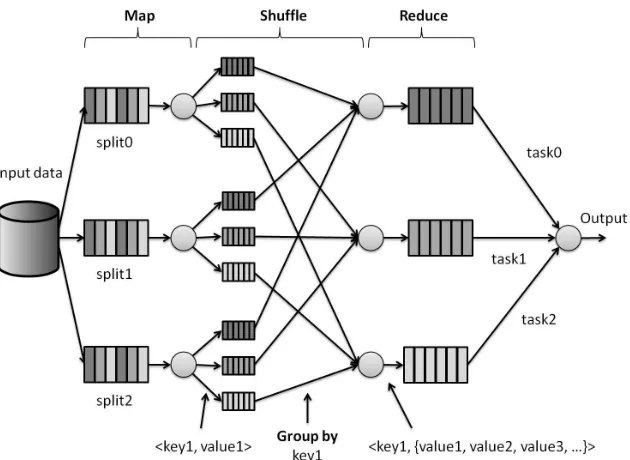
MapReduce [29, 36] is one of the most popular frameworks to deal with Big Data. This programming paradigm was proposed by Google in 2004 and designed for processing huge amounts of data over a cluster of machines. The MapReduce model is composed of two main phases: Map and Reduce. In general terms, the Map phase processes the input data set, producing some intermediate results. Then, the Reduce phase combines these intermediate results in some way to form the final output.
The MapReduce model is based on a basic data structure known as < key, value > pairs. In terms of the < key, value > pairs, in the first phase, the Map function receives a single< key, value >pair as input and generates a list of intermediate < key, value >pairs as output. This is represented by the form:
map(key1, value1)−→list(key2, value2) (1)
Between the Map and Reduce functions, the MapReduce library groups by key all intermediate < key, value > pairs. Finally, the Reduce function takes the intermediate < key, value > pairs previously aggregated by key and generates a new < key, value >pair as output. This is depicted by the form:
reduce(key2, list(value2))−→(key2, value3) (2)
Figure 2 depicts a flowchart of the MapReduce framework.
Figure 2: Flowchart of the MapReduce framework
< word,1>pairs by its corresponding word, creating a list of 1’s per word
< word, list(1′s) >. Finally, the reduce phase performs the sum of all the
1’s contained in the list of each word, providing the final count of repetition per word.
Apache Hadoop [37, 38] is the most popular implementation of the MapRe-duce programming model. It is an open-source framework written in Java supported by the Apache Software Foundation that allows the processing and management of large data sets in a distributed computing environment. In addition, Hadoop provides a distributed file system (HDFS) that replicates the data files in many storage nodes, facilitates rapid data transfer rates among those nodes and allows the system to continue operating without interruption when one node fails.
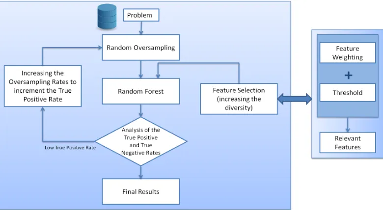
Figure 3: Flowchart of the procedure followed during the competition
among others.
4. The ROSEFW-RF algorithm to tackle an extremely imbalanced big data bioinformatics problem
In this section we explain in detail our ROSEFW-RF method as well as the partial experimental results that led us to select the specific algorithms (and adjust them) for each stage in the method. The description of the method is chronological: we describe the timeline of the method building process and what design decision were taken at each point of the process based on our successive experiments.
We have divided this section in five different steps that correspond to the main milestones (Section 4.1 to Section 4.5). Finally, Section 4.6 compares our performance to the results achieved by the rest of participants in the ECBDL’14 big data challenge.
4.1. Step 1: Balancing the data and Random Forest runs
This section is devoted to show the initial approach that we followed to deal with the proposed problem. Section 4.1.1 defines the models used and Section 4.1.2 is focused on the experimental results.
4.1.1. Description of the model
In [23], we conducted an extensive study to evaluate the performance of diverse approaches such as oversampling, undersampling and cost-sensitive learning for imbalance big data classification.
One of the outcomes of this extensive experimental evaluation was the observation that oversampling is more robust than undersampling or cost-sensitive approaches when increasing the number of maps. Therefore, despite the necessary increment on the data size produced by oversampling approach its use is preferred in large scale problems given that the additional cost it introduces can be compensated by the use of a larger number of maps. The dataset of the ECBDL’14 challenge is much larger than any of the datasets used in [23], hence we expected oversampling to perform better than under-sampling and cost-sensitive approaches, and indeed that was confirmed by our preliminary experiments comparing Random Oversampling (ROS) [11] to undersampling and cost-sensitive learning. Therefore, we will focus only on this class imbalance strategy for the rest of the paper.
ROS randomly replicates minority class instances from the original data set until the number of instances from the minority and majority classes is the same or a certain replication factor is reached.
We adapted this model to tackle big data using the MapReduce paral-lelization approach. Algorithms 1 and 2 present the pseudo-code of map and reduce phases, respectively. Specifically, each Map process is responsible for adjusting the class distribution in a mapper’s partition through the random replication of minority class instances. The Reduce process is responsible for collecting the outputs generated by each mapper to form a new balanced data set.
scat-tered the replicated minority instances through the different reducers that will write the final data set on disk.
The number of replicas of each instance is referred as thereplication f actor. For example, a replication factor of 1 means that there is only one copy of each instance in a mappers partition, a replication factor of 2 means two copies of each instance and so on. This replication factor is calculated with the total majority class instances and the total instances of the class of the instance that we want to replicate.
We would like to remark that the class distribution of the resulting dataset is not influenced by the number of maps used, and that in all cases the more mappers, the faster this stage will be.
Algorithm 1 Map phase for the ROS algorithm MAP(key, value):
Input: <key,value> pair, where key is the offset in bytes and value is the content of an instance.
Output: <key’,value’> pair, where key’ is any Long value and value’ is the content of an instance.
1: instance ←IN ST AN CE REP RESEN T AT ION(value) 2: class←instance.getClass()
3: replication f actor ←COM P U T E REP LICAT ION F ACT OR(class) 4: random←newRandom()
5: if class==majorityClass then
6: random value←random.nexInt(replication f actor) 7: key ←random value
8: EMIT (key, instance) 9: else
10: for i= 0 to replication f actor − 1 do
11: key ←i
12: EMIT (key, instance) 13: end for
14: end if
Algorithm 2 Reduce phase for the ROS algorithm REDUCE(key, values):
Input: <key,values> pair, where key is any Long value and values is the content of the instances.
Output: <key’,value’> pair, where key’ is a null value and value’ is the content of an instance.
1: while values.hasN ext() do
2: instance←values.getV alue() 3: EMIT (null, instance)
4: end while
Afterwards, we apply the RF algorithm to this data. To deal with big data experiments the original RF algorithm needs to be modified so it can effectively process all the data available. The Mahout Partial implementation (RF-BigData) [31] is an algorithm that builds multiple trees for different portions of the data. This algorithm is divided into two different phases: the first phase is based on the creation of the model (See Algorithm 3) and the second phase will estimate the classes associated with the data set using the previous learned model (See Algorithm 4).
Algorithm 3 Map phase for the RF-BigData algorithm for the building of the model phase MAP(key, value):
Input: <key,value> pair, where key is the offset in bytes and value is the content of a instance.
Output: <key’,value’> pair, where key’ indicates both the tree id and the data partition id used to grow the tree and value’ contains a tree. 1: instance ← IN ST AN CE REP RESEN T AT ION(value) {instances
will contain all instances in this mapper’s split} 2: instances←instances.add(instance)
{ CLEANUP phase: }
3: bagging←BAGGIN G(instances)
4: for i= 0 to number of trees to be built by this mapper − 1do
5: tree←bagging.build()
6: key ←key.set(partitionId, treeId) 7: EMIT (key, tree)
In the first stage, each Map task builds a subset of the forest with the data chunk of its partition and generates a file containing the built trees. Instructions 3-7 in Algorithm 3 detail how the bagging approach is applied on the data chunk corresponding to this map to build a set of trees. As a result of this phase, each tree is emitted together with its identifier (partitionId), as key-value pairs. Finally, all the solutions from the Map phase are stored. The second stage consists of the classification of the test set. The map phase will divide the test set in different subsets in which each mapper esti-mates the class for the examples available in it using a majority vote of the predicted class by the trees in the RF model built in the previous phase. As shown by Instructions 1-5 in Algorithm 4, the actual and predicted classes of all the instances are returned as key-value pairs. Finally, the predictions generated by each mapper are concatenated to form the final predictions file.
Algorithm 4 Map phase for the RF-BigData algorithm for classifying phase MAP(key, value):
Input: <key,value> pair, where key is the offset in bytes and value is the content of a instance.
Output: <key’,value’>pair, where key’ indicates the class of a instance and value’ contains its prediction.
1: instance ←IN ST AN CE REP RESEN T AT ION(value) 2: prediction←CLASSIF Y(instance)
3: lkey ←lkey.set(instance.getClass()) 4: lvalue←lvalue.set(prediction) 5: EMIT (lkey, lvalue)
Please note that neither stage has an explicit Reduce function, just Map-pers. More details about this algorithm can be found in [23].
4.1.2. Experiments
Since the application of the RF-BigData algorithm over the original data (without preprocessing) provided us totally biased results to the negative class, our initial aim was to check if the random oversampling approach allowed us to obtain similar TPR and TNR. We also wanted to analyze the influence of the number of mappers over the precision and the runtime needed.
Figure 4: Runtime vs. TPR·TNR
• Number of mappers: 64, 192 and 256.
• Number of used features per tree: log #F eatures + 1.
• Number of trees: 100.
[image:15.595.165.446.523.583.2]Table 1 collects the results of this initial experiment that uses a 100% of oversampling ratio and RF as classifier, showing the TPR, TNR and TPR · TNR. Figure 4 plots a comparison between the precision (in terms of TPR · TNR) and the runtime needed (in seconds) depending on the the number of Maps used.
Table 1: Results obtained by ROS (100%) + RF-BigData
Number of Maps TPR TNR TPR · TNR 64 0.564097 0.839304 0.473449 192 0.580217 0.821987 0.476931 256 0.579620 0.820509 0.475584
Our conclusions from this initial experiment are:
• Within the proposed parallel framework, the RF algorithm does not dispose of the full information about the whole addressed problem. Hence, it is expected that the precision obtained decreases according as the number of instances in the training set is reduced, that is, the number of maps is incremented. The variability of the TPR and TNR rates avoid to obtain higher TPR · TNR rates with a lesser number of mappers.
• In terms of runtime, as expected, we can observe a clear reduction as the number of mappers is increased. Note that due to the fact that we only disposed of 192 cores for our experiments, we could not expect an linear speed up when using more than 192 mappers.
In conclusion, the classifier kept biased to the negative class. Hence, the objective of our experiments is clear: to increase the TPR rate.
4.2. Step 2: Increasing the oversampling rates to increment the True Positive Rate
In order to bias our method towards the positive examples to further bal-ance TPR and TNR, we decided to augment the ratio of positive instbal-ances in the resulting preprocessed data set. To do this, we increment the over-sampling percentage in small steps from 100% to 130%. At this stage, we only focused on 64 and 192 mappers, and the parameters for RF-BigData were kept the same of the previous study.
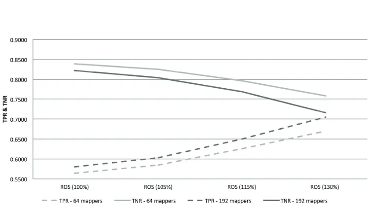
Table 2 presents the results obtained with the idea of increasing the over-sampling ratio. Figure 5 shows how the TPR and TNR rates vary depending on the oversampling rate and the number of mappers.
The conclusions of this second round of experiments were:
• The increment of the oversampling rate has played an important role to find out a balance between the TPR and TNR rates that results in a higher precision (TPR · TNR). This behavior has been produced independently on the number of mappers used. Nevertheless, with a reduced number of mappers (64) we still obtained greater differences between the TPR and the TNR in comparison to the results obtained with 192 mappers.
Table 2: Results obtained with different ROS oversampling rates
Oversampling Ratio Number of Maps TPR TNR TPR · TNR 100% 64 0.564097 0.839304 0.473449
192 0.580217 0.821987 0.476931 105% 64 0.585336 0.824809 0.482791 192 0.603388 0.803819 0.485015 115% 64 0.626581 0.796581 0.499122 192 0.650081 0.768483 0.499576 130% 64 0.670189 0.758622 0.508420
192 0.704772 0.716172 0.504738
[image:17.595.119.494.382.594.2]summary, the higher ROS percentage, the higher TPR and the lower TNR.
4.3. Step 3: Detecting relevant features via evolutionary featuring weighting
This section presents the second preprocessing component we decided to use in order to improve the overall precision. Section 4.3.1 describes the proposed preprocessing techniques and Section 4.3.2 shows the experimental results.
4.3.1. Description of the model
Since the ECBDL’14 data set contains a fairly large number of features (631), we decided to include a new preprocessing component to our model that allowed us to consider the relevance of the features. We aimed at elimi-nating redundant, irrelevant or noisy features by computing the importance of them in terms of weights.
To do so, we focused on the evolutionary approach for Feature Weighting (FW) proposed in [30] called “Differential Evolution for Feature Weighting” (DEFW). FW can be viewed as a continuous space search problem in which we want to determine the most appropriate weights for each feature. The DEFW method is based on a self-adaptive differential evolution algorithm [39] to obtain the best weights.
DEFW starts with a population of individuals. Each one encodes a weight vectorW eights[1..D] = (W1, W2, ..., WD), whereDis the number of features,
which is a weight for each feature of the problem, that are initialized ran-domly within the range [0,1]. DEFW enters in a loop in which mutation and crossover operators generate new potential solutions. Finally, the selection operator must decide which generated trial vectors should survive in the pop-ulation of the next generation. The Nearest Neighbor rule [40] was used to guide this operator. To implement a self-adaptive DE scheme, independent of configuration parameters, DEFW uses the ideas established in [41].
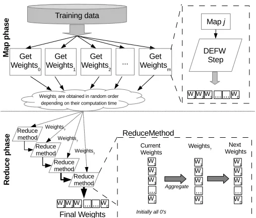
As such, this method is unable to deal with big data problems. To the best of our knowledge, there is no any proposed approach to enable evolutionary FW algorithms to address these volumes of data. Therefore, we developed a MapReduce Approach for FW. Algorithms 5 and 6 detail the map and reduce operations, respectively.
will perform a whole evolutionary FW cycle. That is, a complete loop of mutation, crossover and selection operators for a given number of iterations. To do so, we use the DEFW method over the given subset of examples (Instruction 3 in Algorithm 5). The configuration parameters used are: iterations = 500, iterSFGSS = 8, iterSFHC =20, Fl=0.1 and Fu=0.9. Please note that the different mapper instances, although they are applied with data partitions of similar volume, may have varying runtimes. The MapReduce framework starts the reduce phase as the first mapper has finished its computation. It will emit a resulting vector of weights W eightsj[1..D], measuring the importance of each feature
regarding this subset of the whole training set.
• The reduce phase will consist of the iterative aggregation of all the
W eightsj[1..D], provided by the maps, as a single one W eights.
Ini-tially the Weights of every feature are established to 0,W eights[1..D] = {0,0, ...,0}. As the maps finish their computation, the W eights[1..D] variable will sum the feature importance obtained in each map with the current Weights (Instruction 6 in Algorithm 6). The proposed scheme only uses one single reducer that is run every time that a mapper is completed. With the adopted strategy, the use of a single reducer is computationally less expensive than use more than one. It decreases the Mapreduce overhead (especially network overhead) [42, 43].
• At the end of the reduce phase, the resulting W eights will be used together with a threshold Tf to select those characteristics that have
been ranked as the most important ones.
Figure 6 illustrates the MapReduce process for FW, differentiating be-tween the map and reduce phases. It puts emphasis on how the single reducer works and it forms the final W eightsvector.
4.3.2. Experiments
Algorithm 5 Map phase for the DEFW algorithm MAP(key, value):
Input: <key,value> pair, where key is the offset in bytes and value is the content of a instance.
Output: <key’,value’> pair, where key’ indicates the data partition id (partitionId) used to perform the DEFW and value’ contains the pre-dicted W eightsj[1..D].
1: instance ←IN ST AN CE REP RESEN T AT ION(value) 2: instances←instances.add(instance)
{ CLEANUP phase: }
3: W eightsj[1..D]=DEF W(instances)
4: lkey ←lkey.set(partitionId)
5: lvalue←lvalue.set(W eightsj[1..D])
6: EMIT (lkey, lvalue)
Algorithm 6 Reduce phase for the DEFW algorithm MAP(key, value):
Input: <key,value>pair, where key is the data partition id used in the Map Phase and value is the content of a W eightj[1..D] vector.
Output: <key’,value’> pair, where where key’ is a null value and value’ is the resulting feature W eights[1..D] vector.
1: instance ←IN ST AN CE REP RESEN T AT ION(value) 2: {Initially W eights[1..D] = 0,0, ...,0}
3: while values.hasN ext() do
4: W eightsj[1..D] =values.getV alue()
5: for i= 1 to D do
6: W eights[i] =W eights[i] +W eightsj[i]
7: end for
8: end while
Figure 6: MapReduce Feature Weighting scheme
time restrictions, we did not investigate further the influence of the number of maps in the quality of the selected features.
After the FW process we ranked the features by weight and selected a feature subset of highly ranked features. We performed preliminary experi-ments (not reported) to choose the most suitable selection threshold. From the original 631 features we only kept the subset of 90 features with the highest weights.
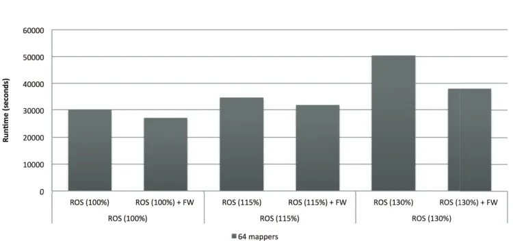
With the selected features, we repeated the experiment using the over-sampling+RF approach with an oversampling ratio ranging from 100% to 130%. Table 3 shows the results obtained. Figure 7 compares the runtime needed to perform the building of the RF classifier by using the original set of features and using the 90 selected characteristics.
From this third stage of experiments we concluded that:
• The use of DEFW showed to provide a greater precision compared to the previous results. Using a smaller set of features than before, the RF-BigData model has been able to increase its performance.
Table 3: Results obtained with the subset of 90 features provided by the FW method
Oversampling Ratio Number of Maps TPR TNR TPR · TNR 100% 64 0.593334 0.837520 0.496929
192 0.610626 0.818666 0.499899 115% 64 0.641734 0.804351 0.516179 192 0.661616 0.778206 0.514873 130% 64 0.674754 0.777440 0.524580
192 0.698542 0.746241 0.521281
Best result from the previous stages 0.670189 0.758622 0.508420
[image:22.595.120.495.407.583.2]has mainly increased the performance in the TPR, but also we improve the classification done in the negative class. However, we observed differences between the TPR and the TNR rates even using 130% of oversampling percentage. Should we increment more the oversampling rate to balance the precision obtained in both classes? (see Section 4.5).
• In terms of runtime, the reduction of the number of features has shown a notable reduction of the time requirements due to the reduction of the size of the problem.
Hence, the introduction of feature selection has resulting in a large leap forward in the performance of our algorithm.
4.4. Step 4: Investigating RF parameters
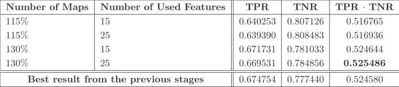
[image:23.595.114.504.471.556.2]Due to the lack of balance between the TPR and TNR of our method, even in the best performing variants, we decided to investigate the influence of internal number of features used by RF. We focused on the best two oversampling ratios from the previous section and we increment the number of features used. Instead of using the log #F eatures + 1, that resulted in 8 features, we incremented to 15 and 25. Table 4 presents the results of this experiment.
Table 4: Results obtained varying the number of internal feature used by RF
Number of Maps Number of Used Features TPR TNR TPR ·TNR
115% 15 0.640253 0.807126 0.516765
115% 25 0.639390 0.808483 0.516936
130% 15 0.671731 0.781033 0.524644
130% 25 0.669531 0.784856 0.525486
Best result from the previous stages 0.674754 0.777440 0.524580
4.5. Step 5: Combining ROS with very large oversampling rates and feature weighting
Our previous steps produced successful improvements in the precision of the model. However, we again get high differences among the precision obtained in the positive and the negative classes. In order to mitigate this issue, we came back to the solution adopted in the Step 2 (Section 4.2), increasing the ROS rate.
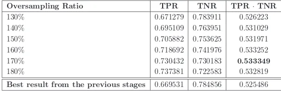
[image:24.595.164.444.364.455.2]In this last stage of experiments we focused on the specific configuration that had obtained the best performance up to that point: 64 mappers, 90 fea-tures selected by the FW model and 25 internal feature for RF. Afterwards, we increased the ROS ratio until the TPR was larger than the TNR. Table 5 collects the results of this experiment and Figure 8 plots the evolution of TPR and TNR when the oversampling ratio is augmented.
Table 5: Result obtained with huge ROS oversampling rates: 64 mappers, 90 features, and 25 internal features for RF
Oversampling Ratio TPR TNR TPR·TNR
130% 0.671279 0.783911 0.526223
140% 0.695109 0.763951 0.531029
150% 0.705882 0.753625 0.531971
160% 0.718692 0.741976 0.533252
170% 0.730432 0.730183 0.533349
180% 0.737381 0.722583 0.532819
Best result from the previous stages 0.669531 0.784856 0.525486
In conclusion, we observe that we needed a huge oversampling rate of 170% to balance the TPR and TNR rates. This increment in conjunc-tion with all the previous steps generated the best overall submission of the ECBDL’14 big data challenge.
4.6. Comparison with the rest of the methods
In this section we collect the best results achieved from the Top 5 partic-ipants of the competition to merely compare the precision obtained. Table 6 presents these final results. A brief description of each method as well as a qualitative runtime comparison between them, based on participant’s self-reported information, is available at http://cruncher.ncl.ac.uk/bdcomp/
BDCOMP-final.pdf. Moreover, the timeline and ranking of the prediction
Figure 8: TPR vs. TNR varying the ROS percentage
Table 6: Comparison with the rest of the participants
Team TPR TNR TPR · TNR
Efdamis 0.730432 0.730183 0.533349
ICOS 0.703210 0.730155 0.513452
UNSW 0.699159 0.727631 0.508730
HyperEns 0.640027 0.763378 0.488583
[image:25.595.171.447.536.634.2]This table reflects the difficulties that this bioinformatics problem has brought to most of the contestants. We can observe that find a balance between the TPR and TNR rates has been the main barrier for all of the participants of the competition.
5. Conclusions
In this work we have presented the winner algorithm of the ECBDL’14 data mining competition, called ROSEFW-RF. We have dealt with an im-balance bioinformatics big data application with different learning strategies. We have combined several preprocessing stages such as random oversampling and evolutionary feature weighting before building a learning model. All of our approaches have been based on MapReduce as parallelization strategy.
In this particular problem, the necessity of balancing the TPR and TNR ratios emerged as a difficult challenge for most of the participants of the competition. In this sense, the results of the competition have shown the goodness of the proposed MapReduce methodology. Particularly, our modu-lar ROSEFW-RF methodology composed of several, highly scalable, prepro-cessing and mining methods has shown to be very successful in this challenge and outperform the other participants.
As future work, we would like to further investigate the proposed evolu-tionary feature selection approach, by analyzing the influence of the number of maps and other base classifiers. Moreover, the development of mixed strategies between undersampling and oversampling approaches or instance reduction techniques (such as [43]) may also boost the classification perfor-mance in imbalanced big data problems.
Acknowledgment
Supported by the Research Projects TIN2011-28488, P10-TIC-6858 and P11-TIC-7765. I. Triguero holds a BOF postdoctoral fellowship from the Ghent University.
Appendix A. Hardware and Software tools
• Processors: 2 x Intel Xeon CPU E5-2620
• Cores: 6 per processor (12 threads)
• Clock Speed: 2.00 GHz
• Cache: 15 MB
• Network: Gigabit Ethernet (1 Gbps)
• Hard drive: 2 TB
• RAM: 64 GB
The master node works as the user interface and hosts both Hadoop mas-ter processes: the NameNode and the JobTracker. The NameNode handles the HDFS, coordinating the slave machines by the means of their respective DataNode processes, keeping track of the files and the replications of each HDFS block. The JobTracker is the MapReduce framework master process that manages the TaskTrackers of each compute node. Its responsibilities are maintaining the load-balance and the fault-tolerance in the system, ensuring that all nodes get their part of the input data chunk and reassigning the parts that could not be executed.
The specific details of the software used are the following:
• MapReduce implementation: Hadoop 2.0.0-cdh4.4.0. MapReduce 1 runtime(Classic). Cloudera’s open-source Apache Hadoop distribu-tion [44].
• Maximum maps tasks: 192.
• Maximum reducer tasks: 1.
• Machine learning library: Mahout 0.8.
• Operating system: Cent OS 6.4.
References
[1] E. Alpaydin, Introduction to Machine Learning, 2nd Edition, MIT Press, Cambridge, MA, 2010.
[2] F. Zhang, J. Y. Chen, Data mining methods in omics-based biomarker discovery, in: Bioinformatics for Omics Data, Springer, 2011, pp. 511– 526.
[3] H. Mamitsuka, M. Kanehisa, Data Mining for Systems Biology, Springer, 2013.
[4] J. Bacardit, P. Widera, N. Lazzarini, N. Krasnogor, Hard data analytics problems make for better data analysis algorithms: Bioinformatics as an example, Big data 2 (3) (2014) 164–176.
[5] P. Larraaga, B. Calvo, R. Santana, C. Bielza, J. Galdiano, I. Inza, J. A. Lozano, R. Armaanzas, G. Santaf, A. Prez, V. Robles, Machine learning in bioinformatics, Briefings in Bioinformatics 7 (1) (2006) 86–112.
[6] I. T. Jolliffe, Principal Component Analysis, Springer-Verlag, Berlin; New York, 1986.
[7] Y. Saeys, I. Inza, P. Larra˜naga, A review of feature selection techniques in bioinformatics, Bioinformatics 23 (19) (2007) 2507–2517.
[8] V. L´opez, A. Fern´andez, S. Garc´ıa, V. Palade, F. Herrera, An insight into classification with imbalanced data: Empirical results and cur-rent trends on using data intrinsic characteristics, Information Sciences 250 (0) (2013) 113 – 141.
[9] R. Blagus, L. Lusa, Class prediction for high-dimensional class-imbalanced data, BMC Bioinformatics 11 (1) (2010) 523.
[10] R. Blagus, L. Lusa, Smote for high-dimensional class-imbalanced data, BMC Bioinformatics 14 (1) (2013) 106.
[12] A. Fern´andez, S. R´ıo, V. L´opez, A. Bawakid, M. del Jesus, J. Ben´ıtez, F. Herrera, Big data with cloud computing: An insight on the computing environment, mapreduce and programming frameworks, WIREs Data Mining and Knowledge Discovery 4 (5) (2014) 380–409.
[13] X. Wu, X. Zhu, G. Wu, W. Ding, Data mining with big data, IEEE Transactions on Knowledge and Data Engineering 26 (1) (2014) 97–107.
[14] I. Palit, C. Reddy, Scalable and parallel boosting with mapreduce, IEEE Transactions on Knowledge and Data Engineering 24 (10) (2012) 1904– 1916.
[15] G. Caruana, M. Li, Y. Liu, An ontology enhanced parallel SVM for scalable spam filter training, Neurocomputing 108 (0) (2013) 45 – 57.
[16] A. Haque, B. Parker, L. Khan, B. Thuraisingham, Evolving big data stream classification with mapreduce, in: Cloud Computing (CLOUD), 2014 IEEE 7th International Conference on, 2014, pp. 570– 577. doi:10.1109/CLOUD.2014.82.
[17] C. P. Chen, C. Zhang, Data-intensive applications, challenges, tech-niques and technologies: A survey on big data, Information Sciences 275 (2014) 314–347.
[18] K. Kambatla, G. Kollias, V. Kumar, A. Grama, Trends in big data an-alytics, Journal of Parallel and Distributed Computing 74 (2014) 2561– 2573.
[19] M. Galar, A. Fern´andez, E. Barrenechea, H. Bustince, F. Herrera, A re-view on ensembles for the class imbalance problem: Bagging-, boosting-, and hybrid-based approaches, IEEE Transactions on Systems, Man, and Cybernetics, Part C: Applications and Reviews 42 (4) (2012) 463–484.
[20] B. Krawczyk, M. Wozniak, B. Cyganek, Clustering-based ensembles for one-class classification, Information Sciences 264 (0) (2014) 182 – 195. doi:http://dx.doi.org/10.1016/j.ins.2013.12.019.
[21] L. Breiman, Random forests, Machine Learning 45 (1) (2001) 5–32.
[23] S. del R´ıo, V. L´opez, J. M. Ben´ıtez, F. Herrera, On the use of mapre-duce for imbalanced big data using random forest, Information Sciences 285 (0) (2014) 112–137.
[24] G. D. F. Morales, A. Bifet, D. Marron, Random forests of very fast deci-sion trees on gpu for mining evolving big data streams, in: Proceedings of ECAI 2014, 2014, pp. 615–620.
[25] Evolutionary computation for big data and big learning workshop. data mining competition 2014: Self-deployment track (2014).
URL http://cruncher.ncl.ac.uk/bdcomp/
[26] J. Bacardit, P. Widera, A. Marquez-Chamorro, F. Divina, J. S. Aguilar-Ruiz, N. Krasnogor, Contact map prediction using a large-scale ensem-ble of rule sets and the fusion of multiple predicted structural features, Bioinformatics 28 (19) (2012) 2441–2448.
[27] M. Punta, B. Rost, Profcon: novel prediction of long-range contacts, Bioinformatics 21 (13) (2005) 2960–2968.
[28] J. Cheng, P. Baldi, Improved residue contact prediction using support vector machines and a large feature set, BMC Bioinformatics 8 (1).
[29] J. Dean, S. Ghemawat, Mapreduce: simplified data processing on large clusters, Communications of the ACM 51 (1) (2008) 107–113.
[30] I. Triguero, J. Derrac, S. Garc´ıa, F. Herrera, Integrating a differential evolution feature weighting scheme into prototype generation, Neuro-computing 97 (0) (2012) 332 – 343.
[31] A. M. Project, Apache mahout (2013).
URL http://mahout.apache.org/
[32] D. Jones, Protein secondary structure prediction based on position-specific scoring matrices, J Mol Biol 292 (1999) 195–202.
[34] M. Stout, J. Bacardit, J. D. Hirst, N. Krasnogor, Prediction of recursive convex hull class assignments for protein residues, Bioinformatics 24 (7) (2008) 916–923.
[35] B. Monastyrskyy, K. Fidelis, A. Tramontano, A. Kryshtafovych, Evalu-ation of residue-residue contact predictions in CASP9, Proteins: Struc-ture, Function, and Bioinformatics 79 (S10) (2011) 119–125.
[36] J. Dean, S. Ghemawat, Map reduce: A flexible data processing tool, Communications of the ACM 53 (1) (2010) 72–77.
[37] T. White, Hadoop: The Definitive Guide, 3rd Edition, O’Reilly Media, Inc., 2012.
[38] A. H. Project, Apache hadoop (2013).
URL http://hadoop.apache.org/
[39] S. Das, P. Suganthan, Differential evolution: A survey of the state-of-the-art, IEEE Transactions on Evolutionary Computation 15 (1) (2011) 4–31.
[40] T. M. Cover, P. E. Hart, Nearest neighbor pattern classification, IEEE Transactions on Information Theory 13 (1) (1967) 21–27.
[41] F. Neri, V. Tirronen, Scale factor local search in differential evolution, Memetic Computing 1 (2) (2009) 153–171.
[42] C.-T. Chu, S. Kim, Y.-A. Lin, Y. Yu, G. Bradski, A. Ng, K. Olukotun, Map-reduce for machine learning on multicore, in: Advances in Neural Information Processing Systems, 2007, pp. 281–288.
[43] I. Triguero, D. Peralta, J. Bacardit, S. Garc´ıa, F. Herrera, MRPR: A mapreduce solution for prototype reduction in big data classification, Neurocomputing 150 (20) (2015) 331–345.
[44] Cloudera, Cloudera distribution including apache hadoop (2013).