Mutation models and quantitative genetic variation.

(1)

Mutation Models and Quantitative Genetic Variation

Zhao-Bang

Zeng

and C. Clark Cockerham

Program in Statistical Genetics, Department of Statistics, North Carolina State University, Raleigh, North Carolina 27695-8203 Manuscript received August 3 1, 1992

Accepted for publication November 20, 1992

ABSTRACT

Analyses of evolution and maintenance of quantitative genetic variation depend on the mutation models assumed. Currently two polygenic mutation models have been used in theoretical analyses. One is the random walk mutation model and the other is the house-of-cards mutation model. Although in the short term the two models give similar results for the evolution of neutral genetic variation within and between populations, the predictions of the changes of the variation are qualitatively different in the long term. In this paper a more general mutation model, called the regression mutation model, is proposed to bridge the gap of the two models. The model regards the regression coefficient, 7 , of the effect of an allele after mutation on the effect of the allele before mutation as a parameter. When y = 1 or 0, the model becomes the random walk model or the house-of-cards model, respectively. The additive genetic variances within and between populations are formulated for this mutation model, and some insights are gained by looking at the changes of the genetic variances as 7 changes. The effects of 7 on the statistical test of selection for quantitative characters during macroevolution are also discussed. T h e results suggest that the random walk mutation model should not be interpreted as a null hypothesis of neutrality for testing against alternative hypotheses of selection during macroevolution because

_-

it can potentially allocate too much variation for the change of population means under neutrality.

T

HERE has been considerable interest in recent years in developing neutral theories of phenotypic evolution as a null hypothesis for testing for significance of other evolutionary forces such as selection, or as a basis for estimating genetic parameters such as the rate of new genetic variance entering a population via mutation. Developing a neutral theory is essential for us to understand the mechanisms and processes of evolution. But it is important to realize that the construction of the null hypothesis of neutrality depends on the mutation model assumed.

T h e most general mutation model for arbitrary

k

alleles is that the mutation rate from allele A, t o allele

A, is simply denoted by uy. With different specifica- tions for uy, the model can be used to analyze different situations. This general model is however usually not manageable. Instead, for many genetic analyses, sim-

plified mutation models are used, among them two

extreme polygenic mutation models have been used extensively in recent theoretical analyses. O n e is t h e random walk mutation model which was first used by

CLAYTON a n d ROBERTSON (1955) as an approximation, later explicitly proposed by CROW a n d KIMURA (1964) and KIMURA (1965), and subsequently pop-

ularized by LANDE (1975). This model assumes that each mutation yields a new allele (an infinite allele model) and that mutation transforms an allele of effect x into an allele of effect x ’ with

x ’ = x + [ (1)

Genetics 133: 729-736 (March, 1993)

where [ is a random variable defined by the density functionf([) with mean zero and variance a:. In this case the rate of mutation from an allele with effect xi

t o a n allele with effect x, is specified by u g = uf([)d[ where [ = xj

-

xi, f ( [ ) d [ specifies the probability of finding [ in the range ([,[

+

d [ ) a n d u is the mutation rate. Because mutation does not change the mean of allelic effects and the increase of the genetic variance is expected to be constant, the model is also called t h e constant variance model. This model has the appeal of relating various evolutionary quantities to the pa-

(2)

T h e other model is the house-of-cards mutation model which was formally proposed and introduced

by KINGMAN (1977, 1978) and had been used previ-

ously as a simplification in several studies by WRIGHT

( 1 948, p. 1 14; 1969, p. 394), WATTERSON ( 1 977) and LI ( 1 977). For

k

finite alleles, the model assumes that

u g = uj for all i # j and for infinite alleles the model is equivalent to assuming that mutation transforms an allele of effect x into an allele of effect x ’ with

x ) = [ (2)

so that “the fitness of the mutant is chosen at random

from a fixed fitness distribution” (KINGMAN, 1977, p.

451). Note that [ in (2) does not have to have the

same distribution as [ in (1). But for the convenience

of comparison it is assumed in this study that [ in (2)

has the same distribution as that of [ in ( 1 ) . Thus, in this model uy = uf(xj)dxj = uj since xj =

[.

It has been

acknowledged that the model is “crude in the ex-

treme” and has severe restrictions. In contrast with the random walk mutation model, this model behaves

properly in different time horizons. By using this

mutation model, COCKERHAM and TACHIDA (1987)

observed that, without selection, the between-population genetic variance does not increase indefinitely, but goes to a finite equilibrium value, which is in sharp

contrast to the analyses of CHAKRABORTY and NEI

(1 982) and LYNCH and HILL (1 986). There will also

be a limit to response to directional selection and

mutation under this mutation model (ZENG, TACHIDA

and COCKERHAM 1989). It has been criticized that this

model assumes that any allele can be obtained by a

single step mutation from any other allele. If however,

we consider the case of infinite alleles, the issue is the relationship between the effects of alleles before

and after mutation; that is, whether the effect of a

mutant depends on the effect of its parent allele. This

relationship is of course not known. As expressed by

OHTA and TACHIDA (1 990), the two models, proposed

for mathematical tractability, may represent two extremes between which the real situation may lie.

T o bridge the gap of the two models and to unify and reconcile previous analyses, we introduce a new

mutation model in this paper which takes the regres-

sion coefficient, y, of the effect of a mutant on the

effect of its parent allele as a parameter. More specif-

ically we assume

x ’ = y x + [ 0 5 y l l . (3)

In this case it is assumed that u g = uf ( x j

-

yxi)d(xj

-

yxi). When y = 1 or 0, this represents the random walk model or the house-of-cards model, and the two

models are then bridged by the parameter 7. when 0

<

y

<

1, the model will impose an upper bound on the genetic variance accessible by mutation at a locus, and at the same time will also impose some restrictions

on the availability of allelic effects accessible in a single

step of mutation. This model may be called the regres-

sion mutation model as it depends on the parameter

7. Although this mutation model is relatively more

general than the random walk model and the house- of-cards model, the model is not a general mutation

model in the sense that u g is specified by a fixed

function.

Sometimes we are interested in the relationship between the change of allelic effect by mutation and

the effect of the allele before mutation. By (3), this

relation is defined as

6x = X I

-

x = (y

-

1)x

+

[

and (y

-

1 ) is the regression coefficient of 6x on x.

This regression coefficient is 0 under the random

walk mutation model and -1 under the house-of-cards

mutation model.

By using this mutation model, we will analyze the genetic variances within and between populations, and

show how the variances change as y changes and how

the value of y influences the estimation of genetic

parameters, such as V,. We will also show how the

test for selection on the rate of phenotypic evolution depends on the mutation models assumed.

THE REGRESSION MUTATION MODEL

T h e model defined by (3) describes a process which

is similar to the Ornstein-Uhlenbeck process (KARLIN

and TAYLOR 1981). Well known in physics, the Orn-

stein-Uhlenbeck process describes a particle executing Brownian motion while being coupled to the origin

by a weak spring as it models directly the velocity of

motion of a particle that has momentum but is subject to friction, which always tends to reduce the velocity toward zero. However, as we intend to analyze model

(3) for varying from 0 to 1, the spring in our model

can be weak or strong.

Why do we need such a regression mutation model? What plays the role of the spring for polygenic mutations? Because individual effects of polygenic mutations are generally undetectable, the genetic nature of polygenic mut2;ions is little understood. However,

no matter what causes it, it is clear that for fitness and

fitness related traits, the regression effects of new

mutants are apparent and are reflected by the tend-

ency that most mutations are deleterious (MUKAI

1964; MUKAI et al. 1972). This may be explained by the fact that these traits are under constant natural directional selection and the effects of alleles are al- ready at extremes.

(3)

directly or indirectly so that the traits are mostly at

intermediate levels which may make the regression

effects of mutants undetectable. There have been

some observations that mutations with relatively small effects on these kinds of quantitative traits arise in a nondirectional manner, having little average effect on

the mean of a character in an unselected base popu-

lation (OKA, HAYASHI and SHIOJIRI 1958; GREGORY

1965; MACKAY, LYMAN and JACKSON 1991). This,

however, does not necessarily support the random

walk mutation model, because the experimental base populations are not at extremes.

When the alleles express deleterious effects, it may well be appropriate to take both the effects of mutants on the quantitative character and fitness into account

and model them jointly [e.g., KEIGHTLEY and HILL

(1990)l. However, even if the alleles are strictly neutral, the changes of allelic effects due to mutation on the quantitative characters are not necessarily independent of their parent alleles. T h e phenotypic space of characters is not unbounded. Genes expressing their effects are subject to a lot of biological con-

straints including gene regulations, metabolic controls

and physiological constraints. All these constraints could play the role of the spring, weak or strong, like friction in physics. As an approximation, the regres-

sion model does appear to be more plausible (and

more general) than the pure random walk model and the house-of-cards model in modeling polygenic mu-

tations. T h e parameter y may then be viewed as a

measure of “intrinsic constraint,” although the exact relation between these constraints and the parameter is unclear.

T h e model defined by (3), though more compli-

cated than the random walk model, is mathematically

tractable. Several interesting genetic quantities can be

readily derived for the regression mutation model. Let us first analyze some basic genetic properties of the model for an infinite population. Let the effect of

an allele at generation t be xt. In each generation we

assume that mutation occurs at the rate of u and

whenever mutation occurs it introduces a new allele

into the population with an effect defined by (3). Then

at the t

+

1 generation

Xf+1 =

{&

v = { 1 with probability u

yxf

+

[ with probability u

with probability 1 - u.

This can be expressed as

x4+1 = (1

-

v)xt

+

v(yxf

+

l )

(4)

where

0 with probability 1

-

u

is an indicator variable having the expectation %’(v) =

.!i6’(v2) = u, where %’denotes expectation. By taking

the expectations with respect to v and [ ( k ,

9([)

=

0 and

9([’)

= u:) in (4), we then have

- ! q X f + l ) = P.!i6‘(Xd ( 5 )

%’(X?+l) = 7].!i6’(x:)

+

ua: (6)

where p = 1

-

u( 1

-

y) and TJ = 1

-

u(1

-

y2), and in

general

S ( X t ) = pf%’(xo)

(7)

(8) 2

kqx:) = s f 9 ( x ! )

+

(1

-

sf)

m.

UX

So the genetic variance at the tth generation is

Var(xt) = %’(x:)

-

[ 9 ( x t ) ] *

2

= sVar(x0)

+ ( 1

-

s?

”q

u x (9)

+

(11’

-

P2?[%’(XO)l2.

.!i6’(xtxs) = p .!i6’(Xtxs-l)

Furthermore, since

the covariance between xt and xs for t

<

s is

COV(Xt,XJ = %’(xlxJ

-

% ‘ ( X t ) . ! i 6 ’ ( 4 ( 1 0 )

= ps-‘Var(xf).

Ultimately, the genetic variance at a haploid locus is

u:/( 1

-

y2), which is infinite when y = 1, and a: when y = 0.

GENETIC VARIANCE WITHIN POPULATIONS

COCKERHAM and TACHIDA (1987) and LYNCH and

HILL (1 986), among others, have analyzed the genetic

variances within and between finite populations for the house-of-cards mutation model and random walk mutation model, respectively. T h e differences on the variances by the two models were discussed by C. C. COCKERHAM (unpublished data). As the regression mutation model tends to be more general and provides a means to bridge the gap of the two models, it would be interesting to see how the variances change

as y changes.

Following COCKERHAM and TACHIDA (1987), we

consider independent replicate random mating mon-

oecious diploid populations, each consisting of N in-

dividuals, all stemming from the same founder population. Only additive effects of alleles within and between loci are considered. We analyze the variances for a locus and the summation of the quantities over loci is implied. For a particular locus let the genotypic

value for a genotype with alleles Ai and A, be

G..

= x.

+

x .

’I

’

I ’

(4)

u w = 9 G 2

-

S G G '

where G and G ' are for a random pair of individuals

in the same populations. By definition

S G 2 = %'(xi

+

xj)'

= 29(x')

+

289(XiX!)

+

2( 1

-

e ) 9 ( x i x j ' )

.!i+?GG' = %'(x;

+

xj)(x;

+

x i )

= 4 0 9 ( ~ i ~ ! )

+

4( 1

-

I 3 ) 9 ( ~ i ~ j l )

where I3 is the coancestry coefficient between individ-

uals in the same populations which is the same as the inbreeding coefficient between two genes within an

individual, %'(x:) is the expected value of square of

the effect of a gene, %'(xixi) is the expected value of

product of two genes with the same effect and

g ( x i x ; ) is the expected value of product of two genes with different effects.

To derive the variance within populations, we need

to analyze the dynamic expectations of the above three

quantities and also I3 the coancestry coefficient.

Instead of analyzing the four quantities separately, however, we derive the transition equations for

three quantities: A = 9 ( x ? ) , B = 1 3 S ( x i x ; ) and C = (1

-

I3)9(xixj'), i.e., the expected values of allelic effects times the probability that genes are alike or not alike. For infinite alleles the probability of genes being alike is the same as for identity by descent. First, we observe

that sampling does not influence A, and

A, = [ l

-

~ ( l

-

y2)]A,-1

+

U U ~ (1 1)

as given by (6). For B f , we note that with probability 1/(2N), the two genes sampled are from the same gene with the expected value At, and with the remain-

ing probability 1

-

1/(2N), the two genes sampled are

from different genes, but were alike in the last gen-

eration with the expected value Bt-l and neither gene

having mutated with probability (1

-

u)'. Thus

Finally, for Cf, the two genes sampled must be from

different genes. Depending on whether the two genes

were alike or not alike in the last generation, there are two cases. They can be either alike in the last generation with either one or both genes having mu-

tated, which has the expected value [2u(l

-

u)y

+

u ~ ~ * ] B , - ~ , or not alike in the last generation, which has the expected value [ 1

-

u( 1

-

y)]'C,-l (with genes having or having not mutated). Thus

+

[ l - u(1

-

y)]2C,-,j.

~I

These lead to

+

1

--

([(l -u(1

-

7 2 ) )

(

4

- (1

-

U ( 1

-

y))2]2A,-1

+

ZUU:).

By using (8) and keeping terms of the order of Nu, the variance is then

u;, = X'U;,

+

(1

-

Xf)u;,

+

(7'

-

A')A (1 5 )

where 71 = 1

-

u(1

-

y2), X = (1

-

1/2N)[ 1

-

u( 1

-

r)]', a,,2 1s . the initial genetic variance,

is the equilibrium genetic variance, and

is a transient part of the genetic variance which depends on the initial state of the population. When

Y

= 0,

r

+

1

1 -

[(

1" 'i!N)(l

-

u)2]'

1

SNuu,'

1

+

4Nu

+[(l -+[(l -&)(l

4Nu[ g ( x f )

-

a:]

1

+

2Nu

which agrees with the result of COCKERHAM and

TACHIDA (1 987), and when y = 1

& = ( I - $ ) u & + [ l - ( I -$)]4Nuu;

which agrees with the result of LYNCH and HILL

(1 986).

Interestingly, at equilibrium

0;" =

{

4Nuu:

when y = 1

8Nuu:/( 1

+

4Nu) when y = 0.

This means that when 4Nu is less than 1, the equilib-

rium genetic variance with y = 0 is larger than that

with y = 1 and vice versa. However, note that this

behavior is a consequence of the assumption that [ in

(5)

informative for comparison for different mutation

models to have the variances standardized by the expected genetic variance after one generation mutation from an initially fixed population.

A fundamental parameter in quantitative genetics

is the increase of genetic variance by mutation in the first generation with the initial population fixed. This

parameter is denoted as V,,, in LYNCH and HILL (1 986)

and V, by C. C. COCKERHAM (unpublished data). When

y = 1, this is 2ua;. When y

<

1, however, this depends

on the initial state of the population. COCKERHAM and

TACHIDA (1 987) considered the case that the founder

population is randomly fixed with respect to the equilibrium distribution of allelic effects. This assumes

that A0 = a;/(1

-

7') and thus A = 0. With this

assumption

and

u2, = (1

-

Af)a:,.

In this paper we denote

4ua:

Vu = a:, =

-

1

+ Y

and V, = 2uu:.

Thus V, = V, when = 1. T h e ratio of the equilibrium

genetic variance to the increment of the variance in the first generation is then

2

a w *

-

2N

"

a:, 1

+

NU( 1

-

7)'

Unless y = 1, this ratio is less than 2N. When 4Nu is

small, the effect of y on the ratio is negligible. T h e

patterns of changes of a:J(2NV,) over time from ini-

tially fixed populations for different values of y with

N = 500 and u = are shown in Figure 1. It is

shown that for different y, the ratios, a:,/(2NVu), are

very similar for a very long time (approximately 2N generations) before they diverge.

On the other hand, however, if we consider another

special cave in which the founder population is fixed at origin, i e . , A0 = 0,

a:, = 2ua: and

a w *

-

4N

a& (1

+

y)[ 1

+

4Nu( 1

-

y)]'

2

-

GENETIC VARIANCE BETWEEN POPULATIONS

T h e genetic variance between populations is

ai

= 9 G G '

-

L9GIG2

where GI and G:! are for two individuals in different

populations. Similar to g G G ',

1.0 -

0 . 8

-

n

bd

"\

2

0.6

(v

-

-Y= 1

.oo

"

y=o.oo

0.0 f I 1 I

0 1000 2000 3000 4000

t

FIGURE 1 .-Changes of uzJ(2NV.) over time t from initially fixed populations for different values of y with N = 500 and u =

%?GIG2 = 48'9(xixf)

+

4( 1

-

8 ' ) % ' ( ~ i ~ j )

= 4 D + 4 E

where 8' is the coancestry coefficient between individuals between populations. Because the two genes under question now are from two replicate populations,

sampling does not influence the transition of

D

and

E. Following the argument leading to B, and Ct, we

have

Dt (1

-

U)'D,-1 (19)

E,= [ 2 ~ ( 1

-

U)Y

+

U ~ Y ~ ] D , - ~

+

[ 1

-

U ( 1

-

y)I2Et-1 (20)

or

qG1Gz)t = [ l

-

~ ( 1

-

~ ) ] ~ q G 1 G 2 ) t - - l . (21)

Then using (12), ( 1 3) and (21), we have to the order

of Nu

0

a:*

a:* =

2 N ~ ( l

-

y)

-

4

a:

( 1

-

y2)[1

+

4 N ~ ( l

-

y)]

is the equilibrium genetic variance between popula-

tions. By letting = 0, this agrees with the result of

COCKERHAM and TACHIDA (1 987), and also as y + 1,

(6)

40

35

30

25

20

15

10

5

0

y=1.00

y = 0 . 7 5

y=0.50

y=0.25

y=o.oo

0 5000 10000 15000 20000

t

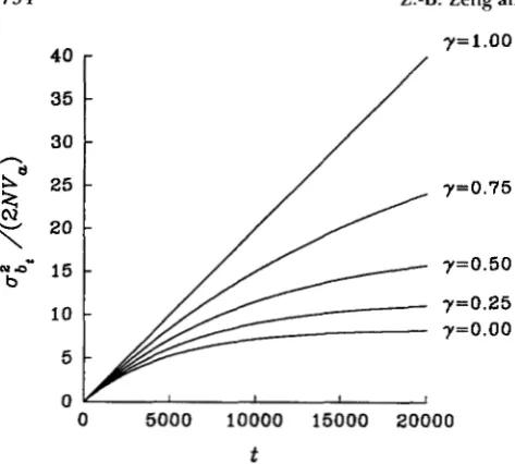
FIGURE 2.-Changes of d,/(2Wa) over time t from initially fixed populations for different values of y with N = 500 and u =

which agrees with the result of CHAKRABORTY and

NEI (1982) and LYNCH and HILL (1 986).

When we consider the randomly fixed founder

population (ie., c:,, = 0 and A = 0),

.zl

= (1

-

Sdt)a?*

-

2 ( P

-

Xf)ai* (23)

Figure 2 shows this ai,/(2NV,) for different values

with N = 500 and u = Expressed as a ratio over

2NV,, the variance with = 1 is always larger. For

a long time the parameter has little effect on

azt/(2NV,). Asymptotically, ai, converges to the

equilibrium at the rate of 1

-

CP E 2u(l

-

r),

and it

generally takes on the order of l/[u(l

-

r)]

genera-

tions to reach the equilibrium.

DISCUSSION

In this paper we proposed a mutation model called the regression mutation model which takes the random walk model and the house-of-cards model as two extremes. Though it tends to be more general than the extremes, the model is not a general mutation model. There could be numerous other ways to spec- ify the spectrum of effects of alleles and the mutation rates among them. However, the model does appear to be rather flexible and yet mathematically tractable. T h e basic features of the model are: (i) that the model

links the extremes by a structure parameter y and

offers a way to bridge the gap; (ii) that it imposes a

bound on the amount of overall availability of genetic

variation (like the house-of-cards model), and at the same time restricts the effect of a single step mutation (like the random walk model); and (iii) that mutation

will have a directional effect on the population mean

whenever it is away from the equilibrium point and

the effect is proportional to the deviation of the mean from the equilibrium point. These properties of the model appear to be desirable and realistic.

It should be pointed out here that the (strong)

house-of-cards mutation model proposed by KINCMAN

(1977, 1978) and discussed in this paper is quite

different from the (weak) house-of-cards mutation

model analyzed by TURELLI (1 984, 1986). In his analy-

sis of maintenance of genetic variance under the balance between mutation and stabilizing selection, TUR-

ELLI assumed that while the distribution of mutant effects is independent of the ancestral allele, it some- how depends on the population mean in such a way that there is no directional effect of mutation on the population mean, that is x ’ =

X

+

[ (TURELLI, 1986,

p. 616) where 35 denotes the average effect of alleles

segregating at the locus. It is not clear how the population mean provides a feedback to new mutations.

TURELLI proposed this version of the house-of-cards

model simply as an approximation to the random walk

model when the variance of mutant effects is signifi-

cantly larger than the existing genetic variance in the population.

T h e observation that the parameter y has little

effect on the ratios, kl/(2NV,) and az1/(2NV,), for quite some time, implies that practically the estimation

of the parameter V , or V, is little affected by mutation models because estimation of V, or V, is usually based

on the short-term accumulation of the genetic vari-

ances within and between populations (LYNCH 1988). However, in the long run, the genetic variances, particularly the genetic variance between populations, do depend on mutation models and can differ substan-

tially for different y. This can cause problems for

some statistical methods which rely on d , for testing

alternative hypotheses during macroevolution.

TURELLI, GILLESPIE and LANDE (1 988) proposed a

statistical method for testing for selection on quantitative characters during macroevolution. T h e idea is

that under the null hypothesis of neutrality, the mean,

it, of a quantitative character at generation t in a

population can be assumed to be approximately nor- mally distributed with mean i o and variance d l , i.e.,

z t

-

/Y [ i o ,

d J

(if the initial state of the population is assumed to be at the origin, or otherwise when y

<

1, the expected value of it is not necessarily i o and can be slightly

different from io, depending on the initial state of the

population as indicated by Equation

7).

If the ob-

served change of mean, z =

I

it

-

i o

I,

is tested to be

statistically too large or too small to be explained

solely by genetic drift, selection is indicated. Specifi- cally, for a test with 95% confidence, if

I

a b ,

I

41 >

2.24 (24)

(7)

explained by drift and thus directional selection may be indicated, and if

l i l

<

0.03

it is implied that evolution has been too slow to

be explained by drift and thus stabilizing selection

may be indicated, since P(I z/Ub,I

>

2.24) E 0.025 and

However, they used specifically the random walk mutation model as a null hypothesis when testing for selection. Under this model

P(J z / u ~ ,

I

<

0.03) E 0.025.

u;, = 2tVm

if the initial genetic variance within populations is at

mutation-drift equilibrium (ie., u&, = 2NVm). They

argued that even when the initial genetic variance

within populations is not at equilibrium, C T ~ , will be close to 2tVm for macroevolution. Thus for the test, they suggested to use

and

for Equations 24 and 25, where u2 is the phenotypic

variance of the character. If the bound, V,*(L)/u2 or Vt(U)/u2, is larger or smaller than typical estimates of

V,,,/u2, selection is indicated. [Note that TURELLI, GIL-

LESPIE and LANDE (1988) have emphasized that their test is just a qualitative test, not a rigorous statistical

test as the sampling distributions of estimates of pa-

rameters such as Vm are not considered.]

Obviously, this is a test under the random walk

mutation model, not a test under neutrality in general.

It is important to note that the random walk mutation

model is a mutation model, but not the only mutation

model. We showed before (COCKERHAM and TACHIDA

1987) and in this paper that depends on the mu-

tation model or the parameter y. For different values

of y, ui, can be markedly different when the time scale

is large, which is the case for testing during macro-

evolution. Although the true value of y is unknown,

it is reasonable to assume that y

<

1 . For example, if the initial populations are at the mutation-drift equilibrium (ie., u&, = u:, and A = O), for t = 5 X lo5 and

N = l o 6 [the parameter values used in one of the

examples in TURELLI, GILLESPIE and LANDE (1 988)],

0) = 3.96 for u = IO+; and ab,(-/ 2 = I)/u;,(y = 0.5) =

79.28 and ui,(y = l)/u?,(y = 0) = 205.01 for u = This illustrates that when tu

>

1 the ratio will increase

dramatically. As a matter of fact, when y = 1, uf +

GO as t + 03. This is the problem of the random walk

Ub,(Y 2 = l)/Ub,(y 2 = 0.5) = 2.86 and UEt (7 I)/u?,(y =

mutation model. Our analysis warns that the random walk mutation model (and also Turelli’s version of the house-of-cards model as it is consistent with the random walk model in this respect) should not be interpreted as a null hypothesis of neutrality for testing against alternative hypotheses of selection during ma-

croevolution. When t is large, using 2tVm as ui, will

allocate too much variation for z under the neutrality,

and, as a consequence, will decrease the probability of detecting directional selection and increase the probability of false detection for stabilizing selection.

We thank reviewers for useful comments, particularly for the clarification of the difference between the “strong” and “weak” house-of-cards mutation models. This investigation was supported in part by a National Institutes of Health Grant GM45344.

LITERATURE CITED

CHAKRABORTY, R., and M. NEI, 1982 Genetic differentiation of quantitative characters between populations or species. I . Mu- tation and random genetic drift. Genet. Res. 3 9 303-314.

CLAYTON, G. A., and A. ROBERTSON, 1955 Mutation and quantitative variation. Am. Nat. 89: 151-158.

COCKERHAM, C. C., and H. TACHIDA, 1987 Evolution and maintenance of quantitative genetic variation by mutations. Proc. Natl. Acad. Sci. USA 8 4 6205-6209.

CROW, J. F., and M. KIMURA, 1964 The theory of genetic loads. Proc. XI Int. Congr. Genet., pp. 495-505.

GREGORY, W. C., 1965 Mutation frequency, magnitude of change, and the probability of improvement in adaptation. Radiat. Bot. 5: (Suppl.) 429-441.

HILL, W. G., 1982 Predictions of response to artificial selection from new mutations. Genet. Res. 4 0 255-278.

KARLIN, S., and H. M. TAYLOR, 198 1 A Second Course in Stochastic Processes. Academic Press, New York.

KEIGHTLEY, P. D., and W. G. HILL, 1990 Variation maintained in quantitative traits with mutation-selection balance: pleio- tropic side-effects in fitness traits. Proc. R. SOC. Lond. B 242:

KIMURA, M., 1965 A stochastic model concerning the maintenance of genetic variability in quantitative characters. Proc. Natl. Acad. Sci. USA 5 4 731-736.

KINGMAN, J. F. C., 1977 On the properties of bilinear models for the balance between genetic mutation and selection. Proc. Cam. Philos. SOC. 81: 443-453.

KINCMAN, J. F. C., 1978 A simple model for the balance between selection and mutation. J. Appl. Prob. 15: 1-12.

LANDE, R., 1975 The maintenance of genetic variability by mutation in a polygenic character with linked loci. Genet. Res. 26: 221-235.

LI, W.-H., 1977 Maintenance of genetic variability under mutation and selection pressures in a finite population. Proc. Natl. Acad. Sci. USA 74: 2509-2513.

LYNCH, M., 1988 The rate of polygenic mutation. Genet. Res.

51: 137-148.

LYNCH, M., and W. G. HILL, 1986 Phenotypic evolution by neutral mutation. Evolution 40: 915-935.

MACKAY, T. F. C., R. F. LYMAN and M. S. JACKSON, 1992 Effects of P element inserts on quantitative traits in Drosophila mela- nogaster. Genetics 1 3 0 315-332.

MUKAI, T., 1964 The genetic structure of natural populations of

Drosophila melanogaster. I. Spontaneous mutation rates of polygenes controlling viability. Genetics 50: 1-19.

MUKAI, .T., S. I. CHIGUSA, L. E. METTLER and J. F. CROW,

1972 Mutation rate and dominance of genes affecting viabil-

(8)

ity in Drosophila melanogaster. Genetics 72: 335-355.

OKA, H. I . , J. HAYASHI and I. SHIOJIRI, 1958 Induced mutations of polygenes for quantitative characters in rice. J. Hered. 49:

OHTA, T., and H . TACHIDA, 1990 Theoretical study of near neutrality. 1. Heterozygosity and rate of mutant substitution. Genetics 1 2 6 219-229.

TURELLI, M., 1984 Heritable genetic variation via mutation-selection balance: Lerch’s zeta meets the abdominal bristle. Theor. Popul. Biol. 25: 138-193.

TURELLI, M., 1986 Gaussian versus non-Gaussian genetic analysis of polygenic mutation-selection balance, pp. 607-628 in Evo- lutionary Processes and Theory, edited by S. KARLIN and E. NEVO. Academic Press, New York.

11-14.

TURELLI, M . , J. H. GILLESPIE and R. LANDE, 1988 Rate tests for selection on quantitative characters during macroevolution and microevolution. Evolution 42: 1085-1089.

WATTERSON, G. A., 1977 Heterosis or neutrality? Genetics 85:

789-8 14.

WRIGHT, S., 1948 Genetics of populations, pp. 1 1 1-1 15 in Ency- clopaedia Britannica, Ed. 14, revised, Vol. 10. Encyclopaedia Britannica, Chicago.

WRIGHT, S., 1969 Evolution and the Genetics of Populations, Vol. 2. The Theory of Gene Frequencies. University of Chicago Press, Chicago.

ZENG, Z.-B., H. TACHIDA and C. C. COCKERHAM, 1989 Effects of mutation on selection limits in finite populations with multiple alleles. Genetics 122: 977-984.