AMP: a new time frequency feature extraction method for intermittent time series data

AMP: a new time-frequency feature extraction method for

intermittent time-series data

Duncan S. Barrack

Research Institute University of Nottingham

NG7 2TU, UK

duncan.barrack

@nottingham.ac.uk

James Goudling

Research Institute University of Nottingham

NG7 2TU, UK

james.goulding

@nottingham.ac.uk

Keith Hopcraft

Sciences University of Nottingham

NG7 2RD, UK

keith.hopcraft

@nottingham.ac.uk

Simon Preston

School of Mathematical Sciences University of Nottingham

NG7 2RD, UK

simon.preston

@nottingham.ac.uk

Gavin Smith

Research Institute University of Nottingham

NG7 2TU, UK

gavin.smith

@nottingham.ac.uk

ABSTRACT

The characterisation of time-series data via their most salient features is extremely important in a range of machine learn-ing task, not least of all with regards to classification and clustering. While there exist many feature extraction tech-niques suitable for non-intermittent time-series data, these approaches are not always appropriate forintermittent time-series data, where intermittency is characterized by constant values for large periods of time punctuated by sharp and transient increases or decreases in value.

Motivated by this, we presentaggregation, mode

decompo-sition and projection (AMP) a feature extraction technique

particularly suited to intermittent time-series data which contain time-frequency patterns. For our method all in-dividual time-series within a set are combined to form a non-intermittentaggregate. This is decomposed into a set of components which represent the intrinsic time-frequency sig-nals within the data set. Individual time-series can then be fit to these components to obtain a set of numerical features that represent their intrinsic time-frequency patterns. To demonstrate the effectiveness of AMP, we evaluate against the real word task of clustering intermittent time-series data. Using synthetically generated data we show that a cluster-ing approach which uses the features derived from AMP sig-nificantly outperforms traditional clustering methods. Our technique is further exemplified on a real world data set where AMP can be used to discover groupings of individu-als which correspond to real world sub-populations.

.

MiLeTS workshop in conjunction with KDD’ 15 August 10-13 2015, Sydney, Australia

Categories and Subject Descriptors

G.3 [Probability and Statistics]: time-series analysis

Keywords

time-series, feature extraction, intermittence

1.

INTRODUCTION

Extracting numerical features from time-series data is de-sirable for a number of reasons including revealing human interpretable characteristics of the data [43], data compres-sion [10] as well as clustering and classification [11, 20, 41]. It is often useful to divide the different feature extraction approaches into frequency domain and time domain based methods. Frequency domain extraction techniques include the discrete Fourier transform [39, 40] and wavelet trans-form [27]. Examples of time domain techniques are model based approaches [22] and more recently shapelets [45, 44].

Of particular interest to this paper are intermittent time-series data, such as that derived from human behavioural (inter-) actions, e.g. communications and retail transaction logs. Data of this type contains oscillatory time-frequency patterns corresponding to human behavioural patterns such as the 24 hour circadian rhythm, or 7 day working

week/weekend. It is also characterised by short periods of high activity followed by long periods of inactivity (inter-mittence) [1, 14, 16, 38]. Such characteristics mean that intermittent time-series feature sharp transitions in the de-pendent variable. When frequency based feature extraction techniques underpinned by the Fourier or wavelet transforms are applied, the transforms produceringing artefacts (a well known example in Fourier analysis is the Gibbs phenomena [12]) which results in spurious signals being produced in the spectra. These rogue signals make it extremely difficult to determine what the genuine frequency patterns in the data are. Furthermore, such signals are extremely damaging to clustering and classification techniques which use frequency or time-frequency features as inputs.

Another feature of intermittency is that it results in time-series that take a single, constant value for very large por-tions of the time domain. This phenomena severely de-grades the effectiveness of using time domain based extrac-tion methods for machine learning tasks. We will demon-strate not only the impact intermittent data has on tra-ditional extraction methods (showing that the more

mittent the data, the greater the deleterious impact of this effect) but go on to present a new solution to this issue.

The paper is structured as follows. In section 2 we demon-strate the issue of using traditional feature extraction tech-niques on intermittent data with a focus on the use of derived features for clustering. After discussing related work in Sec-tion 3 we introduce our ameliorative strategy in the form of Aggregation, mode decomposition and projection (AMP) in Section 4. We show in Section 5 that when features derived from AMP are used for clustering synthetically generated intermittent time-series data, results are significantly better than those which use traditional time-series clustering tech-niques. In this section, we also demonstrate that AMP gives promising results when applied a real communications data set. We conclude with a discussion in Section 6.

2.

BACKGROUND

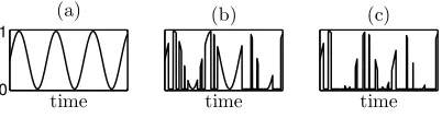
Although the concept of intermittence has received some ex-amination across various fields [8, 19] no accepted definition for the term currently exists. Consequently, in this work, we introduce our own expression which can be used to quantify intermittence in time-series. Before this is formally defined, to explain our rationale behind it we refer the reader to plots of three time different time-series in Figure 1, all with the same frequency pattern. Clearly time-series (a) is non-intermittent, with (b) being somewhat intermittent and (c) extremely intermittent - it takes a value of zero for large portions of the time domain, and consequently its frequency pattern is much harder to identify.

These observations leads us to construct a practical in-termittence measure based on the total proportion of the time domain that a time-series takes its most frequent value. In particular, if we regard a discrete time-series as a vector

x= (x1, x2, . . . , xn) of real valued elements sampled at equal

spaces in time as a realisation of a random process, then we define a measure of its intermittence by

φ(x) =P(xi=M(x)), (1)

whereM(x) is the mode, or most common value, in vector

xandP(xi=M(x)) is the empirical probability, or relative

frequency, that a randomly selected elementxiofxhas this

value. As a time-series becomes increasing intermittentφ will tend to 1. With this definition, time-series (a) in Figure 1 has a value for φ of 0.0001 reflecting the fact it is not intermittent. The intermittence measure of time-series (c) (0.7675) is higher than time-series (b) (0.4860) reflecting our observation that (c) is more intermittent than (b).

0 1

time (a)

time (b)

time (c)

Figure 1: Three example time-series illustrating the distinctions between a non-intermittent times series (a), partially intermittent time-series (b) and an extremely intermittent time-series (c).

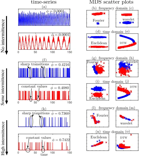
To illustrate the negative impact that intermittence has on the pertinence of features extracted using traditional techniques, let us first consider two distinct sets of non-intermittent time-series. We investigate what affect

increas-ing intermittence has on clusterincreas-ing results which use features obtained via the Fourier and wavelet transforms as well as clustering approaches which use the Euclidean and dynamic time warping (DTW) distance between individual time se-ries. The first set of time-series data is composed of 100 re-alisations of analmost periodically-drivenstochastic process [3] (see Section 5.1.1 for full details of this procedure), with period ranging linearly from 2 at the beginning of the simu-lation to 4 at the end (time-series from this set are depicted diagrammatically in blue). The second set also contains 100 time-series generated from an identical process, except for a period which ranges linearly from 8 to 16 (depicted di-agrammatically in red). Two examples from each set are illustrated in Figure 2a. Each of the time-series is plotted using the values for the first two dimensions obtained from classical multi-dimensional scaling (MDS) [5] of every coef-ficient value of each term in their direct discrete Fourier and wavelet decompositions (see Section 5.1 for full details of this procedure) in Figures 2b and 2c respectively. Additionally MDS results are shown where the Euclidean distance and DTW distance are used as the similarity measure between time series (Figures 2d and 2e respectively). Clearly, in this instance, a clustering approach based on any of these tech-niques is sufficient to discriminate the time-series from the two groups.

Next we consider what effect time-series with a greater value ofφ(and hence higher intermittence) has upon cluster-ing. These have the same time-frequency patterns as the cor-responding time-series in Figure 2a but are more intermit-tent. Examples are presented in Figure 2f and illustrate the sharp transitions and long periods for which the time-series take a constant value (some examples marked in the figure) that begin to occur in the data. Although it is still possible to discriminate the time-series in the MDS plots (Figures 2g-j), the sharp transitions in the data introduce ringing artefacts in the frequency based decompositions which re-sults in less well separated clusters (compare Figure 2g with 2b and Figure 2h with 2c). Furthermore, the large periods of constant values act to degrade the discriminative power of Euclidean and DTW based methods (compare Figure 2i with 2d and Figure 2j with 2e).

By the time we have increased intermittency further still to generate sets of 100 highly intermittent time-series (Fig-ure 2k) the negative impact of intermittency on clustering is severe and neither frequency domain based, Euclidean or DTW based methods can be used to separate the data (see Figure 2l-o).

3.

RELATED WORK

Numerous techniques for non-intermittent time-series fea-ture extraction, both time and frequency domain based, have been proposed. The most prevalent use of these within the machine learning community is to obtain numerical fea-tures for use as inputs for clustering and classification algo-rithms.

clas-time-series MDS scatter plots

No intermittence

(a)

0 50 100 150

φ= 0.0001

φ= 0.0001

wavelet

Euclidean DTW

time domain frequency domain

Fourier

(b) (c)

(d) (e)

Some intermittence

(f)

0 50 100 150

constant values _{φ= 0} .4080 sharp transitionsφ= 0.4216

frequency domain Fourier

time domain

Euclidean

DTW

(g) (h)

(i) (j)

wavelet

High intermittence

(k)

time

0 50 100 150

sharp transitionsφ= 0.7360

φ= 0.7422

constant values

frequency domain

time domain

DTW Euclidean

Fourier

wavelet

(l) (m)

(n) (o)

Figure 2: The impact of intermittency on cluster analy-sis. Plot (a) shows two non-intermittent time-series from a set of 200 which were generated via an almost peri-odically driven stochastic process, with periods ranging linearly from 2 to 4 for one half the set (blue) and 8 to 16 for the other half (red). Each time-series in the set of 200 is plotted using the values for the first two dimen-sions obtained from classical MDS of every coefficient value of the terms in their direct discrete Fourier (plot (b)) and wavelet decomposition (plot (c)) as well as of the Euclidean (plot (d)) and DTW (plot (e)) distance matrices. Plot (f ) shows time-series with increased in-termittency but with the same time-frequency pattern as in (a). The corresponding MDS plots are shown in plots (g-j). Finally, plot (k) shows highly intermittent time-series with associated MDS scatter plots in (l-o) il-lustrating the collapse in efficacy of cluster analysis. The value for the intermittenceφ(equation (1)) for the time-series are given in the figure insets.

sification [44] and unsupervised learning [45] with promising results. Model based approaches, where time-series data is fitted to a statistical model are also common. For example the linear predictive coding cepstrum coefficients obtained from fitting data to the autoregressive integrated moving average model have been used for clustering [15]. Although not strictly based on a feature extraction technique, an ef-fective approach with regards to time series learning is to use the raw, un-transformed time series data itself. It has been known for some time that using the Euclidean dis-tance as a similarity measure between time-series data can lead to extremely good clustering results [18]. Elastic mea-sures including DTW and edit distance, where the temporal alignment of data points isn’t respected, are also popular. An empirical study conducted on the data contained within the UCR time-series data mining archive [17] where the per-formance of numerous static and elastic measures on clas-sification was investigated suggested that DTW distance is the best measure [7].

Frequency domain based approaches are most commonly underpinned by the discrete Fourier or wavelet transforma-tion of the data. For example Vlachos et al used periodic features obtained partly via the direct Fourier decomposi-tion for clustering of MSN query log and electrocardiogra-phy time-series data [39]. Features derived from wavelet representations have also been used to cluster synthetic and electrical signals [27].

These works show that time domain and frequency do-main based features and distance measures can be extremely effective inputs to classification and clustering algorithms when time-series are non-intermittent. However, we not aware of any work which investigates how these approaches stand up againstintermittentdata or present feature extrac-tion approaches designed specifically for data of this type.

4.

AGGREGATION, MODE

DECOMPOSI-TION AND PROJECDECOMPOSI-TION (AMP)

Aggregate time-series generation. Given a set of m discrete time-seriesX={x1,x2, . . . ,xm}, where each

time-series xi = (xi1, xi2,· · ·xin) is represented by a vector of

length n with real valued elements, an aggregate is con-structed as follows

a=

m

X

i=1

xi. (2)

Under the assumption that each time-seriesiis a realisa-tion of a stochastic process with a positive probability that it will take a value other than the modal value, asm→ ∞, equation (2) will yield annon-intermittentaggregate. There is evidence to support the notion that much data can be re-garded as realisations of stochastic processes with a positive probability that an event will take place at any time. For ex-ample the times at which emails are sent has been modelled with a cascading non-homogeneous Poisson process with a positive rate function [25]. This model led to results with characteristics which were consistent with the characteristics of empirical data.

Time-frequency feature learning.Using a signal decom-position technique (e.g. Fourier or wavelet decomdecom-position)

ais decomposed intolcomponents

a=

l

X

j=1

bj, (3)

where each vectorbj = (bj1, bj2,· · ·, bjn) corresponds to a

different time-frequency component. To ensure that (3) does not include a constant term corresponding to the mean of the signal and only includes components corresponding to time-frequency patterns,ais mean centred (also know as ‘average centring’) prior to its decomposition. Series (3) is ordered in descending order of the total energy of each component

signal, i.e.

n

P

k=1

| b1k |2≥ n

P

k=1

| b2k |2≥ · · · ≥ n

P

k=1

| blk |2.

We discard time-frequency components that are not, or only minimally, expressed in the aggregate (these correspond to signals with the lowest energies) as such terms are often an artifact of noise in the data or the decomposition process itself. This is achieved by selecting the firstpterms of (3) (wherep≤l)

such that

p

P

j=1

n

P

k=1

|bjk|2

!

. n

P

k=1

|ak|2≥Et,

whereEt ∈[0,1] represents a selected threshold. This

pro-cedure ensures that only the components which correspond to the most salient time-frequency patterns of the aggregate are selected. Otherwise, the inclusion of terms correspond-ing to low energy time-frequency patterns in the subsequent projection step of AMP will result in the fitting of intermit-tent time-series to these unimportant patterns. In this work we setEt= 0.9, as we find such a value is sufficient to omit

low energy signals.

Next, each retained component of (3) is normalised (i.e. ˆ

bj=bj/|bj|). This step is key as it ensures that, during

the next step of our method, where each individual time-series is projected onto a set of basis vectors made up of the retained components, each basis vector will have equal weight. This ensures that basis vectors corresponding to components with extreme amplitudes will not skew results

in the projection step.

Basis vector projection. The final step in our method is to obtain a set of numerical features for each time-seriesxi

which indicate how much each time-frequency feature learnt from the aggregate is present in them. This is achieved by projecting eachxion to the set of normalised basis vectors.

In particular we seek the linear combination of basis vectors which is closest in the least-squares sense to the original observation, i.e. we minimise

||xiT−BbciT|| (4)

where then×pmatrixBb = (ˆbT1,bˆT2, . . . ,bˆTp) is comprised

of normalised basis vectors learnt from the aggregate. ci=

(ci1, ci2, . . . , cip) is a vector of fitted coefficients which form

the feature vector. The value of element cij indicates the

degree to which the time-frequency signal corresponding to normalised basis vectorj is expressed in time-seriesi.

Fitting allmtime-series to the set basis of vectors, as de-scribed above, yields the set of features{c1,c2,c3,. . . ,cm}.

This feature set therefore represents the extent to which an individual time-series expresses the time-frequency patterns present within the overall population. Clustering on this set will result in the grouping together of time-series with simi-lar time-frequency patterns and the clustering into different groups of those which exhibit different time-frequency pat-terns.

Choice of decomposition method for the aggregate time-series. We consider four methods for the decompo-sition of the aggregatea, which were selected based on the high prevalence in which they appear in the signal processing literature. These are described below.

Discrete Fourier decomposition. Using the discrete Fourier transform (DFT) [29] the aggregate is decomposed into a Fourier series. We set the number of Fourier components l= 1022. This ensures that the Fourier series approximates the aggregate extremely well for all data considered in this paper whilst, at the same time, being relatively computa-tionally inexpensive to obtain. We refer to the variant of AMP which uses Fourier decomposition for the aggregate as discrete Fourier transform AMP (DFT-AMP).

Discrete wavelet decomposition. This decomposition procedure takes a wavelet function and decomposes a time-series in terms of a set of scaled (stretched and compressed) and translated versions of this function [35]. Because of it’s prevalence of use within the scientific literature we use the Haar wavelet [24] for the mother wavelet. For consistency with DFT-AMP we ensure that the discrete wavelet trans-form produces 1022 components. This approach as discrete wavelet transform AMP (DWT-AMP).

AMP (DWPT-AMP).

Empirical Mode Decomposition.In contrast to Fourier and wavelet decomposition, empirical mode decomposition (EMD) [13] makes noa priori assumptions about the com-position of the time-series signal and as such is completely non-parametric. The method proceeds by calculating the envelope of the signal via spline interpolation of its max-ima and minmax-ima. The mean of this envelope corresponds to the intrinsic mode of the signal with the highest frequency and it is designated the firstintrinsic mode function(IMF). The first IMF is then removed from the signal and lower frequency IMFs are found by iteratively applying the mean envelope calculation step of the method. The number of IMFs produced is not fixed and depends on the number of intrinsic modes of the data. This variant of AMP is referred to as empirical mode decomposition AMP (EMD-AMP).

5.

EMPIRICAL EVALUATION

One of the most common reasons that researchers extract features from time-series is to serve as inputs for machine learning algorithms. Therefore, to assess the performance of AMP, we chose the real-world application of time series clus-tering. First we perform an evaluation of the effectiveness of DFT-AMP, DWT-AMP, DWPT-AMP and EMD-AMP us-ing synthetic data (in order that we have a ground to truth to assess against), showing that it outperforms traditional frequency domain and time domain based clustering tech-niques. We also show that across all variants, EMD-AMP is the most effective in partitioning data into groups with similar time-frequency patterns. With this demonstrated, EMD-AMP is then applied to a real world data set made up of the phone call logs of Massachusetts Institute of Technol-ogy (MIT) faculty and students [9]. The population of MIT individuals is clustered according to the IMFs they most ex-press with scatter plots revealing two distinct groupings that correspond to different departments in which the staff and students work.

5.1

Synthetic data

Each of our experiments involves two distinct groups of la-belled synthetic time-series. Each set includes a family of re-alizations generated by mixing two sinusoidal time-frequency patterns, with each set containing a distinct mix. Labels are removed, and the performance of all AMP variants is then evaluated by 1. extracting the time-frequency features ob-tained by each variant; 2. using these as inputs for cluster analysis; and 3. determining the extent to which the origi-nal set labels have been recovered. Clustering performance is compared to using traditional time-frequency feature extrac-tion methods and time domain based clustering approaches. The traditional methods considered for comparison are:

Fourier power clustering (Four. pow.). Here each time-seriesxiis decomposed into a Fourier series using the

DFT. The power of the components at each frequency is used as a feature for clustering. For consistency with the DFT-AMP approach, 1022 Fourier components are used.

Wavelet coefficient clustering (wav. coef.). Each time-series is decomposed via the DWT using the Haar wavelet and the coefficient values for each wavelet term are used as features for clustering. Again, each time-series is decom-posed into 1022 basis vectors.

Euclidean distance clustering (Euc.). Because of its simplicity and the fact such an approach can give excellent results [18], we consider a clustering approach based on the Euclidean distances between time-series.

Dynamic time warping distance clustering (DTW)

As evidence suggests that DTW distance is the most effec-tive distance measure for classification tasks [7] we investi-gate the performance of DTW distance between time-series on the clustering experiments using the standard DTW al-gorithm [2].

Four. pow., wav. coef., Euc. and DTW were used to obtain the results in Figure 2 in the introduction.

5.1.1

Data set generation

To produce our synthetic dataset we use a stochastic data generation model that underpins a model for the times at which emails are sent [25]. Such a model allows us to con-trol the the intermittency as well as the stationarity of the data, which is particularly useful given real world human activity data is often non-stationary [26, 37, 46]. We gener-ate three experimental datasets, the first in which all data is stationary (Syn1), the second in which non-stationary data is considered (Syn2), and the final set where noise is added to non-stationary data (Syn3). In order to investi-gate the impact of intermittency on the results we also vary the amount of intermittency the data exhibits.

To generate data sets of intermittent time-series with known time-frequency features (and hence known cluster member-ships) we, in the first instance, generate temporal point pro-cess data [6] with a prescribed generating function which controls the time-frequency patterns in the data. Synthetic time-series are then created by mapping the point process data to a continuous function by convolving the data with a kernel [36] as follows

xi(t) =

1 θi

ni X

k=1

K

t−tik

h

, (5)

where,tis time,tikis the kth point process event attributed

to time-seriesi,θithe total number of events generated and

K is the standard normal density function with bandwidth h. Function (5) is then sampled atnequally spaced points in time to obtain the discrete time-series xi. Thetik’s are

generated using a non-homogeneous Poisson process [32]. By utilising the rate function for the non-homogeneous Poisson process we can prescribe different time-frequency patterns in the synthetic time-series data. In each dataset, two equally sized groups of time-series are considered. Both express the same two time-frequency patterns but in different degrees. The data for each group is generated using the following rate functions which are sums of two almost periodic functions:

group 1:λ1(t) =ϕ

γsin2(_Tπt

1(t)) + (1−γ)sin

2

(_Tπt 2(t))

ifi≤m/2, (6)

group 2:λ2(t) =ϕ

(1−γ)sin2₍ πt

T1(t)) +γsin

2₍ πt

T2(t))

ifi > m/2, (7)

The amplitude coefficient,ϕ, effectively controls how

in-termittent the time-series is (smaller values lead to more

the same mix of time-frequency patterns and won’t be able to be distinguished. Otherwise the groups will express the same time-frequency patterns to different degrees, and as γ approaches zero will become increasingly distinct. The periodsT1andT2 of each sinusoidal function are defined as:

T1(t) =T10+α1t, T2(t) =T

0

2+α2t, (8)

where T10 and T

0

2 are constants. The coefficients α1 and

α2 act to allow non-stationary scenarios to be considered

where the period of oscillation of the rate functions (6) and (7) change with time.

These parameters allow us to produce three distinct ex-perimental datasets,Syn1, Syn2andSyn 3, against which we can evaluate performance. The datasets as described be-low:

Syn1: Stationary, No Noise

In this dataset,α1andα2 from equation (8) are both

set to 0 to ensure that the period of the rate functions of the non-homogeneous Poisson processes is fixed. T10

andT20 are set to 2 and 8 respectively.

Syn2: Non-Stationary, No Noise

As for Syn1, except α1 = 0.0078 and α2 = 0.0314

which ensures that the period of the rate functions are an increasing linear function of time. In particular, the period of rate function λ1(t) (resp. λ2(t)) from

equations (6) and (7) ranges from 2 (4) att= 0 to 4 (8) at t = 255. This means that the time-series are characterised by time-frequency patterns with period which increases with time.

Syn3: Non-Stationary, Noisy

As forSyn2, except noise is incorporated in one tenth of the time-series within the set. In particular,m/10 time-series were selected at random. Of the temporal events from which these time-series were formed, 50 are selected at random and an additional 41 events (equally distributed over a period of 0.02 time units) are introduced starting from the selected time point. This gives a total of 2050 additional events per time-series selected. These manifests themselves as ‘spikes’ in the time-series where the value of the dependent variable rises and falls extremely quickly.

5.1.2

Results

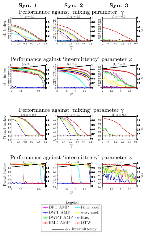
Results of the synthetic experiments are shown in Figure 3. The performance of the methods presented in this paper are measured firstly by the mean silhouette score [33] for all data points in a set against the true clustering in two dimensions (obtained via classical MDS where applicable). A score of 1 indicates maximal distance between the two true clusters (i.e. between the data points of groups 1 and 2), with 0 corresponding to maximal mixing between the clusters. The performance is also measured via the Rand index [31] between the true clustering and that obtained from the application ofk-means (k= 2) [23] to the full set of features outputted by each method. Here, 1 corresponds to perfect agreement between thek-means results and the true clustering. For each data set the effects of varying the mixing parameterγ and amplitude parameterϕ(equations (6) and (7)) are also considered.

The results illustrate that all AMP variants consistently outperform state of the art techniques (wav. coef., Four.

Syn. 1 Syn. 2 Syn. 3

Performance against ‘mixing parameter’γ

0 0.1 0.2 0.3 0.4 0.5

0 0.1 0.2 0.3 0.4 0.5 0.6 0.7 0.8 0.9

1 (a)ϕ= 0.3

0 0.2 0.4 0.6 0.8 1 0 0.2 0.4 0.6 0.8 1 0 0.2 0.4 0.6 0.8 1 0 0.2 0.4 0.6 0.8 1 0 0.2 0.4 0.6 0.8 1 0 0.2 0.4 0.6 0.8 1 0 0.2 0.4 0.6 0.8 1 0 0.2 0.4 0.6 0.8 1

0 0.1 0.2 0.3 0.4 0.5

0 0.1 0.2 0.3 0.4 0.5 0.6 0.7 0.8 0.9

1 b)ϕ= 0.3

0 0.2 0.4 0.6 0.8 1 0 0.2 0.4 0.6 0.8 1 0 0.2 0.4 0.6 0.8 1 0 0.2 0.4 0.6 0.8 1 0 0.2 0.4 0.6 0.8 1 0 0.2 0.4 0.6 0.8 1 0 0.2 0.4 0.6 0.8 1 0 0.2 0.4 0.6 0.8 1

0 0.1 0.2 0.3 0.4 0.5

0 0.1 0.2 0.3 0.4 0.5 0.6 0.7 0.8 0.9

1 c)ϕ= 0.3

0 0.2 0.4 0.6 0.8 1 0 0.2 0.4 0.6 0.8 1 0 0.2 0.4 0.6 0.8 1 0 0.2 0.4 0.6 0.8 1 0 0.2 0.4 0.6 0.8 1 0 0.2 0.4 0.6 0.8 1 0 0.2 0.4 0.6 0.8 1 0 0.2 0.4 0.6 0.8 1

Performance against ‘intermittency’ parameterϕ

0.5 1 1.5 2 0 0.1 0.2 0.3 0.4 0.5 0.6 0.7 0.8 0.9

1 (d)β= 0

0 0.2 0.4 0.6 0.8 1 0 0.2 0.4 0.6 0.8 1 0 0.2 0.4 0.6 0.8 1 0 0.2 0.4 0.6 0.8 1 0 0.2 0.4 0.6 0.8 1 0 0.2 0.4 0.6 0.8 1 0 0.2 0.4 0.6 0.8 1 0 0.2 0.4 0.6 0.8 1 0.5 1 1.5 2 0 0.1 0.2 0.3 0.4 0.5 0.6 0.7 0.8 0.9

1 (e)β= 0

0 0.2 0.4 0.6 0.8 1 0 0.2 0.4 0.6 0.8 1 0 0.2 0.4 0.6 0.8 1 0 0.2 0.4 0.6 0.8 1 0 0.2 0.4 0.6 0.8 1 0 0.2 0.4 0.6 0.8 1 0 0.2 0.4 0.6 0.8 1 0 0.2 0.4 0.6 0.8 1 0.5 1 1.5 2 0 0.1 0.2 0.3 0.4 0.5 0.6 0.7 0.8 0.9

1 (f)β= 0

0 0.2 0.4 0.6 0.8 1 0 0.2 0.4 0.6 0.8 1 0 0.2 0.4 0.6 0.8 1 0 0.2 0.4 0.6 0.8 1 0 0.2 0.4 0.6 0.8 1 0 0.2 0.4 0.6 0.8 1 0 0.2 0.4 0.6 0.8 1 0 0.2 0.4 0.6 0.8 1

Performance against ‘mixing’ parameterγ

0 0.1 0.2 0.3 0.4 0.5

0.4 0.5 0.6 0.7 0.8 0.9

1 (g)ϕ= 0.3

0 0.2 0.4 0.6 0.8 1 0 0.2 0.4 0.6 0.8 1 0 0.2 0.4 0.6 0.8 1 0 0.2 0.4 0.6 0.8 1 0 0.2 0.4 0.6 0.8 1 0 0.2 0.4 0.6 0.8 1 0 0.2 0.4 0.6 0.8 1 0 0.2 0.4 0.6 0.8 1

0 0.1 0.2 0.3 0.4 0.5

0.4 0.5 0.6 0.7 0.8 0.9

1 (h)ϕ= 0.3

0 0.2 0.4 0.6 0.8 1 0 0.2 0.4 0.6 0.8 1 0 0.2 0.4 0.6 0.8 1 0 0.2 0.4 0.6 0.8 1 0 0.2 0.4 0.6 0.8 1 0 0.2 0.4 0.6 0.8 1 0 0.2 0.4 0.6 0.8 1 0 0.2 0.4 0.6 0.8 1

0 0.1 0.2 0.3 0.4 0.5

0.4 0.5 0.6 0.7 0.8 0.9

1 (i)ϕ= 0.3

0 0.2 0.4 0.6 0.8 1 0 0.2 0.4 0.6 0.8 1 0 0.2 0.4 0.6 0.8 1 0 0.2 0.4 0.6 0.8 1 0 0.2 0.4 0.6 0.8 1 0 0.2 0.4 0.6 0.8 1 0 0.2 0.4 0.6 0.8 1 0 0.2 0.4 0.6 0.8 1

Performance against ‘intermittency’ parameterϕ

0.5 1 1.5 2 0.4 0.5 0.6 0.7 0.8 0.9

1 (j)β= 0

0 0.2 0.4 0.6 0.8 1 0 0.2 0.4 0.6 0.8 1 0 0.2 0.4 0.6 0.8 1 0 0.2 0.4 0.6 0.8 1 0 0.2 0.4 0.6 0.8 1 0 0.2 0.4 0.6 0.8 1 0 0.2 0.4 0.6 0.8 1 0 0.2 0.4 0.6 0.8 1 0.5 1 1.5 2 0.4 0.5 0.6 0.7 0.8 0.9

1 (k)β= 0

0 0.2 0.4 0.6 0.8 1 0 0.2 0.4 0.6 0.8 1 0 0.2 0.4 0.6 0.8 1 0 0.2 0.4 0.6 0.8 1 0 0.2 0.4 0.6 0.8 1 0 0.2 0.4 0.6 0.8 1 0 0.2 0.4 0.6 0.8 1 0 0.2 0.4 0.6 0.8 1 0.5 1 1.5 2 0.4 0.5 0.6 0.7 0.8 0.9

1 (l)β= 0

0 0.2 0.4 0.6 0.8 1 0 0.2 0.4 0.6 0.8 1 0 0.2 0.4 0.6 0.8 1 0 0.2 0.4 0.6 0.8 1 0 0.2 0.4 0.6 0.8 1 0 0.2 0.4 0.6 0.8 1 0 0.2 0.4 0.6 0.8 1 0 0.2 0.4 0.6 0.8 1

Figure 3: Plots (a)-(f ) show the mean silhouette index score for the two dimensional representations of the fea-ture values obtained using all methods detailed in Sec-tions 4 and 5. Scores are plotted as a function of the mix-ing parameter γ(a-c) and amplitude parameterϕ (d-f ). Note that intermittence increases asϕ decreases. Plots (g)-(l) show the Rand index scores obtained by compar-ing the results ofk-means clustering applied to the full set of coefficient scores for each method to the true clus-tering. The average intermittence scoreφ¯(equation (1)) for all time-series in a set is also shown in each plot (value given in the right axes). For each value of γand ϕ con-sidered, ten simulations were run and an average taken for the mean silhouette score, Rand index and mean in-termittence score. Parameter values for all simulations

are m= 4000, h= 0.05 and where given in Section 5.1.1

pow, Euc. and DTW) in every plot except for the DWT-AMP variant, the performance of which is comparable to wav. coef. and Four. pow. Of all variants, EMD-AMP is the best performer. This is particularly noticeable when the data sets are both non-stationary and contain noise (see plots (c,f,i,l). All frequency domain based methods outper-form the time domain based methods (Euc. and DTW). This latter results highlights that DTW and Euclidean dis-tance based methods are not suitable for the clustering of intermittent data. As expected, the performance of every method decreases as the mixing parameterγ increases and amplitude parameterϕ(which is inversely related to inter-mittence) decreases.

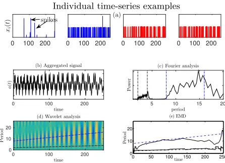
To aid our explanation as to why AMP appears to be per-forming so well in producing accurate time-frequency fea-tures for intermittent data and why, of all the variants, EMD-AMP produces the most accurate features, we con-sider a specific instance of Syn3, the non-stationary and noisy data set. We use the same parameter values for syn-thetic data generation as those used in Figure 3l and set γ = 0 (ensuring that the time-frequency patterns of both groups are as distinct as can be, with each group expressing completely different time-frequency patterns) . The period of oscillation of group 1 time-series ranges linearly from 2 at t= 0 to 4 att= 255 and group 2 data from 4 to 8.

A sample of individual time-series from each group, to-gether with the aggregate and spectrograms obtained from its decomposition are shown in Figure 4. Despite the in-termittent nature of the individual time-series, the aggre-gate is clearly non-intermittent (Figure 4b). Furthermore, the noise present in some time-series has been suppressed by the aggregation process. The non-intermittence of the aggregate time-series is one of the strengths of the AMP approach as it permits decompositions which do not con-tain spurious signals corresponding to ringing artefacts. In particular wavelet and EMD decompositions reveal only the two time-frequency patterns (one with period ranging from 2 to 4 and the other with period from 4 to 8) which are present within the data set (Figures 4d and 4e respectively). Because the aggregated signal is non-stationary with time varying frequency components, the Fourier spectrum picks up the range in frequencies of the underlying time-frequency patterns but gives no indication as towhendifferent frequen-cies are present in the aggregate (Figure 4c).

Scatter plots of the time-frequency features obtained using every AMP method considered in this work are shown in Figure 5. These have been symbolised based on whether the time-series are members of group 1 (blue symbols) or group 2 (red symbols). EMD-AMP (Figure 5d) clearly clusters the two groups according to the time-frequency patterns they most express. So do DFT-AMP (a) and DWPT-AMP (c), but not to the same extent. DWT-AMP (b) fails to cluster the data correctly in this instance.

The success of EMD-AMP is related to the fact that its basis vectors permit a more parsimonious model of the data’s underlying time-frequency patterns. Indeed for all cases con-sidered in this section, applying EMD to the aggregate pro-duces just two IMFs - each corresponding to one of the two intrinsic time-frequency patterns of the data. This is still true even when such patterns are non-stationary with time varying frequencies.

In contrast, Fourier basis vectors (with their fixed frequen-cies) are incapable of succinctly modelling the intrinsic

time-frequency patterns that exist in data with a time-frequency that varies over time. Similarly, the rigidity of the DWT means it produces wavelet vectors which individually only model an underlying time-frequency pattern for a small proportion of timeand for a small proportion of its frequency band. The basis vectors produced via the DWPT can only individually model either (i) a proportion of the frequency of an under-lying pattern over the whole time domain, (ii) all of the un-derlying patterns frequency band but only for a short period of time, or (iii) neither. This means that no single basis vec-tor obtained via the DFT, DWT or DWPT may individually capture the complete time-frequency patterns that underpin non-stationary data. Despite these weaknesses, these basis vectors are sufficiently similar to underlying time-frequency patterns within the data for DFT-AMP, DWT-AMP and DWPT-AMP to still yield reasonable results.

It is also notable that for stationary data (see the results in Figure 3 (a,d,g,j)) the performances of EMD-AMP, DFT-AMP and DWPT-DFT-AMP are almost identical. In this in-stance, this is due to each method decomposing the aggre-gate into two almost identical components: one correspond-ing to the intrinsic oscillation with fixed period 2 and the other to the oscillation with fixed period 4.

Individual time-series examples

0 100 200

xi

(

t

)

0 100 200 0 100 200 0 100 200

spikes (a)

time

0 100 200

a

(

t

)

(b) Aggregated signal

period

5 10 15 20

P

ow

er

(c) Fourier analysis

(d) Wavelet analysis

time

0 100 200

P

er

io

d

0 10 20

0 50 100 150 200 250

0 10 20

time

P

er

io

d

(e) EMD

Figure 4: The top plots shows four individual time-series, two from group 1 (blue lines) and two from group 2 (red lines) illustrating the intermittent nature of the data. The first of these was generated from data contain-ing noise which manifests itself as ‘spikes’ (some exam-ples marked) in the time-series. The plot also shows the aggregate (equation (2)) obtained by combining all 4000 intermittent time-series in the set. The non-intermittent aggregate permits wavelet and empirical model decom-positions which reveal the two underlying time-frequency patterns (indicated by blue and red broken lines in the

spectrum) of the data set. Note, the edge effects in

the EMD plot are artefacts resulting from the discrete Hilbert transform of the IMFs. The Fourier spectra is also shown and this picks up the range of the frequencies of the two time-frequency patterns (indicated by blue and red broken lines).

Matlab code used to produce the synthetic data and ob-tain the results in this section is available at

Dim. 1

D

im

.

2

(a) DFT AMP

Dim. 1

D

im

.

2

(b) DWT AMP

Dim. 1

D

im

.

2

(c) DWPT AMP

Dim. 1

D

im

.

2

(d) EMD AMP

Figure 5: Scatter plots indicating that EMD-AMP (d) and, to a lesser extent, DFT-AMP (a) and DWPT-AMP (c) can be used to cluster data according to the time-frequency pattens most expressed. Results obtained by plotting the coefficient values outputted by each method (after classical MDS to two dimensions where appropri-ate) for 200 randomly selected time-series (100 from each group 1 (blue symbols) and 100 from group 2 (red sym-bols)). The average value for intermittency over all time-series in the setφ¯ is 0.8697. Parameter values for syn-thetic data generation as for Figure 3l exceptϕ= 1.5.

5.2

MIT reality mining data set

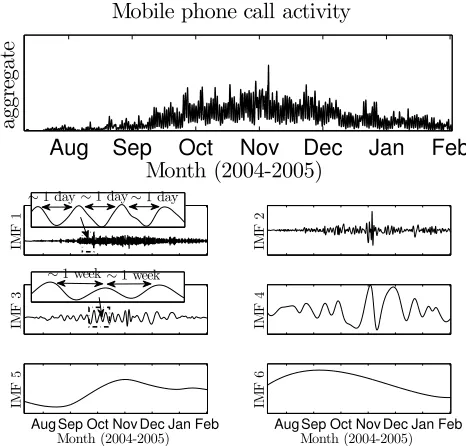
In order to provide evidence that AMP can be used to achieve meaningful results when applied to real world data we consider the MIT Reality Mining dataset. This set com-prises event data pertaining to the times and dates at which MIT staff and students made a total of 54 440 mobile phone calls over a period from mid 2004 until early 2005. The av-erage intermittency measure across the population is high ( ¯φ= 0.544) and thus the data set is an excellent candidate for the AMP method. While no ground truth exists for this data, we utilise additional co-variates within the data set as a qualitative proxy for a ground truth for a useful segmen-tation. In particular, we use participants’ affiliation (Media lab or Sloan business school, see [9] for details) as the proxy. Because of its excellent performance in the previous section, we choose to use the EMD-AMP variant.

5.2.1

Results

The aggregate and normalised IMFs of the MIT data are shown in Figure 6. Interestingly, many of the IMFs have a physical interpretation. The first IMF has a period of almost exactly a day. This is most likely generated by the natural 24-hour circadian rhythm which will cause individuals to make a large proportion of their phone calls during the day and early evening. IMF 3 has a period of one week and most likely corresponds to the propensity of study participants to make more phone calls during the working week than at weekends. IMF 6 peaks in September/October before falling again in December/January. It is likely that this function corresponds to the changes in activity between the Fall term (September to December/January) and the holiday periods

(over the summer and after Christmas) at MIT.

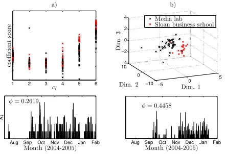
The extracted feature values for the 65 individuals who make the most phone calls are plotted in Figure 7, together with two clearly intermittent time-series of two randomly chosen individuals. The scatter plots have been symbolised based on whether the individuals were members of the re-ality mining group or the Sloan business school at MIT. In-terestingly, from the three dimensional representation (Fig-ure 7b) of the feat(Fig-ure values, with the exception of a hand-ful of individuals, the individuals from the two groups are separated from each other. Recall that the higher the fea-ture value, the more the corresponding IMF is expressed in that individual’s communications activity. From Figure 7a it can be seen that Sloan business school affiliates (red sym-bols) have, on average, larger coefficient values correspond-ing to IMFs 4-6 than the Media lab affiliates (black sym-bols). From this we can infer that the frequency patterns corresponding to IMFs 4-6 are expressed more strongly in the communication patterns of members of the Sloan busi-ness school.

Aug

Sep

Oct

Nov

Dec

Jan

Feb

ag

gr

eg

at

e

Mobile phone call activity

Month (2004-2005)

IM

F

1

IM

F

2

IM

F

3

IM

F

4

Aug Sep Oct Nov Dec Jan Feb

IM

F

5

Month (2004-2005)

Aug Sep Oct Nov Dec Jan Feb

IM

F

6

Month (2004-2005) ∼1 day∼1 day

∼1 day

∼1 week ∼1 week

Figure 6: Aggregate signal and decomposition obtained via EMD revealing six intrinsic time-frequency patters of the MIT communications data. IMF 1 has a period of 1 day and corresponds to the circadian cycle, while IMF 3 has a period of a week and corresponds to the seven day working week/weekend cycle.

6.

CONCLUSIONS AND FURTHER WORK

us-1 2 3 4 5 6

co

e

ffi

ci

en

t

sc

or

e

ci

a)

−5

0 5

−10 0 10 −4 −2 0 2 4

D

im

.

3

b)

Dim. 1 Dim. 2

Media lab Sloan business school

Aug Sep Oct Nov Dec Jan Feb

xi

Month (2004-2005)

φ= 0.2619

Aug Sep Oct Nov Dec Jan Feb

Month (2004-2005)

φ= 0.4458

Figure 7: Scatter plots indicating that Media lab and Sloan business school affiliates can be clustered accord-ing the the time-frequency patterns they most express. a) shows fitted coefficient values corresponding to each IMF. b) is a three dimensional representation of this data obtained via classical MDS. The bottom plots show the time-series of two study participants which are both clearly intermittent (intermittency measure valuesφare given in the plots).

ing Matlab on a PC utilising single 3.2 GHz processor). We note that even though our intermittence measure (equation (2)) may not capture the degree of intermittence of all types of intermittent data, AMP will still be effective in these sit-uations.

In terms of further work, it would be interesting to com-pare the performance of AMP clustering to techniques not considered in this paper such as a clustering approach un-derpinned by the Lomb-Scargle Periodogram [21] which was developed specifically for irregularly sampled data. Another time-domain based clustering method which we did not con-sider is the recently proposed shapelet based clustering ap-proach [45] where ‘local patterns’ in the data are exploited. However, as the values of intermittent times-series fluctu-ate only briefly from the the modal value, data rarely dis-plays meaningful local patterns and our intuition is that shapelet based clustering is not appropriate in this instance. A comparison with model based approaches such those un-derpinned by switching Kalman filters [28] would also be interesting.

The focus of this paper’s evaluation has been on using AMP derived features for clustering. However, AMP fea-tures are also suited to the classification task. There is huge scope to apply an AMP based clustering and/or classi-fication approach to many other types of intermittent time-series data and this would provide an interesting avenue for future work. For example, retail transaction data is char-acterised by the sporadic activity of customers who make a small number of purchases over a long period of time. The timings of these purchases will be dictated by time-frequency patterns corresponding to human behavioural pat-terns such as the 24 hour circadian rhythm, or 7 day work-ing week/weekend. Another example is the number of trips made by an individual on public transport. These are un-likely to total more than a handful per day, but the timings of these trips is likely to follow time-frequency patterns cor-responding to the traveller’s commuting behaviour or leisure

plans.

7.

ACKNOWLEDGEMENTS

This work was funded by EPSRC grant EP/G065802/1 -Horizon: Digital Economy Hub at the University of Notting-ham and EPSRC grant EP/L021080/1 - Neo-demographics: Opening Developing World Markets by Using Personal Data and Collaboration.

8.

REFERENCES

[1] A. Barab´asi. The origin of bursts and heavy tails in human dynamics.Nature, 435(7039):207–211, 2005. [2] D. J. Berndt and J. Clifford. Using dynamic time

warping to find patterns in time series. InProceedings

of KDD workshop, 1994.

[3] P. H. Bezandry and T. Diagana.Almost periodic

stochastic processes. Springer, 2011.

[4] R. R. Coifman and M. V. Wickerhauser.

Entropy-based algorithms for best basis selection.

IEEE Transactions on Information Theory,

38(2):713–718, 1992.

[5] T. F. Cox and M. A. Cox.Multidimensional scaling. CRC Press, 2010.

[6] D. Daley and D. Vere-Jones.An introduction to the theory of point processes: Volume II: general theory

and structure. Springer, 2007.

[7] H. Ding, G. Trajcevski, P. Scheuermann, X. Wang, and E. Keogh. Querying and mining of time series data: experimental comparison of representations and distance measures.Proceedings of the VLDB

Endowment, 1(2):1542–1552, 2008.

[8] M. Ding. Intermittency. In A. Scott, editor,

Encyclopedia of nonlinear science, pages 463–464.

Routledge, 2013.

[9] N. Eagle, A. Pentland, and D. Lazer. Inferring friendship network structure by using mobile phone data.Proceedings of the National Academy of Sciences

U.S.A., 106(36):15274–15278, 2009.

[10] T. Fu. A review on time series data mining.

Engineering Applications of Artificial Intelligence,

24(1):164–181, 2011.

[11] D. Garrett, D. A. Peterson, C. W. Anderson, and M. H. Thaut. Comparison of linear, nonlinear, and feature selection methods for EEG signal

classification.IEEE Transactions on Neural Systems

and Rehabilitation Engineering, 11(2):141–144, 2003.

[12] J. Gibbs. Fourier’s series.Nature, 59:606, 1899. [13] N. Huang et al.The empirical mode decomposition

and the hilbert spectrum for nonlinear and

non-stationary time series analysis.Proceedings of the

Royal Society A, 454(1971):903–995, 1998.

[14] H. Jo, M. Karsai, J. Kert´esz, and K. Kaski. Circadian pattern and burstiness in mobile phone

communication.New Journal of Physics, 14(1):013055, 2012.

[15] K. Kalpakis, D. Gada, and V. Puttagunta. Distance measures for effective clustering of ARIMA

time-series. InData Mining, 2001. ICDM 2001,

Proceedings IEEE International Conference on, pages

[16] M. Karsai, K. Kaski, A. Barab´asi, and J. Kert´esz. Universal features of correlated bursty behaviour.

Scientific reports, 2, 2012.

[17] E. Keogh and T. Folias. The UCR Time Series Data Mining Archive [http://www. cs. ucr. edu/∼

eamonn/time series data/]. Riverside CA.University of California-Computer Science & Engineering

Department, 2008.

[18] E. Keogh and S. Kasetty. On the need for time series data mining benchmarks: a survey and empirical demonstration.Data Mining and Knowledge

Discovery, 7(4):349–371, 2003.

[19] ¨O. Ki¸si. Neural networks and wavelet conjunction model for intermittent streamflow forecasting.Journal

of Hydrologic Engineering, 14(8):773–782, 2009.

[20] T. W. Liao. Clustering of time series data - a survey.

Pattern Recognition, 38(11):1857–1874, 2005.

[21] N. R. Lomb. Least-squares frequency analysis of unequally spaced data.Astrophysics and space science, 39(2):447–462, 1976.

[22] I. L. MacDonald and W. Zucchini.Hidden Markov

and other models for discrete-valued time series,

volume 110. CRC Press, 1997.

[23] J. MacQueen. Some methods for classification and analysis of multivariate observations. InProceedings of the fifth Berkeley symposium on mathematical

statistics and probability, volume 1, pages 281–297.

University of California Press, 1967.

[24] S. Mallat.A wavelet tour of signal processing. Academic press, 1999.

[25] R. Malmgren, D. Stouffer, A. Motter, and L. Amaral. A poissonian explanation for heavy tails in e-mail communication.Proceedings of the National Academy

of Sciences U.S.A., 105(47):18153–18158, 2008.

[26] R. D. Malmgren, D. B. Stouffer, A. S. Campanharo, and L. A. N. Amaral. On universality in human correspondence activity.Science, 325(5948):1696–1700, 2009.

[27] M. Misiti, Y. Misiti, G. Oppenheim, and J.-M. Poggi. Clustering signals using wavelets. InComputational and Ambient Intelligence, Lecture Notes in Computer

Science, volume 4507.

[28] K. P. Murphy. Switching kalman filters. Technical report, DEC/Compaq Cambridge Research Labs, 1998.

[29] A. V. Oppenheim, R. W. Schafer, J. R. Buck, et al.

Discrete-time signal processing, volume 2.

Prentice-Hall Englewood Cliffs, 1989.

[30] G. Oppenheim.Wavelets and Statistics, Lecture notes

in Statistics, volume 103. Springer Verlag, 1995.

[31] W. M. Rand. Objective criteria for the evaluation of clustering methods.Journal of the American

Statistical Association, 66(336):846–850, 1971.

[32] S. M. Ross.Introduction to probability models. Academic Press, 2006.

[33] P. Rousseeuw. Silhouettes: a graphical aid to the interpretation and validation of cluster analysis.

Journal of Computational and Applied Mathematics,

20:53–65, 1987.

[34] T. Schreiber and A. Schmitz. Classification of time series data with nonlinear similarity measures.

Physical review letters, 79(8):1475, 1997.

[35] Y. Sheng. Wavelet transform. In A. D. Poularikas, editor,The transforms and applications handbook,

second edition, Electrical engineering handbook.

Taylor & Francis, 2000.

[36] B. Silverman.Density estimation for statistics and

data analysis. Chapman & Hall, 1986.

[37] J. Stehl´e, A. Barrat, and G. Bianconi. Dynamical and bursty interactions in social networks.Physical review E, 81(3):035101, 2010.

[38] A. V´azquez, J. G. Oliveira, Z. Dezs¨o, K.-I. Goh, I. Kondor, and A. Barab´asi. Modeling bursts and heavy tails in human dynamics.Physical Review E, 73(3):036127, 2006.

[39] M. Vlachos, S. Y. Philip, and V. Castelli. On periodicity detection and structural periodic

similarity. InSIAM International Conference on Data

Mining, volume 5, pages 449–460. SIAM, 2005.

[40] M. Vlachos, S. Y. Philip, V. Castelli, and C. Meek. Structural periodic measures for time-series data.Data

Mining and Knowledge Discovery, 12(1):1–28, 2006.

[41] X. Wang, K. Smith, and R. Hyndman.

Characteristic-based clustering for time series data.

Data Mining and Knowledge Discovery, 13(3):335–364,

2006.

[42] A. Wolf, J. B. Swift, H. L. Swinney, and J. A.

Vastano. Determining lyapunov exponents from a time series.Physica D: Nonlinear Phenomena,

16(3):285–317, 1985.

[43] Z. Xing, J. Pei, S. Y. Philip, and K. Wang. Extracting interpretable features for early classification on time series. InSIAM International Conference on Data

Mining, volume 11, pages 247–258. SIAM, 2011.

[44] L. Ye and E. Keogh. Time series shapelets: a new primitive for data mining. InProceedings of the 15th ACM SIGKDD International Conference on

Knowledge Discovery and Data Mining, pages

947–956. ACM, 2009.

[45] J. Zakaria, A. Mueen, and E. Keogh. Clustering time series using unsupervised-shapelets. InIEEE

International Conference on Data Mining, 2012.

[46] K. Zhao, J. Stehl´e, G. Bianconi, and A. Barrat. Social network dynamics of face-to-face interactions.Physical