Dark matter halo properties of GAMA galaxy groups from 100 square degrees of KiDS weak lensing data

Dark matter halo properties of GAMA galaxy groups from 100 square

degrees of KiDS weak lensing data

M. Viola,

M. Cacciato,

M. Brouwer,

K. Kuijken,

H. Hoekstra,

P. Norberg,

A. S. G. Robotham,

E. van Uitert,

M. Alpaslan,

I. K. Baldry,

A. Choi,

J. T. A. de Jong,

S. P. Driver,

T. Erben,

A. Grado,

Alister W. Graham,

C. Heymans,

H. Hildebrandt,

A. M. Hopkins,

N. Irisarri,

B. Joachimi,

J. Loveday,

L. Miller,

R. Nakajima,

P. Schneider,

C. Sif´on

and G. Verdoes Kleijn

1_{Leiden Observatory, Leiden University, Niels Bohrweg 2, NL-2333 CA Leiden, the Netherlands} 2_{ICC, Department of Physics, Durham University, South Road, Durham DH1 3LE, UK}

3_{ICRAR, School of Physics, University of Western Australia, 35 Stirling Highway, Crawley, WA 6009, Australia} 4_{Department of Physics and Astronomy, University College London, Gower Street, London WC1E 6BT, UK} 5_{Argelander-Institut f¨ur Astronomie, Auf dem H¨ugel 71, D-53121 Bonn, Germany}

6_{NASA Ames Research Centre, N232, Moffett Field, Mountain View, CA 94035, USA}

7_{Astrophysics Research Institute, Liverpool John Moores University, IC2, Liverpool Science Park, 146 Brownlow Hill, Liverpool L3 5RF, UK} 8_{Scottish Universities Physics Alliance, Institute for Astronomy, University of Edinburgh, Royal Observatory, Blackford Hill, Edinburgh EH9 3HJ, UK} 9_{Scottish Universities’ Physics Alliance (SUPA), School of Physics and Astronomy, University of St Andrews, North Haugh, St Andrews, KY16 9SS, UK} 10_{INAF-Osservatorio Astronomico di Capodimonte, Via Moiariello 16, I-80131 Napoli, Italy}

11_{Centre for Astrophysics and Supercomputing, Swinburne University of Technology, Hawthorn, VIC 3122, Australia} 12_{Australian Astronomical Observatory, PO Box 915, North Ryde, NSW 1670, Australia}

13_{Astronomy Centre, University of Sussex, Falmer, Brighton BN1 9QH, UK} 14_{Department of Physics, Oxford University, Keble Road, Oxford OX1 3RH, UK}

15_{Kapteyn Astronomical Institute, University of Groningen, PO Box 800, NL-9700 AV Groningen, the Netherlands}

Accepted 2015 June 26. Received 2015 June 25; in original form 2015 May 29

A B S T R A C T

The Kilo-Degree Survey is an optical wide-field survey designed to map the matter distribution in the Universe using weak gravitational lensing. In this paper, we use these data to measure the density profiles and masses of a sample of∼1400 spectroscopically identified galaxy groups and clusters from the Galaxy And Mass Assembly survey. We detect a highly significant signal (signal-to-noise-ratio∼120), allowing us to study the properties of dark matter haloes over one and a half order of magnitude in mass, fromM∼1013_–1014.5_h−1_{M. We interpret the}

results for various subsamples of groups using a halo model framework which accounts for the mis-centring of the brightest cluster galaxy (used as the tracer of the group centre) with respect to the centre of the group’s dark matter halo. We find that the density profiles of the haloes are well described by anNFWprofile with concentrations that agree with predictions from numerical simulations. In addition, we constrain scaling relations between the mass and a number of observable group properties. We find that the mass scales with the total r-band luminosity as a power law with slope 1.16±0.13 (1σ) and with the group velocity dispersion as a power law with slope 1.89±0.27 (1σ). Finally, we demonstrate the potential of weak lensing studies of groups to discriminate between models of baryonic feedback at group scales by comparing our results with the predictions from the Cosmo-OverWhelmingly Large Simulations project, ruling out models without AGN feedback.

Key words: methods: observational – methods: statistical – galaxies: groups: general – galaxies: haloes – dark matter – large-scale structure of Universe.

_{E-mail:[email protected]}

1 I N T R O D U C T I O N

Galaxy groups are the most common structures in the Universe, thus representing the typical environment in which galaxies are found.

In fact, most galaxies are either part of a group or have been part of a group at a certain point in time (Eke et al.2004). However, group properties are not as well studied compared to those of more massive clusters of galaxies, or individual galaxies. This is because groups are difficult to identify due to the small number of (bright) members. Identifying groups requires a sufficiently deep1

spectro-scopic survey with good spatial coverage, that is near 100 per cent complete. Even if a sample of groups is constructed, the typically small number of members per group prevents reliable direct dynam-ical mass estimates (Carlberg et al.2001; Robotham et al.2011). It is possible to derive ensemble averaged properties (e.g. More, van den Bosch & Cacciato2009b), but the interpretation ultimately relies on either a careful comparison to numerical simulations or an assumption of an underlying analytical model (e.g. More et al.

2011).

For clusters of galaxies, the temperature and luminosity of the hot X-ray emitting intracluster medium can be used to estimate masses under the assumption of hydrostatic equilibrium. Simula-tions (e.g. Rasia et al.2006; Nagai, Vikhlinin & Kravtsov2007) and observations (e.g. Mahdavi et al.2013) indicate that the hydro-static masses are biased somewhat low, due to bulk motions and non-thermal pressure support, but correlate well with the mass. In principle, it is possible to apply this technique to galaxy groups; however, this is observationally expensive given their faintness in X-rays, and consequently samples are generally small (e.g. Sun et al. 2009; Eckmiller, Hudson & Reiprich 2011; Kettula et al.

2013; Finoguenov et al.2015; Pearson et al.2015) and typically limited to the more massive systems.

Furthermore, given their lower masses and the corresponding lower gravitational binding energy, baryonic processes, such as feedback from star formation and active galactic nuclei (AGN) are expected to affect groups more than clusters (e.g. McCarthy et al.

2010; Le Brun et al.2014). This may lead to increased biases in the hydrostatic mass estimates. The mass distribution in galaxy groups is also important for predictions of the observed matter power spec-trum, and recent studies have highlighted that baryonic processes can lead to significant biases in cosmological parameter constraints from cosmic shear studies if left unaccounted for (e.g. Semboloni et al.2011; van Daalen et al.2011; Semboloni, Hoekstra & Schaye

2013).

The group environment also plays an important role in deter-mining the observed properties of galaxies. For example, there is increasing evidence that star formation quenching happens in galaxy groups (Robotham et al.2013; Wetzel et al.2014), due to ram pressure stripping, mergers, or AGN jets in the centre of the halo (Dubois et al.2013). The properties of galaxies and groups of galaxies correlate with properties of their host dark matter halo (Vale & Ostriker2004; Behroozi, Conroy & Wechsler2010; Moster et al.2010; Moster, Naab & White2013), and the details of those correlations depend on the baryonic processes taking place inside the haloes (Le Brun et al.2014). Hence, characterization of these correlations is crucial to understand the effects of environment on galaxy evolution.

The study of galaxy groups is thus of great interest, but constrain-ing models of galaxy evolution usconstrain-ing galaxy groups requires both reliable and complete group catalogues over a relatively large part of the sky and unbiased measurements of their dark matter halo properties. In the past decade, several large galaxy surveys have

1_{Fainter than the characteristic galaxy luminosityL}∗_{where the power-law} form of the luminosity function cuts off.

become available, and significant effort has been made to reliably identify bound structures and study their properties (Eke et al.2004; Gerke et al.2005; Berlind et al.2006; Brough et al.2006; Knobel et al.2009). In this paper, we use the group catalogue presented in Robotham et al. (2011) (hereafterR+11) based on the three equato-rial fields of the spectroscopic Galaxy And Mass Assembly survey (hereafter GAMA; Driver et al.2011). For the reasons outlined above, determining group masses using ‘traditional’ techniques is difficult. Fortunately, weak gravitational lensing provides a direct way to probe the mass distribution of galaxy groups (e.g. Hoek-stra et al.2001; Parker et al.2005; Leauthaud et al.2010). It uses the tiny coherent distortions in the shapes of background galaxies caused by the deflection of light rays from foreground objects, in our case galaxy groups (e.g. Bartelmann & Schneider2001). Those distortions are directly proportional to the tidal field of the grav-itational potential of the foreground lenses, hence allowing us to infer the properties of their dark matter haloes without assumptions about their dynamical status. The typical distortion in the shape of a background object caused by foreground galaxies is much smaller than its intrinsic ellipticity, preventing a precise mass determina-tion for individual groups. Instead, we can only infer the ensemble averaged properties by averaging the shapes of many background galaxies around many foreground lenses, under the assumption that galaxies are randomly oriented in the Universe.

The measurement of the lensing signal involves accurate shape estimates, which in turn require deep, high-quality imaging data. The shape measurements presented in this paper are obtained from the ongoing Kilo-Degree Survey (KiDS; de Jong et al.2015). KiDS is an optical imaging survey with the OmegaCAM wide-field imager (Kuijken2011) on the VLT survey telescope (Capaccioli & Schipani

2011; de Jong et al.2013) that will eventually cover 1500 deg2_of

the sky in four bands (ugri). Crucially, the survey region of GAMA fully overlaps with KiDS. The depth of the KiDS data and its exquisite image quality are ideal to use weak gravitational lensing as a technique to measure halo properties of the GAMA groups, such as their masses. This is the main focus of this paper, one of a set of articles about the gravitational lensing analysis of the first and second KiDS data releases (de Jong et al.2015). Companion papers will present a detailed analysis of the properties of galaxies as a function of environment (van Uitert et al., in preparation), the properties of satellite galaxies in groups (Sif´on et al.2015), as well as a technical description of the lensing and photometric redshift measurements (Kuijken et al.2015,K+15hereafter).

In the last decade, weak gravitational lensing analyses of large optical surveys have become a standard tool to measure average properties of dark matter haloes (Brainerd, Blandford & Smail

1996; Fischer et al.2000; Hoekstra 2004; Sheldon et al. 2004,

2009; Parker et al.2005; Heymans et al.2006; Mandelbaum et al.

The outline of this paper is as follows. In Section 2, we summarize the basics of weak lensing theory. We describe the data used in this work in Section 3, and we summarize the halo model framework in Section 4. In Section 5, we present our lensing measurements of the GAMA galaxy groups, and in Section 6, we derive scaling relations between lensing masses and optical properties of the groups. We conclude in Section 7.

The relevant cosmological parameters entering in the calcu-lation of distances and in the halo model are taken from the Planck best-fitting cosmology (Planck Collaboration XVI et al.

2014):m =0.315, =0.685,σ8= 0.829,ns=0.9603 and bh2_{=0.022 05. Throughout the paper, we useM200as a measure}

for the masses of the groups as defined by 200 times the mean density (and corresponding radius, noted asR200).

2 S TAT I S T I C A L W E A K G R AV I TAT I O N A L L E N S I N G

Gravitational lensing refers to the deflection of light rays from distant objects due to the presence of matter along the line of sight. Overdense regions imprint coherent tangential distortions (shear) in the shape of background objects (hereafter sources). Galaxies form and reside in dark matter haloes, and as such, they are biased tracers of overdense regions in the Universe. For this reason, one expects to find non-vanishing shear profiles around galaxies, with the strength of this signal being stronger for groups of galaxies as they inhabit more massive haloes. This effect is stronger in the proximity of the centre of the overdensity and becomes weaker at larger distances.

Unfortunately, the coherent distortion induced by the host halo of a single galaxy (or group of galaxies) is too weak to be detected. We therefore rely on a statistical approach in which many galaxies or groups that share similar observational properties are stacked together. Average halo properties (e.g. masses, density profiles) are then inferred from the resulting high signal-to-noise shear measure-ments. This technique is commonly referred to as ‘galaxy–galaxy lensing’, and it has become a standard approach for measuring masses of galaxies in a statistical sense.

Given its statistical nature, galaxy–galaxy lensing can be viewed as a measurement of the cross-correlation of some baryonic tracer

δgand the matter density fieldδm:

ξgm(r)= δg(x)δm(x+r)x, (1)

whereris the three-dimensional comoving separation. The equation above can be related to the projected matter surface density around galaxies via the Abel integral:

(R)=ρm¯

_πs

0

[1+ξgm(R2+2_{)] d} , ₍₂₎

whereRis the comoving projected separation from the galaxy,πs the position of the source galaxy, ¯ρm is the mean density of the Universe andis the line-of-sight separation.2_{Being sensitive to}

the densitycontrast, the shear is actually a measure of the excess surface density (ESD hereafter):

(R)=¯(≤R)−(R), (3)

2_{Here and throughout the paper we assume spherical symmetry. This}

as-sumption is justified in the context of this work since we measure the lensing signal from a stack of many different haloes with different shapes, which washes out any potential halo triaxiality.

where ¯(≤R) just follows from(R) via

¯

(≤R)= 2

R2 _R

0

(R)R dR . (4)

The ESD can finally be related to the tangential shear distortionγt of background objects, which is the main lensing observable:

(R)=γt(R)cr, (5)

where

cr= c2

4πG

D(zs)

D(zl)D(zl, zs), (6) is a geometrical factor accounting for the lensing efficiency. In the previous equation, D(zl) is the angular diameter distance to the lens,D(zl,zs) the angular diameter distance between the lens and the source andD(zs) the angular diameter distance to the source.

In the limit of a single galaxy embedded in a halo of massM, one can see that equation (1) further simplifies becauseξgm(r) becomes the normalized matter overdensity profile around the centre of the galaxy. The stacking procedure builds upon this limiting case by performing a weighted average of such profiles accounting for the contribution from different haloes. This is best formulated in the context of the halo model of structure formation (see e.g. Cooray & Sheth2002; van den Bosch et al.2013), and for this reason, we will embed the whole analysis in this framework (see Section 4). In Section 3.3, we describe how the ESD profile is measured.

3 DATA

The data used in this paper are obtained from two surveys: the KiDS and the GAMA. KiDS is an ongoing ESO optical imaging survey with the OmegaCAM wide-field imager on the VLT survey telescope (de Jong et al.2013). When completed, it will cover two patches of the sky in four bands (u,g,r,i), one in the Northern Galactic Cap and one in the south, adding up to a total area of 1500 deg2_{overlapping with the 2 degree Field Galaxy Redshift}

survey (2dFGRS hereafter; Colless et al.2001). With rest-frame magnitude limits (5σin a 2 arcsec aperture) of 24.3, 25.1, 24.9, and 23.8 in theu,g,r, andibands, respectively, and better than 0.8 arcsec seeing in ther band, KiDS was designed to create a combined data set that included good weak lensing shape measurements and good photometric redshifts. This enables a wide range of science including cosmic shear ‘tomography’, galaxy–galaxy lensing and other weak lensing studies.

In this paper, we present initial weak lensing results based on observations of 100 KiDS tiles, which have been covered in all four optical bands and released to ESO as part of the first and second ‘KiDS-DR1/2’ data releases to the ESO community, as described in de Jong et al. (2015). The effective area after removing masks and overlaps between tiles is 68.5 deg2_.3

In the equatorial region, the KiDS footprint overlaps with the footprint of the GAMA spectroscopic survey (Liske et al.2005; Baldry et al.2010; Robotham et al.2010; Driver et al.2011), carried out using the AAOmega multi-object spectrograph on the Anglo-Australian Telescope. The GAMA survey is highly complete down to petrosianr-band magnitude 19.8,4_{and it covers∼180 deg}2_in

3_{A further 48 tiles from the KiDS-DR1/2, mostly in KiDS-South, were not}

used in this analysis since they do not overlap with GAMA.

4_{The petrosian apparent magnitudes are measured from SDSS-DR7 and}

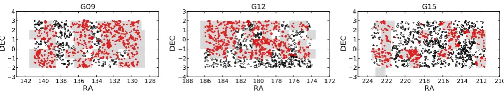
Figure 1. KiDS-ESO-DR1/2 coverage of the three equatorial GAMA fields (G09, G12, G15). Each grey box corresponds to a single KiDS tile of 1 deg2_{. The}

black circles represent groups withNfof≥5 in the G3Cv7 catalogue (R+11). The size of the dots is proportional to the group apparent richness. The filled

red circles indicate the groups used in this analysis. These are all groups either inside a KiDS field or whose centre is separated less than 2h−1_{Mpc from the}

centre of the closest KiDS field.

Table 1. Summary of the area overlap of KiDS-DR1/2 in the three GAMA fields and the number of groups with at least five members used in this analysis. In parenthesis we quote the effective area, accounting for masks, used in this work.

GAMA field KiDS-DR1/2 overlap (deg2_{) Number of groups}

G09 44.0 (28.5) 596

G12 36.0 (25.0) 509

G15 20.0 (15.0) 308

Figure 2. Redshift distribution of the GAMA groups used in this analy-sis (red histogram) and the KiDS galaxies (blue lines). In the case of the GAMA groups, we use the spectroscopic redshift of the groups with at least five members (R+11), while for the KiDS galaxies the redshift distribu-tion is computed as a weighted sum of the posterior photometric redshift distribution as provided by BPZ (Ben´ıtez2000). The weight comes from lensfit, used to measure the shape of the objects (Miller et al.2007). The two vertical lines show the median of the redshift distribution of the GAMA groups and of the KiDS sources. The two peaks in the redshift distribution of the GAMA groups are physical (and not caused by incompleteness), due to the clustering of galaxies in the GAMA equatorial fields.

the equatorial region, which allows for the identification of a large number of galaxy groups.

Fig.1shows the KiDS-DR1/2 coverage of the G09, G12, and G15 GAMA fields. We also show the spatial distribution of the galaxy groups in the three GAMA fields (open black circles) and the selection of groups entering in this analysis (red filled circles).

Table1lists the overlap between KiDS-DR1/2 and GAMA and the total number of groups used in this analysis. Fig. 2 shows the redshift distribution of the GAMA groups used in this work

and of the KiDS source galaxies, computed as a weighted sum of the posterior photometric redshift distribution as provided by BPZ (Ben´ıtez2000). The weight comes from thelensfit code, which is used to measure the shape of the objects (Miller et al.2007, see Sec-tion 3.2.1). The median redshift of the GAMA groups isz=0.2, while the weighted median redshift of KiDS is 0.53. The multiple peaks in the redshift distribution of the KiDS sources result from degeneracies in the photometric redshift solution. This is discussed further inK+15. The different redshift distributions of the two sur-veys are ideal for a weak lensing study of the GAMA groups using the KiDS galaxies as background sources.

3.1 Lenses: GAMA Groups

One of the main products of the GAMA survey is a group catalogue, G3_{C (R+11), of which we use the internal version 7. It consists of}

23 838 galaxy groups identified in the GAMA equatorial regions (G09, G12, G15), with over 70 000 group members. It has been constructed employing spatial and spectroscopic redshift informa-tion (Baldry et al.2014) of all the galaxies targeted by GAMA in the three equatorial regions. The groups are found using a friends-of-friends algorithm, which links galaxies based on their projected and line-of-sight proximity. The choice of the linking length has been optimally calibrated using mock data (R+11; Merson et al.

2013) based on the Millennium simulation5_{(Springel et al.2005b)}

and a semi-analytical galaxy formation model (Bower et al.2006). Running the final group selection algorithm on the mock catalogues shows that groups with at least five GAMA galaxies are less affected by interlopers and have sufficient members for a velocity dispersion estimate (R+11). For this reason we use only such groups in our analysis. This choice leaves us with 1413 groups, in KiDS-DR1/2, 11 per cent of the full GAMA group catalogue.

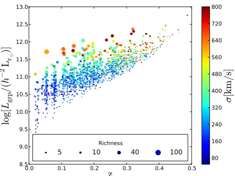
Fig.3shows the distribution of the total groupr-band luminosity as a function of the redshift of the group, the group apparent rich-ness, which is the number of members brighter thatr=19.8, and the group velocity dispersion corrected for velocity uncertainty, for this subsample. These groupr-band luminosity values are calcu-lated by summing ther-band luminosity of all galaxies belonging to a group and targeted by GAMA and they also include an es-timate of the contribution from faint galaxies below the GAMA flux limit, as discussed inR+11. This correction is typically very small, a few per cent at low redshift and a factor of a few atz∼0.5 since most of the luminosity comes from galaxies aroundM −

5 logh∼ −20.44 (Loveday et al.2012, 2015), and most of the

5₍

Figure 3. Total groupr-band luminosity as a function of the redshift of the group. The size of the points is proportional to the group apparent richness and the colour of the points indicates the group velocity dispersion corrected for velocity uncertainty. The shape of the distribution is typical of a flux limited survey.

groups are sampled well belowM. Note that all absolute magni-tudes and luminosities used in the paper arek-corrected and evo-lution corrected at redshiftz=0 (R+11). The globalk-correction used byR+11 is compatible with the mediank-correction of the full GAMA (McNaught-Roberts et al.2014, fig.1in the paper).

All the stellar masses used in this work are taken from Taylor et al. (2011), who fitted Bruzual & Charlot (2003) synthetic stellar spectra to the broad-band Sloan Digital Sky Survey (SDSS) photometry assuming a Chabrier (2003) IMF and a Calzetti et al. (2000) dust law.

3.2 Sources: KiDS galaxies

We measure the gravitational lensing effect induced by the GAMA groups using galaxy images from KiDS. We refer toK+15for a detailed description of the pipelines used to measure shapes and photometric redshifts for those objects. We briefly summarize here the aspects of the data processing most relevant for this analysis.

3.2.1 Shape measurements

All of our lensing measurements are derived from ther-band ex-posures in KiDS. This is the band with the highest image quality of the survey, as the queue-scheduling at the telescope ensures that observations in this filter are taken in the best seeing conditions. The images are processed with theTHELIpipeline, which has been

optimized for lensing applications (Erben et al.2013), and elliptic-ities for the galaxies are derived using thelensfit code (Miller et al.

2007,2013; Kitching et al.2008).lensfit takes full account of the point spread function (PSF) in the individual (dithered) exposures and prior knowledge of the ellipticity and size distributions of faint galaxies, returning an ellipticity estimate for each galaxy as well as an inverse variance weight that is related to the uncertainty of the measurement.

The average number density of galaxies withlensfit weightw larger than 0, and satisfying the photometric redshift cuts described

in the next section, is 8.88 arcmin−2_{, corresponding to an effective}

number density:

neff= σ2s

A

i

wi (7)

of 4.48 galaxies per square arcmin, whereAis the survey area and

σ2

s=0.065 is the intrinsic ellipticity variance. This is a

measure-ment of the statistical power of the weak lensing data (see Chang et al.2013andK+15for more details).

It is well known that shape measurements for galaxies with low signal-to-noise ratio and small sizes tend to be biased (e.g. Melchior & Viola 2012; Refregier et al. 2012; Miller et al. 2013; Viola, Kitching & Joachimi2014). This ‘noise-bias’ stems from the non-linear transformations of the image pixels involved in the derivation of galaxy image shapes. It has the form of a multiplicative bias, and a calibration of the shape measurements is typically required in order to get an unbiased shear estimator. In this paper, we use the same calibration that was determined in Miller et al. (2013). This calibration depends on the signal-to-noise and the size of the objects and needs to be applied, in an average sense, to the recovered shear field. In addition to this multiplicative bias, shape measurements can also be affected by an additive bias caused by a non-perfect PSF deconvolution, centroid bias and pixel level detector effects. This bias can be empirically quantified and corrected for directly from the data, using the residual average ellipticity over the survey area. More detail on these ∼10 per cent bias corrections can be found inK+15.

The analysis presented in this paper has been applied to four different ellipticity catalogues. Three of these catalogues were gen-erated by rescaling all the ellipticity measurements by some fac-tors unknown to the team and chosen by a colleague, Matthias Bartelmann,6 _{external to the collaboration. The amplitude of the}

rescaling has been chosen such that the cosmological parameters derived from a cosmic shear analysis using the four blind catalogues would not differ more than 10σ, where sigma is the error from the Planck cosmological papers. We refer to this procedure as blind-ing, and we have used it to mitigate confirmation bias in our data analysis. The authors asked our external tounblindthe true shear catalogues only just before paper submission. The authors were not allowed to change any of the results after the unblinding, without documenting those changes. Whilst the shear was blind, we did not blind measurements of group properties, such as their luminosity, or measurements of the source photometric redshifts.

3.2.2 Photometric redshift measurements

The observable lensing distortion depends on the distances to the lens and source (equation 6). Redshifts to the lenses are known from the GAMA spectroscopy, but for the sources we need to resort to photometric redshifts derived from the KiDS-ESO-DR1/2 ugri images in the ESO data release. Processing and calibration of these images is done using the Astro-WISE environment (McFarland et al.2013), and flux and colour measurements use the ‘Gaussian Aperture and Photometry’ technique designed to correct aperture photometry for seeing differences (Kuijken2008). These colours form the basis of the photometric redshift estimates, obtained with BPZ (Ben´ıtez2000; Hildebrandt et al.2012). After extensive tests, we reject galaxies whose photometric redshift posterior distribution

p(z) peaks outside the range [0.005,1.2] (K+15). In what follows thep(z) for each source is used in the calculation of distances, and in particular in the calculation of the critical surface density (see equation 6).K+15show that if the peak of each source’sp(z) had been used as the estimate of the redshift, the average value ofcr and hence the average ESD would have been underestimated by

∼10 per cent .

3.3 Measurement of the stacked ESD profile

The shape measurement algorithm used in this work,lensfit, pro-vides measurements of the galaxy ellipticities (1,2) with respect to an equatorial coordinate system.

For each source–lens pair, we compute the tangentialtand cross componentxof the source’s ellipticity around the position of the lens,

t x

=

−cos(2φ) −sin(2φ) sin(2φ) −cos(2φ)

1 2

, (8)

whereφis the position angle of the source with respect to the lens. The average of the tangential ellipticity of a large number of galaxies in the same area of the sky is an unbiased estimate of the shear. On the other hand, the average of the cross ellipticity over many sources should average to zero. For this reason, the cross-ellipticity is commonly used as an estimator of possible systematics in the measurements. Each lens-source pair is then assigned a weight

˜

wls=ws˜−2

cr , (9)

which is the product of thelensfit weightwsassigned to the given source ellipticity, and a geometric term ˜cr which downweights lens-source pairs that are close in redshift and therefore less sensitive to lensing. We compute the ‘effective critical surface density’ for each pair from the spectroscopic redshift of the lenszland the full posterior redshift distribution of the source,p(zs):

˜

−1 cr =

4πG

c2 _∞

zl

Dl(zl)Dls(zl, zs)

Ds(zs) p(zs) dzs. (10) Finally, following equation (5), we compute the ESD in bins of projected distanceRto the lenses:

(R)=

⎛

⎝ lswlst˜ cr˜ lswls˜

⎞

⎠ 1

1+K(R), (11)

where the sum is over all source–lens pairs in the distance bin, and

K(R)= lswlsms˜

lswls˜

, (12)

is an average correction to the ESD profile that has to be applied to correct for the multiplicative noise bias min the lensfit shear estimates. Typically, the value of theK(R) correction is around 0.1, largely independent of the scale at which it is computed.

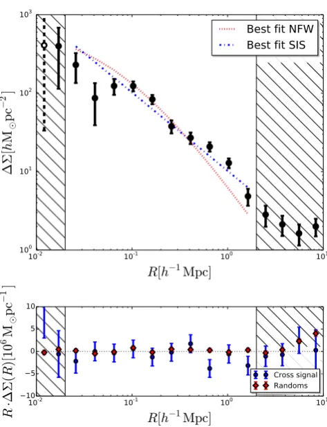
Fig.4shows the stacked ESD profile for all groups either inside a KiDS field or whose centre is separated by less than 2h−1_{Mpc from}

the centre of the closest KiDS field. It shows a highly significant detection of the lensing signal (signal-to-noise ratio∼120). We note that the signal to noise is very poor at scales smaller than 20h−1_kpc.

This is due to the fact that many objects close to the group centres are blended, andlensfit assigns them a vanishing weight. We exclude those scales from any further analysis presented in this paper.

For reference, we also show the best-fitting singular isothermal sphere (SIS) andNFWmodels to the stacked ESD signal. In the

Figure 4. Top panel: ESD profile measured from a stack of all GAMA groups with at least five members (black points). Here, we choose the BCG as the group centre. The open white circle with dashed error bars indicates a negative. The dotted red line and the dash–dotted blue line show the best fits to the data ofNFW(Navarro et al.1995) and SIS profiles, respectively. Neither of the single-parameter models provides a good fit to the data, highlighting that complex modelling of the signal is required. Bottom panel: ESD profile, multiplied byRto enhance features at large radii, measured from the cross-component of the ellipticities for these same groups (blue points) and measured around random points using the same redshift distribution of the groups (red points). We only use measurements at scales outside the dashed areas for the rest of the paper.

case of theNFWmodel, the halo concentration is fixed using the Duffy et al. (2008) mass–concentration relation. Neither of the two single-parameter models provides a good fit to the data (χ2

red>2.5),

highlighting how a more complex modelling of the signal is required (see Section 4).

Fig. 4also includes two tests for residual systematic errors in the data: the cross-component of the signal and the signal mea-sured around random points in the KiDS tiles. On scales larger than 2h−1_{Mpc, small but significant deviations are evident. We believe}

that one possible origin of the non-vanishing signal around random points at these scales is due to the incomplete azimuthal average of galaxy ellipticities, but we cannot exclude some large-scale sys-tematics in the shear data. The current patchy coverage of lensing data complicates a detailed analysis and here we simply note that the effect is small (less than 10 per cent of the signal at 2h−1_Mpc)

and exclude data on scales larger than 2h−1_{Mpc. Future analyses}

based on more uniform coverage of the GAMA area from the KiDS survey will need to address these potential issues.

Figure 5. Left panel: ESD correlation matrix between different radial bins estimated from the data. This matrix accounts for shape noise and the effect of the mask and is computed as described in Section 3.4. Middle panel: ESD correlation matrix between different radial bins estimated using a bootstrap technique. It accounts for cosmic variance as well as shape noise. Right panel: comparison of the square root of the diagonal elements of the two covariance matrices as a function of distance from the group centre (here the BCG). Note the lower noise in the left-hand panel and the small but significant correlation between the largest-radial bins, which is a consequence of the many survey edges.

of the shear and the signal around random points are consistent with a null-detection over these scales.

3.4 Statistical error estimate

In a stacking analysis with many foreground lenses, the ellipticity of any source galaxy can contribute to theiestimate in multiple

radial binsiof different lenses. We summarize here how we compute the resulting covariances between the ESD estimatesifrom the

data.

We start from equation (11), which gives the expression fori.

For simplicity, we drop in what follows the noise bias correction factor 1+K(R) as it can be considered to have been absorbed in the effective critical density ˜cr.

We first rearrange the sum in equation (11) to separate the con-tributions from each source s, by summing first over all lenses l that project within the radial binifrom source s; for each sourceswe denote this set of lenses asis. We can then rewrite equation (11) as

i= sws(1sCsi+2sSsi) swsZsi

, (13)

whereC,S, andZare sums over the lenses

Csi=

l∈is

−˜−1

cr,lscos(2φls), (14)

Ssi=

l∈is

−˜−1

cr,lssin(2φls), (15)

and

Zsi=

l∈is

˜

−2

cr,ls. (16)

Since eachksis an independent estimate of the shear field, where k=1,2, the ESD covariance between radial binsiandjcan then be easily written as

Covij = sσ 2 w2s

CsiCsj+SsiSsj

( swsZsi)( swsZsj)

, (17)

whereσ2

=0.078 is the ellipticity dispersion weighted with the lensfit weight, for one component of the ellipticity. We compute this number from the whole KiDS-ESO-DR1/2 area.

Equation (17) can be generalized to also compute the covari-ance between the ESD estimates for two different lens samples

mandn:

Covmnij= sσ 2 ws2

Csi,mCsj,n+Ssi,mSsj,n

( _swsZs_i,m)( _swsZs_j,n) , (18)

by restricting the sums for theC,S, andZterms to lenses in the relevant samples.

We test the accuracy of the above calculation, which does not account for cosmic variance, against the covariance matrix obtained via a bootstrapping technique. Specifically, we bootstrap the signal measured in each of the 1 deg2_{KiDS tiles. We limit the comparison}

to the case in which all groups are stacked together7_{and compute the}

signal in 10 logarithmically spaced radial bins between 20h−1_kpc

and 2h−1_{Mpc. This leads to an ESD covariance matrix with 55}

independent entries, which can be constrained by the 100 KiDS tiles used in this analysis. The corresponding matrix is shown in Fig.5together with the correlation matrix obtained from equation (17). The small but significant correlation between the largest radial bins is a consequence of the survey edges. We further show the diagonal errors obtained with the two methods, labelled Analytical and Bootstrap. Based on the work by Norberg et al. (2009), we might expect that the bootstrapping technique leads to somewhat larger error bars, although on larger scales this trend may be counteracted to some degree by the limited independence of our bootstrap regions. However, the conclusions of Norberg et al. (2009) are based on an analysis of galaxy clustering, and a quantitative translation of their results to our galaxy–galaxy lensing measurements is not easy and beyond the scope of this work. The difference between the error estimates using these two independent methods is at most 10 per cent at scales larger than 300h−1_{kpc. Based on the results of}

this test, we consider the covariance matrix estimated from equa-tion (17) to be a fair estimaequa-tion of the true covariance in the data, and we use it throughout the paper. In our likelihood analyses of various models for the data (see next section), we account for the covariance between the radial bins as well as between the different lens samples used to compute the stacked signal. We note that future analyses with greater statistical power, for example those based on the full KiDS and GAMA overlap, and studies focusing on larger scales than those considered in this analysis, will need to properly

7_{If the signal is split further into several bins according to some property}

evaluate the full covariance matrix that incorporates the cosmic variance contribution that is negligible in this work.

4 H A L O M O D E L

In this section, we describe the halo model (e.g. Seljak2000; Cooray & Sheth2002), which we use to provide a physical interpretation of our data. We closely follow the methodology introduced in van den Bosch et al. (2013) and successfully applied to SDSS galaxy–galaxy lensing data in Cacciato et al. (2013).

This model provides the ideal framework to describe the statis-tical weak lensing signal around galaxy groups. It is based on two main assumptions:

(i) a statistical description of dark matter halo properties (i.e. their average density profile, their abundance, and their large scale bias);

(ii) a statistical description of the way galaxies with different observable properties populate dark matter haloes.

As weak gravitational lensing is sensitive to the mass distribution projected along the line of sight, the quantity of interest is the ESD profile, defined in equation (3), which is related to the galaxy– matter cross-correlation via equation (2). Under the assumption that each galaxy group resides in a dark matter halo, its average

(R,z) profile can be computed using a statistical description of how galaxies are distributed over dark matter haloes of dif-ferent mass and how these haloes cluster. Specifically, it is fairly straightforward to obtain the two-point correlation function,ξgm(r,

z), by Fourier transforming the galaxy–dark matter power-spectrum,

Pgm(k,z), i.e.

ξgm(r, z)= 1 2π2

∞

0

Pgm(k, z)sin(kr)

kr k2dk , (19)

withkthe wavenumber, and the subscript ‘g’ and ‘m’ standing for ‘galaxy’ and ‘matter’.

In what follows, we will use the fact that, in Fourier space, the matter density profile of a halo of mass M at a redshift z can be described as Muh˜ (k|M, z), whereM≡4π(200 ¯ρ)R3_{200/3, and}

˜

uh(k|M) is the Fourier transform of the normalizeddarkmatter density profile of a halo of massM.8_{We do not explicitly model the}

baryonic matter density profile (Fedeli2014) because, on the scales of interest, its effect on the lensing signal can be approximated as that of a point mass (see Section 4.1). Because the lensing signal is measured by stacking galaxy groups with observable property

Ogrp, on scales smaller than the typical extent of a group, we have

Pgm(k, z)=P1h

grp m(k, z), where

P1h

grp m(k, z)=

P(M|Ogrp)Hm(k, M, z) dM , (20)

and

Hm(k, M, z)≡ M ¯

ρmuh˜ (k|M, z), (21)

with ¯ρmthe comoving matter density of the Universe. Throughout the paper, the subscript ‘grp’ stands for ‘galaxy group’.

The functionP(M|Ogrp) is the probability that a group with observable propertyOgrpresides in a halo of massM. It reflects the halo occupation statistics and it can be written as

P(M|Ogrp) dM=Hgrp(M, z)nh(M, z) dM . (22)

8_{We useM}

200masses for the groups throughout this paper, i.e. as defined

by 200 times the mean density (and corresponding radius, noted asR200).

Here, we have used

Hgrp(M, z)≡ NOgrp(M) ¯

ngrp(Ogrp, z), (23) where,N_Ogrp(M) is the average number of groups with observable propertyOgrpthat reside in a halo of massM.

Note thatnh(M,z) is the halo mass function (i.e. the number den-sity of haloes as a function of their mass) and we use the analytical function suggested in Tinker et al. (2008) as a fit to a numerical

N-body simulation. Furthermore, the comoving number density of groups, ¯ngrp, with the given observable property is defined as

¯

ngrp(Ogrp, z)=

NOgrp(M)nh(M, z) dM . (24)

Note that in the expressions above, we have assumed that we can correctly identify the centre of the galaxy group halo (e.g. from the position of the galaxy identified as the central in the GAMA group catalogue). In Section 4.1, we generalize this expression to allow for possiblemis-centringof the central galaxy.

Galaxy groups are not isolated, and on scales larger than the typ-ical extent of a group, one expects a non-vanishing contribution to the power spectrum due to the presence of other haloes surrounding the group. This term is usually referred to as the two-halo term [as opposed to the one-halo term described in equation (20)]. One thus has

Pgm(k)=Pgrp m1h (k)+P 2h

grp m(k). (25)

These terms can be written in compact form as

P1h

grp m(k, z)=

Hgrp(k, M, z)Hm(k, M, z)nh(M, z) dM, (26)

P2h

grp m(k, z)=

dM1Hgrp(k, M1, z)nh(M1, z)

×

dM2Hm(k, M2, z)nh(M2, z)Q(k|M1, M2, z). (27)

The quantity Q(k|M1, M2, z) describes the power spectrum of haloes of massM1andM2. In its simplest implementation,9_used

throughout this paper, Q(k|M1, M2, z) ≡ bh(M1, z)bh(M2, z)Plin

(k,z), wherebh(M,z) is the halo bias function andPlin_{(k,z) is the}

linear matter–matter power spectrum. We note that, in the literature, there exist various fitting functions to describe the mass dependence of the halo bias (see for example Sheth & Tormen1999; Sheth, Mo & Tormen2001; Tinker et al.2010). These functions may exhibit differences of up to∼10 per cent (e.g. Murray, Power & Robotham

2013). However, a few points are worth a comment.

First, the use of the fitting function from Tinker et al. (2010) is motivated by the use of a halo mass function calibrated over the same numerical simulation. Secondly, the halo bias function enters in the galaxy–matter power spectrum only through the two-halo term and as part of an integral. Thus, especially because we will fit the ESD profiles only up toR=2h−1_{Mpc, the uncertainty related}

to the halo bias function is much smaller than the statistical error associated with the observed signal.

4.1 Model specifics

The halo occupation statistics of galaxy groups are defined via the functionN_Ogrp(M), the average number of groups (with a

9_{See for example, van den Bosch et al. (2013) for a more refined description}

given observable property Ogrp, such as a luminosity bin) as a function of halo massM. Since the occupation function of groups as a function of halo mass,Ngrp(M), is either zero or unity, one has thatN_Ogrp(M) is by construction confined between zero and

unity. We model N_Ogrp(M) as a lognormal characterized by a mean, log[ ˜M/(h−1_M

)], and a scatterσlog ˜M:

NOgrp(M)∝

1

√

2πσlog ˜_Mexp

−(logM−log ˜M)2

2σ2 log ˜M

. (28)

We caution the reader against overinterpreting the physical meaning of this scatter; this number mainly serves the purpose of assigning a distribution of masses around a mean value.

Ideally, for each stack of the group ESD (in bins of group lu-minosity or total stellar mass) we wish to determine both these parameters, but to keep the number of fitting parameters low we assume here thatσlog ˜_Mis constant from bin to bin, with a flat prior 0.05≤σlog ˜_M ≤1.5. This prior does not have any statistical effect on the results and it only serves the purpose of avoiding numerical in-accuracies. There is evidence for an increase in this parameter with central galaxy luminosity or stellar mass, (e.g. More et al.2009a,b,

2011), but these increases are mild, and satellite kinematics (e.g. More et al. 2011) support the assumption thatσlog ˜_M is roughly constant on massive group scales (i.e. log [M/(h−1_M

)]>13.0). We have verified that our assumption has no impact on our results in terms of either accuracy or precision by allowingσlog ˜_M to be different in each observable bin.

For each given bin in an observable group property, one can define an effective mean halo mass,M, as

MOgrp ≡

P(M|Ogrp)MdM

=

NOgrp(M)nh(M,z¯)MdM

¯

ngrp(Ogrp,z¯) , (29) where ¯zis the mean redshift of the groups in the bin under considera-tion, and we have made use of equations (22) and (24). The effective mean halo mass,M_Ogrp, is therefore obtained as a weighted

av-erage where the weight is the multiplication of the halo occupation statistics and the halo mass function.

The dark matter density profile of a halo of massM,ρm(r|M), is assumed to follow anNFWfunctional form

ρm(r|M)= δ ρ

(r/rs)(1+r/rs)2, (30)

wherers is the scale radius andδ is a dimensionless amplitude which can be expressed in terms of the halo concentration parameter

cm≡R200/rsas

δ= 200

3

c3 m

ln(1+cm)−cm/(1+cm), (31)

where the concentration parameter, cm, scales with halo mass. Different studies in the literature have proposed somewhat dif-ferent fitting functions (e.g. Bullock et al.2001; Eke, Navarro & Steinmetz2001; Duffy et al.2008; Macci`o, Dutton & van den Bosch

2008; Klypin, Trujillo-Gomez & Primack2011; Prada et al.2012; Dutton & Macci`o2014) to describe the relationcm(M,z). Overall, these studies are in broad agreement but unfortunately have not converged to a robust unique prediction. Given that those fitting functions have been calibrated using numerical simulations with very different configurations (most notably different mass resolu-tions and cosmologies), it remains unclear how to properly account for the above mentioned discrepancies. As these fitting functions

all predict a weak mass dependence, we decide to adopt an effec-tive concentration–halo mass relation that has the mass and redshift dependence proposed in Duffy et al. (2008) but with a rescalable normalization:

ceff

m(M200, z)=fc×c Duffy m (M200, z)

=fc×10.14

M200

2×1012 −0.081

(1+z)−1.01_{. (32)}

Note that at z = 0.25, one hascDuffy

m ≈5 for halo masses with

log [M/(h−1_M

)]≈ 14.3. We leavefc free to vary within a flat uninformative prior 0.2≤fc≤5.

The innermost part of a halo is arguably the site where a ‘central’ galaxy resides. The baryons that constitute the galaxy may be dis-tributed according to different profiles depending on the physical state (for example, exponential discs for stars and β-profiles for hot gas; see Fedeli2014). The lensing signal due to these different configurations could in principle be modelled to a certain level of sophistication (see Kobayashi et al.2015). However, at the smallest scales of interest here,10 _{those distributions might as well be}

ac-counted for by simply assuming a point mass,MP. In the interest of simplicity, we assume that the stellar mass of the brightest cluster galaxy (MBCG

; Taylor et al.2011) is a reliable proxy for the amount

of mass in the innermost part of the halo. Specifically, we assume that

MP=APMBCG

, (33)

whereAPis a free parameter, within a flat prior between 0.5 and 5. The adopted definition of centre may well differ from the true minimum of the gravitational potential well. Such a mis-centring of the ‘central’ galaxy is in fact seen in galaxy groups (see e.g. Skibba & Macci`o2011and references therein). George et al. (2012) offer further independent support of such a mis-centring, finding that massive central galaxies trace the centre of mass to less than 75 kpch−1_.

We model this mis-centring in a statistical manner (see also Oguri & Takada 2011; Miyatake et al. 2015; More et al. 2015

and references therein). Specifically, we assume that the degree of mis-centring of the groups in three dimensions,(M, z), is pro-portional to the halo scale radiusrs, a function of halo mass and redshift, and parametrize the probability that a ‘central’ galaxy is mis-centred aspoff. This gives

Hgrp(k, M,z¯)= NOgrp(M) ¯

ngrp(¯z) (1−poff+poff×e

[−0.5k2_(r sRoff)2]₎.

(34)

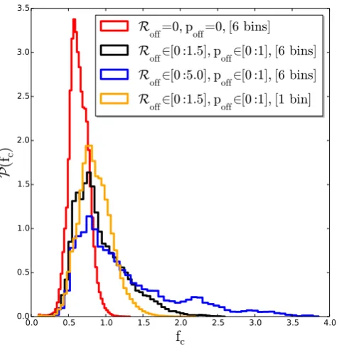
Setting either poff or Roff to zero implies that there is de facto no offset. We treat the two as free parameters in Section 5. The parameterpoff, being a probability, is bound between zero and unity. We apply a flat uniform prior toRoff ∈[0,1.5]. We note that this prior is very conservative, as according to George et al. (2012) and Skibba & Macci`o (2011) the mis-centring is expected to be smaller than the scale radius of a group, for whichRoff=1.

In summary, the model parameter vector, is defined as λ= (log ˜M_i, σlog ˜M, fc, AP, poff,Roff) wherei=1, . . . ,Nbins. Through-out the paper, we bin group observable properties in six bins. This leads to an 11-parameter model. We use Bayesian inference tech-niques to determine the posterior probability distributionP(λ|D) of the model parameters given the data,D. According to Bayes’

Table 2. Summary of the bin limits used to compute the stacked ESD signal, the number of groups in each bin, the mean redshift of the groups in each bin and the mean stellar mass of the BCG.

Observable Bin limits Number of lenses Mean redshift log(MBCG

[h−2M])

log [Lgrp/(h−2L)] (9.4, 10.9, 11.1, 11.3, 11.5, 11.7, 12.7) (540, 259, 178, 233, 142, 66) (0.13, 0.20, 0.23, 0.26, 0.30, 0.35) (11.00, 11.23, 11.29, 11.37, 11.47, 11.70) σ /(s−1_{km) (0, 225, 325, 375, 466, 610, 1500) (501, 359, 124, 198, 147, 89) (0.15, 0.19, 0.21, 0.23, 0.26, 0.31) (11.05, 11.20, 11.30, 11.36, 11.41, 11.64)} Nfof (5, 6, 7, 8, 11, 19, 73) (481, 261, 170, 239, 181, 86) (0.21, 0.21, 0.21, 0.19, 0.18, 0.16) (11.17, 11.23, 11.29, 11.29, 11.35, 11.45) LBCG/Lgrp (1.0, 0.35, 0.25, 0.18, 0.13, 0.08, 0) (346, 252, 296, 227, 200, 97) (0.10, 0.16, 0.20, 0.25, 0.29, 0.34) (11.16, 11.19, 11.22, 11.29, 11.36, 11.53)

theorem,

P(λ|D)∝P(D|λ)P(λ)∝exp

−χ2_(λ)

2

P(λ), (35)

whereP(D|λ) is the likelihood of the data given the model param-eters, assumed to be Gaussian, andP(λ) is the prior probability of these parameters. Here,

χ2

(λ)=[k,j−k,j]T(C−1)kk,jj[k,j −k,j], (36)

where k,j is thej’th radial bin of the observed stacked ESD

for the groups in bin k, and _k,j is the corresponding model prediction.Cis the full covariance matrix for the measurements, computed as detailed in Section 3.4.

We sample the posterior distribution of our model parameters given the data using a Markov Chain Monte Carlo (MCMC). In particular, we use11 _{a proposal distribution that is a multivariate}

Gaussian whose covariance is computed via a Fisher analysis run during the burn-in phase of the chain, set to 5000 model evaluations.

5 D E N S I T Y P R O F I L E O F G A L A X Y G R O U P S

We measure the ESD signal around each GAMA group with at least five members in 10 logarithmically-spaced radial bins in the range 20h−1_kpc–2h−1_{Mpc. We first assign errors to those measurements}

by propagating the shape noise on the tangential shear measurement in each radial bin. We divide the groups into six bins according to a given observable property, such as their velocity dispersion, total

r-band luminosity, apparent richness orr-band luminosity fraction of the BCG. Bin limits are chosen to make the signal to noise of the ESD roughly the same in each bin. Once the bin limits are defined, we compute the data covariance between radial bins and between group bins as outlined in Section 3.4. We summarize the bin-limits, the number of groups in each bin, the mean redshift of the bin and the mean stellar mass of the BCG in Table2for the four observables considered in this work.

The typical signal-to-noise ratio in each of the six luminosity bins is of the order of∼20–25. This is comparable to the signal-to-noise ratio reported by Sheldon et al. (2009) for a weak lensing analysis of

∼130 000 MaxBCG clusters using SDSS imaging, once we restrict the comparison to a similar luminosity range.

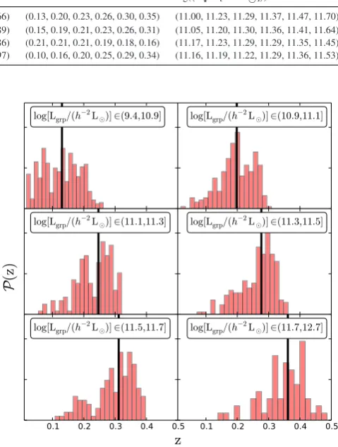
We jointly fit the signal in the six bins using the halo model described in Section 4. Since GAMA is a flux limited survey, the redshift distributions of the groups in the six luminosity bins are different, as shown in Fig.6. When we fit the halo model to the data, we calculate the power spectra and mass function (equations 20–27) using the median of the redshift distribution in each bin.

For each observable property, we run five independent chains with different initial conditions. We evaluate the convergence of the

11_{A python implementation of this sampling method is available via the} MONTEPYTHONcode thanks to the contribution by Surhud More.

Figure 6. Redshift distributions of the GAMA groups used in this paper in the sixr-band luminosity bins. The group luminosity increases from left to right and from top to bottom. The solid vertical black lines indicate the median of the distributions.

MCMC by means of a Gelman Rubin test (Gelman & Rubin1992), and we imposeR<1.03, where theR-metric is defined as the ratio of the variance of a parameter in the single chains to the variance of that parameter in an ‘¨uber-chain’, obtained by combining five chains.

5.1 Matter density profiles of group-scale haloes

We first test whether the ESD measurements themselves support the halo model assumption that the group density profile can be described in terms of a mis-centredNFWprofile with a contribu-tion from a point mass at small scales, and what constraints can be put on the model parameters. In the interest of being concise, we only present the results derived by binning the groups according to their totalr-band luminosity (see Section 3), as statistically equiv-alent results are obtained when the groups are binned according to their velocity dispersion, apparent richness orr-band luminosity fraction of the BCG. The binning by other observables will become important in the study of scaling relation presented in Section 6.

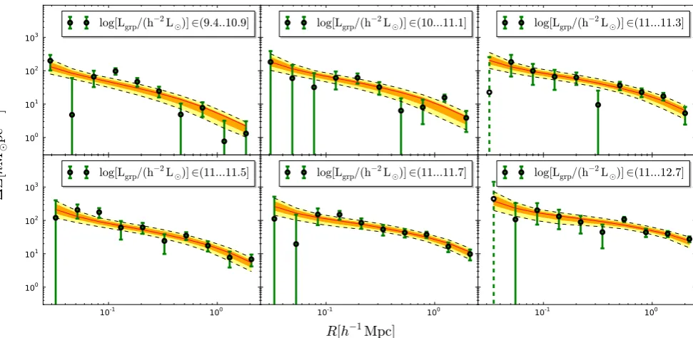
Figure 7. Stacked ESD profile measured around the groups BCG of the six group luminosity bins as a function of distance from the group centre. The group r-band luminosity increases from left to right and from top to bottom. The stacking of the signal has been done using only groups withNfof≥5. The error bars

on the stacked signal are computed as detailed in Section 3.4 and we use dashed bars in the case of negative values of the ESD. The orange and yellow bands represent the 68 and 95 percentile of the model around the median, while the red line shows the best-fitting model.

Throughout the paper, unless stated otherwise, we use theBCGas the definition of the centre, as it is a common choice in the literature. We investigate the effect of using the other two definitions of the group centre in Section 5.1.4 and in Appendix A.

Fig.7shows the stacked ESD profiles (green points with error bars) for the six bins in totalr-band luminosity. Note that the error bars are the square root of the diagonal elements of the full covari-ance matrix, and we use dashed bars in the case of negative values of the ESD. The ESD profiles have high signal to noise through-out the range in total luminosity and in spatial scales. Red lines indicate the best-fitting model, whereas orange and yellow bands indicate the 68 and 95 per cent confidence interval. The model de-scribes the data well with a reducedχ2

red=1.10, 49 d.o.f, over

the full scale range, for all the luminosity bins. This justifies our assumption that the ESD profile can be accurately modelled as a weighted stack of mis-centredNFWdensity profiles with a contri-bution from a point mass at the centre.

The main results of this analysis can be summarized as follows (68 per cent confidence limits quoted throughout).

(i) For each r-band luminosity bin, we derive the probability that a group with that luminosity resides in a halo of massM(see equation 22). We show the median of the probability distribution for the six bins in Fig.8. We constrain the scatter in the mass at a fixed total r-band luminosity to be σlog ˜_M =0.74₋+00..0916. This

sets the width of the lognormal distribution describing the halo occupation statistics. We remind the reader thatσlog ˜_Mis the width of the distribution in halo masses at given total luminosity of the groups and it isnotthe scatter in luminosity (or stellar mass) at a fixed halo mass that is often quoted in the literature and that one would expect to be considerably smaller (e.g. Cacciato et al.2009; Yang, Mo & van den Bosch2009; More et al.2011; Leauthaud et al.

2012a). This hampers the possibility of a one-to-one comparison

with most studies in the literature. However, we note that van den Bosch et al. (2007) and More et al. (2011) reported values of the

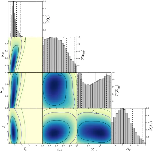
Figure 9. Posterior distribution of the normalization of the mass-concentration relationfc, of the mis-centring parameterspoffandRoffand of the amplitude

of the point mass AP. The contours indicate the 1σ, 2σ, 3σconfidence regions. The dashed vertical lines and the dotted vertical lines correspond, respectively,

to the 1σand 2σmarginalized confidence limits .These are the constraints from a joint halo model fit of the ESD signal in the six luminosity bins usingBCG as the group centre. The range in each panels reflect the priors used for the different parameters.

scatter in halo mass at fixed luminosity that are as high as 0.7 at the bright end. Furthermore, More et al. (2015) reported a value of 0.79+₋0₀._.41₃₉ for the width of the low-mass end distribution of the halo occupation statistics of massive CMASS galaxies. Given the non-negligible differences between the actual role of this parameter in all these studies, we find this level of agreement satisfactory.

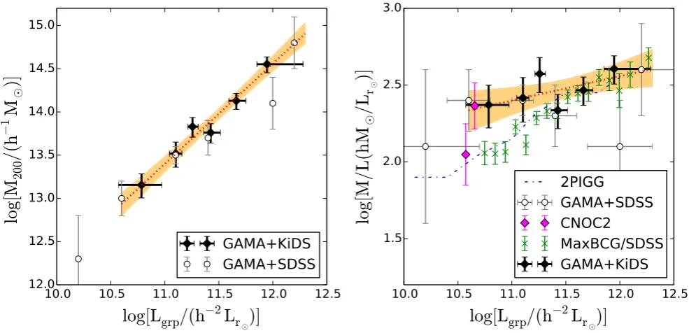
(ii) For each luminosity bin, a mean halo mass is inferred with a typical uncertainty on the mean of∼0.12 dex.

(iii) The relative normalization of the concentration–halo mass relation (see equation 32) is constrained to befc=0.84+₋0₀._.42₂₃, in agreement with the nominal value based on Duffy et al. (2008).

(iv) The probability of having an off-centred BCG ispoff<0.97 (2σ upper limit), whereas the average amount of mis-centring in terms of the halo scale radius,Roff, is unconstrained within the prior.

(v) The amount of mass at the centre of the stack which con-tributes as a point mass to the ESD profiles is constrained to be

MPM=APMMBCG =2.06₋+01..1999MBCG.

Table 3. Constraints on the average halo mass in eachr-band luminosity bin using the three definitions of halo centre. We quote here the median of the mass posterior distribution, marginalized over the other halo model parameters, and the errors are the 16th and 84th percentile of the distribution. All of the constraints derived using the three different proxies for the halo centre agree within 1σ.

Centre log[M₂₀₀(1)/(h−1_M

)] log[M₂₀₀(2)/(h−1_M

)] log[M₂₀₀(3)/(h−1_M

)] log[M₂₀₀(4)/(h−1_M

)] log[M₂₀₀(5)/(h−1_M

)] log[M₂₀₀(6)/(h−1_M

)] BCG 13.15₋+₀0._.13₁₅ 13.52₋+₀0._.13₁₅ 13.83+₋0₀._.1211 13.76₋+0_0..10₁₂ 14.13+₋₀0_..09₁₀ 14.55+₋0₀._.10₁₀ IterCen 13.21₋+₀0._.12₁₃ 13.45₋+₀0._.13₁₆ 13.76+₋0₀._.1311 13.77₋+0_0..10₁₁ 14.16+₋₀0_..08₀₉ 14.53+₋0₀._.09₀₉ Cen 13.00₋+₀0._.17₂₃ 13.64₋+₀0._.12₁₆ 13.92+₋0₀._.1210 13.85₋+0_0..10₁₂ 14.18+₋₀0_..09₁₀ 14.64+₋0₀._.10₁₀

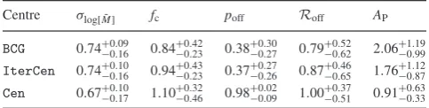
Table 4. Constraints on the halo model parameters using the three defini-tions of halo centre. For each of the parameters, we quote the median of the posterior distribution, marginalized over the other parameters, while the errors are the 16th and 84th percentile of the distribution. All the constraints derived using the three different proxies for the halo centre agree within 1σ.

Centre σ_{log[ ˜M]} fc poff Roff AP

BCG 0.74+₋0₀._.09₁₆ 0.84₋+0₀._.42₂₃ 0.38+₋0_0..₂₇30 0.79+₋0_0..₆₂52 2.06+₋1₀._.19₉₉ IterCen 0.74+₋00..1016 0.94+−00..4323 0.37−+00..2726 0.87−+00..4665 1.76+

1.12

−0.87

Cen 0.67+₋00..1017 1.10+−00..3246 0.98−+00..0209 1.00−+00..3751 0.91+ 0.63

−0.33

84th percentiles of the posterior distribution. We discuss the con-straints on the model parameters in further detail in the remainder of this section.

5.1.1 Masses of dark matter haloes

The dark matter halo masses of the galaxy groups that host the stacked galaxy groups analysed in this work span one and a half orders of magnitude withM∈[1013_{. . . 10}14.5_]h−1_M

. Since our ESD profiles extend to large radii, our 2h−1_{Mpc cut-off is larger}

thanR200over this full mass range, these mass measurements are robust and direct as they do not require any extrapolation. The uncertainties on the masses are obtained after marginalising over the other model parameters. Typically these errors are 15 per cent larger than what would be derived by fitting anNFWprofile to the same data, ignoring the scatter in mass inside each luminosity bins. Note that a simpleNFWfit to the data in the six luminosity bins, with fixed concentration (Duffy et al.2008) would also lead to a bias in the inferred masses of approximately 25 per cent.

The inferred halo masses in each luminosity bin are slightly cor-related due to the assumption that the scatter in halo mass is constant in different bins of total luminosity. We compute the correlation be-tween the inferred halo masses from their posterior distribution, and we show the results in Fig.10. Overall, the correlation is at most 20 per cent, and this is accounted for when deriving scaling relations (see Section 6).

5.1.2 Concentration and mis-centring

The shape of the ESD profile at scales smaller than∼200h−1_kpc

contains information on the concentration of the halo and on the mis-centring of the BCG with respect to the true halo centre. How-ever, the relative normalization of the concentration–halo mass re-lation,fc, and the two mis-centring parameters,poff andRoff are degenerate with each other. A small value offc has a similar ef-fect on the stacked ESD as a large offset: both flatten the profile. To further illustrate this degeneracy, we show in Fig.11the 2D posterior distribution of the average projected offset (poff ×Roff)

Figure 10. Correlation matrix between the mean halo masses derived in the sixr-band luminosity bins from the halo model fit. The reason for the correlation is the assumption of a constant scatter as a function of group luminosity in the halo occupation distribution.

Figure 11. 2D posterior distribution of the average projected offset (poff × Roff) and the normalization of the concentration–halo mass relationfc. The

contours indicate the 68, 95, and 99 per cent confidence region.

and the normalization of the concentration–halo mass relation. It is clear how a vanishing offset would require a low value of the concentration.