Confidence sets for the date of a break in level and trend when the order of integration is unknown

Con…dence Sets for the Date of a Break in Level and Trend when

the Order of Integration is Unknown

David I. Harvey and Stephen J. Leybourne School of Economics, University of Nottingham

June 2014

Abstract

We propose methods for constructing con…dence sets for the timing of a break in level and/or trend that have asymptotically correct coverage for both I(0) and I(1) processes. These are based

on inverting a sequence of tests for the break location, evaluated across all possible break dates. We separately derive locally best invariant tests for the I(0) and I(1) cases; under their respective assumptions, the resulting con…dence sets provide correct asymptotic coverage regardless of the

magnitude of the break. We suggest use of a pre-test procedure to select between the I(0)- and I(1)-based con…dence sets, and Monte Carlo evidence demonstrates that our recommended procedure achieves good …nite sample properties in terms of coverage and length across both I(0) and I(1)

environments. An application using US macroeconomic data is provided which further evinces the value of these procedures.

Keywords: Level break; Trend break; Stationary; Unit root; Locally best invariant test; Con…-dence sets.

JEL Classi…cation: C22.

1

Introduction

It has now been widely established that structural change in the time series properties of

macroeco-nomic and …nancial time series is commonplace (see, inter alia, Stock and Watson (1996)), and much

work has been devoted to this area of research in the literature. Focusing on the underlying trend

func-tion of a series, the primary issues to be resolved when considering the possibility of structural change

are whether a break is present, and, if so, when the break occurred. The focus of this paper concerns

the latter issue regarding the timing of the break, and is therefore complementary to procedures that

focus on break detection. A proper understanding of the likely timing of a break in the trend function

is crucial for modelling and forecasting e¤orts, and is also of clear importance when attempting to

gain economic insight into the cause and impact of a break. While a number of procedures exist to

determine a point estimate of a break in level and/or trend, this paper concentrates on ascertaining

the degree of uncertainty surrounding break date estimation by developing procedures for calculating

a con…dence set for the break date, allowing practitioners to identify a valid set of possible break

points with a speci…ed degree of con…dence.

The methodology of Bai (1994) allows construction of a con…dence set for a break in level in a

time series, extended in Bai (1997) to allow for a break in trend, with the con…dence set comprised

of a con…dence interval surrounding an estimated break point, with the interval derived from the

asymptotic distribution of the break date estimator. However, as Elliott and Müller (2007) [EM]

argue, the asymptotic theory employed in this approach relies on the break magnitude being in some

sense “large”, in that the magnitude can be asymptotically shrinking only at a rate su¢ ciently slow

to permit break detection procedures to have power close to one, so that although the magnitude is

asymptotically vanishing, the break is still large enough to be readily detectable. EM argue that in

many practical applications it is “small” breaks (for which detection is somewhat uncertain) that are

typically encountered, and these authors go on to demonstrate that for smaller magnitude breaks, the

Bai approach results in con…dence sets that su¤er from coverage rates substantially below the nominal

level, with the true break date being excluded from the con…dence set much too frequently. EM

suggest an alternative approach to deriving con…dence sets that achieve asymptotic validity, based on

inverting a sequence of tests of the null that the break occurs at a maintained date, with the resulting

con…dence set comprised of all maintained dates for which the corresponding test did not reject. By

deriving a locally best invariant test that is invariant to the magnitude of the break under the null,

the EM con…dence sets have asymptotically correct coverage, regardless of the magnitude of the break

(and therefore regardless of whether the magnitude is treated as …xed or asymptotically vanishing).

The EM model and assumptions pertain to a break in a linear time series regression, of which a

break in level is a special case. They do not, however, consider the case of a break in linear trend,

hence our …rst contribution is to develop an EM-type methodology for calculating asymptotically valid

con…dence sets for the date of a break in trend (and/or level). As in their approach, we derive a locally

best invariant test of the null that the break occurs at a maintained date, and make an expedient

choice for the probability measure used in deriving the test so as to render the resulting test statistic

asymptotically invariant to the break timing.

When attempting to specify the deterministic component of an economic time series in practice,

a critical consideration is the order of integration of the stochastic element of the process. Given the

prevalence of integrated data, it is important to develop methods that are valid in the presence of

I(1) shocks. Moreover, since there is very often a large degree of uncertainty regarding the order of

integration in any given series, it is extremely useful to have available techniques that are robust to

the order of integration, dealing with the potential for either stationary or unit root behaviour at

the same time as specifying the deterministic component. A body of work has developed in recent

years focusing on such concerns, developing order of integration-robust tests for a linear trend (e.g.

for a break in trend (e.g. Harvey et al. (2009), Perron and Yabu (2009b), Sayg¬nsoy and Vogelsang

(2011)), and tests for multiple breaks in level (e.g. Harvey et al. (2010)). Most recently, Harvey and

Leybourne (2013) have proposed methods for estimating the date of a break in level and trend that

performs well for both I(0) and I(1) shocks.

In the current context, it is clear that reliable speci…cation of con…dence sets for the date of a break

in level/trend will be dependent on the order of integration of the data under consideration. Perron

and Zhu (2005) extend the results of Bai (1994, 1997) to allow for I(1), as well as I(0), processes when

estimating the timing of a break in trend or level and trend, and di¤erent distributional results are

obtained under I(0) and I(1) assumptions. Similarly, and as would be expected, we show that the

EM procedure for calculating con…dence sets, which is appropriate for I(0) shocks, does not result

in sets with asymptotically correct coverage when the driving shocks are actually I(1). However,

extension to the I(1) case is possible via a modi…ed approach applied to the …rst di¤erences of the

data, whereby the level break and trend break are transformed into an outlier and a level break,

respectively. This development comprises the second main contribution of our paper. Since there is

typically uncertainty surrounding the integration order in practice, we propose a unit root

pre-test-based procedure for calculating con…dence sets that are asymptotically valid regardless of the order

of integration of the data. We …nd the new procedure allows construction of con…dence sets with

correct asymptotic coverage under both I(0) and I(1) shocks (irrespective of the magnitude of the

break). We also examine the performance of our procedure under local-to-I(1) shocks, and …nd that it

displays asymptotic over-coverage (i.e. coverage rates above the nominal level), hence the con…dence

sets are asymptotically conservative in such situations, including the true date in the con…dence set

at least as frequently as the nominal rate would suggest. Monte Carlo simulations demonstrate that

our recommended procedure performs well in …nite samples, in terms of both coverage and length (the

number of dates included in the con…dence set as a proportion of the sample size).

The paper is structured as follows. Section 2 sets out the level/trend break model. Section 3 derives

the locally best invariant tests for a break at a maintained date in both the stationary and unit root

environments. The large sample properties under the null of correct break placement are established

when correct and incorrect orders of integration are assumed, with the implications discussed for the

corresponding con…dence sets based on these tests. The properties of feasible variants of these tests,

and corresponding con…dence sets, are subsequently investigated. In section 4 we propose use of a unit

root pre-test to select between I(0) and I(1) con…dence sets when the order of integration is not known.

The …nite sample behaviour of the various procedures is examined in section 5. Here we also consider

trimming as a means of potentially shortening the con…dence sets. Section 6 provides empirical

illustrations of our proposed procedure using US macroeconomic data, while section 7 concludes.

The following notation is also used: ‘_{b c}’denotes the integer part, ‘₎’denotes weak convergence,

2

The model and con…dence sets

We consider the following model which allows for a level and/or a trend break in either a stationary

or unit root process. The DGP for an observed series ytwe assume is given by

yt = 1+ 2t+ 11(t >b 0Tc) + 2(t b 0Tc)1(t >b 0Tc) +"t; t= 1; :::; T (1)

"t = "t 1+ut; t= 2; :::; T; "1=u1 (2)

with _b 0Tc 2 f2; :::; T 2g T the level and/or trend break point with associated break fraction

0. In (1), a level break occurs at time b 0Tc when 1 6= 0; likewise, a trend break occurs if 2 6= 0. The parameters ₁, ₂, 1 and 2 are unknown, as is the break pointb 0Tc, inference on which is the

central focus of our analysis. Our generic speci…cation for"tis given by (2) assuming that 1< 1

and thatutis I(0).

For an assumed break point _b T_{c 2} T, our interest centres on testing whether or not b 0Tc

and _b T_c coincide, which we can write in hypothesis testing terms as a test of the null hypothesis

H0 :b 0Tc =b Tc against the alternative H1 :b 0Tc 6=b Tc. Then, following EM, a (1 )-level

con…dence set for 0 is constructed by inverting a sequence of -level tests of H0 : b 0Tc = b Tc

for _b T_{c 2} T, with the resulting con…dence set comprised of all b Tc for which H0 is not rejected.

Provided the test of H0 :b 0Tc =b Tc has size for all b Tc, the con…dence set will have correct

coverage, since the probability of excluding 0from the con…dence set (via a spurious rejection ofH0) is

. In terms of con…dence set length, a shorter than(1 )-level con…dence set arises whenever the tests

of H0 :b 0Tc=b Tc reject with probability greater than under the alternativeH1 :b 0Tc 6=b Tc

across _b T_c. Other things equal, the more powerful a test is in distinguishing between H0 and H1,

the shorter this con…dence set should be. Note that this approach to constructing con…dence sets does

not guarantee that the set is comprised of contiguous sample dates, cf. EM (p. 1207).

In the next section, we consider construction of powerful tests of H0 against H1, deriving locally

best invariant tests along the lines of EM when = 0and when = 1, under a Gaussianity assumption

forut. The large sample properties of these tests are subsequently established under weaker conditions

for and ut.

3

Locally best invariant tests

For the purposes of constructing locally best invariant tests, we make the standard assumption that

ut N IID(0; 2u), and we suppose that in (2) is restricted to taking the two values = 0 or = 1.

In the case of = 0, we …nd that (1) reduces to

yt= 1+ 2t+ 11(t >b 0Tc) + 2(t b 0Tc)1(t >b 0Tc) +ut; t= 1; :::; T (3)

while for = 1, (1) can be written as

Now write either of the models (3) or (4), for an arbitrary break point _b T_c, in the generic form

zt=d0t +d0;t +ut (5)

where = [ 1 2]0, and, under (3), zt=yt,dt= [1t]0, = [ 1 2]0,d ;t= [1(t >b Tc) (t b Tc)1(t >

b T_c)]0; while under (4), zt = yt, dt = 1, = 2, d ;t = [1(t = b Tc+ 1) 1(t > b Tc)]0. In an

obvious matrix form, (5) can be expressed as

z=D +D +u: (6)

We consider tests based onu^, the vector of OLS residuals from the regression (6), that is,u^=M z,

where M =I C (C0C ) 1C with C = [D:D ]. Such tests are by construction invariant to the

unknown parameters and under H0. The likelihood ratio statistic for testingH0 against H1 can

then be derived as follows. Let k and T denote the number of regressors and the e¤ective sample

size, respectively, in the regression (6). Also, let B be the T (T k ) matrix de…ned such that

B0_{B =IT k and B B}0 _{=M . SinceB}0_z=B0_{u^ is invariant to , it follows that, on setting = 0}

without loss of generality, B0z N(B0D 0 ;

2

uIT k ) under H1. Under H0, B0z = B0₀z is also invariant to , hence, on setting = = 0 without loss of generality, B0z N(0; 2_uIT k ). The

likelihood ratio statistic is then

LR( ; ; 0) =

(2 2_u) (T k )=2exp_f (2 2_u) 1(B0z B0D 0 )0(B0z B0D 0 )g

(2 2

u) (T k )=2expf (2 u2) 1(B0z)0B0zg

= exp[ (2 2_u) 1_f(B0z B0D 0 )0(B0z B0D 0 ) (B0z)0B0zg]

= exp_{f u}2z0B B0D 0

1 2

2

u 0D00B B

0_D

0 g

= exp( _u2u^0D 0

1 2

2

u 0D00M D 0 ):

Following the approach of Andrews and Ploberger (1994), to remove the dependence of the statistic

on the parameters and 0, we consider tests that maximize the weighted average power criterion

X

b Tc2 T; b Tc6=b Tc

b Tc

Z

P(test rejects_{j b} 0Tc=b Tc; = )dvb Tc( )

over all tests that satisfyP(test rejects_{j b} 0Tc=b Tc) = , where the weightsf tg are non-negative

real numbers and_fvt( )gis a sequence of non-negative measures onR2. This yields a test of the form

LR( ) = X

b Tc2 T; b Tc6=b Tc

b Tc

Z

LR( ; f; )dv_{b Tc}(f):

As in EM, we set _b Tc= 1, such that equal weights are placed on alternative break dates, and take

v_b Tc(f) to be a probability measure of N(0; b2Hb Tc). We then obtain (after some algebra)

LR( ) = X

b Tc2 T; b Tc6=b Tc

I+b2 _u2H_b TcD0M D

1=2

Taking a …rst order Taylor series expansion of LR( ) in the locality of b2 = 0, we …nd that the

stochastic component of LR( ), up to a constant of proportionality, is given by

S( ) = X

b Tc2 T; b Tc6=b Tc

^

u0D H_{b Tc}D0u:^ (7)

This represents the locally best invariant test with respect to b2 that maximizes weighted average

power, for givenH_{b Tc}.

We specify H_b Tc separately under the models (3) and (4), and, as in EM, we construct the

elements of H_{b Tc} using particular scalings of _b T_c and (T _b T_c) such that the resulting S( )

tests have asymptotic distributions under H0 that do not depend on . This choice is justi…ed by

the convenience of allowing the same asymptotic critical value to apply to each of the sequence of

individual tests over _b T_{c 2} T. Given these choices for H_b Tc, explicit forms for (7) can be derived

under both (3) with = 0 and (4) with = 1, as detailed in the following lemma.

Lemma 1

(a) Under DGP (3) ( = 0), when

H_{b Tc}=

8 > > > > > < > > > > > :

"

b T_c 2 0

0 _b T_c 4

#

if _b T_c<_b T_c

"

(T _b T_c) 2 0

0 (T _b T_c) 4

#

if _b T_c>_b T_c

(8)

it follows from (7) that, for testing H0 against H1, the locally best invariant test with respect to b2 is

given by

S0( ) = b Tc 2 b_XTc 1

t=2

t

X

s=1

^

us

!2

+_b T_c 4

b_XTc 1

t=2

t

X

s=1

(s t)^us

!2

(9)

+(T _b T_c) 2

T_X2

t=b Tc+1

0 @

t

X

s=b Tc+1

^

us

1 A

2

+ (T _b T_c) 4

T_X2

t=b Tc+1

0 @

t

X

s=b Tc+1

(s t)^us

1 A

2

where _fu^_tgT

t=1 denote the residuals from OLS estimation of (3) whenb 0Tc is replaced by b Tc.

(b) Under DGP (4) ( = 1), when

H_b Tc=

8 > > > > > < > > > > > :

"

b T_c 1 0

0 _b T_c 2

#

if _b T_c<_b T_c

"

(T _b T_c) 1 ₀

0 (T _b T_c) 2

#

if _b T_c>_b T_c

it follows from (7) that, for testing H0 against H1, the locally best invariant test with respect to b2 is

given by

S1( ) = b Tc 1 b_XTc 1

t=2

^

u2_t+1+_b T_c 2

b_XTc 1

t=2

t

X

s=2

^

us

!2

(11)

+(T _b T_c) 1

T_X2

t=b Tc+1

^

u2_t+1+ (T _b T_c) 2

T_X2

t=b Tc+1

0 @

t

X

s=b Tc+1

^

us

1 A

2

where _fu^_tgT

t=2 denote the residuals from OLS estimation of (4) whenb 0Tc is replaced by b Tc.

3.1 Large sample properties of the test procedures

Now we have the structures of the tests in place, we can derive their large sample properties under

more general assumptions regarding and ut. Here we make one of the two following assumptions:

Assumption I(0) Let _{j j} < 1, ut = C(L) t; C(L) =

P₁

i=0CiLi; C0 = 1, with C(z) 6= 0 for all jz_j 1 and P1_i=0i_jCij<1, and where tis an IIDsequence with mean zero, variance 2 and …nite

fourth moment.

Under Assumption I(0) we de…ne the long-run variance of ut as !2u = limT!1T 1E(PTt=1ut)2 = 2_C(1)2_{. Note that the long-run variance of"}

t is then given by!2" =!2u=(1 )2.

Assumption I(1) Let = 1with ut de…ned as in Assumption I(0).

Under Assumption I(1) we also de…ne the short-run variance ofutas 2u =E(u2t). The theorem below

gives the null limiting distributions of the e¢ cient testsS0( )and S1( )under Assumptions I(0) and

I(1), respectively.

Theorem 1

(a) Under H0 :b 0Tc=b Tc and Assumption I(0),

!_"2S0( ))

Z 1

0

B2(r)2dr+

Z 1

0

K(r)2dr+

Z 1

0

B0₂(r)2dr+

Z 1

0

K0(r)2dr _L0:

(b) Under H0 :b 0Tc=b Tc and Assumption I(1),

!_u2_fS1( ) 2 2ug )

Z 1

0

B1(r)2dr+

Z 1

0

B₁0(r)2dr _L1

where

B1(r) = B(r) rB(1);

B2(r) = B(r) rB(1) + 6r(1 r)

1 2B(1)

Z 1

0

B(s)ds ;

K(r) = r2(1 r)B(1)

Z r

0

B(s)ds+r2(3 2r)

Z 1

0

with B(r) a standard Brownian motion process, and where B₁0(r), B₂0(r)and K0(r) take the same

forms as B1(r), B2(r) and K(r), respectively, but withB(r) replaced byB0(r), with B0(r) a standard

Brownian motion process independent of B(r). (Note that B1(r), B2(r) and K(r) are tied down and

Bj(r) is a j’th level Brownian bridge.)

Remark 1 Note that, as desired, !_"2S0( ) and !u2fS1( ) 2 2ug have nuisance-parameter free

distributions that do not depend on . This property arises from the speci…c functions for H_b T_c

adopted, justifying the H_{b Tc} choices made in Lemma 1. Note also that the_L1 distribution coincides

with the null limit distribution of the test proposed by EM in the case of a single regressor that is

subject to a break.

Remark 2 The result in Theorem 1 (b) is obtained because both the …rst and third terms ofS1( )in

(11) converge in probability to 2_u. These components ofS1( )are associated with testing on the

one-time dummy variable in (4), and it can easily be shown that these terms also converge in probability

to 2_u under the alternativeH1 when only a level break occurs under Assumption I(1), i.e. when an

outlier of magnitude 1 is present in the I(0) …rst di¤erences of the series. As such, S1( ) does not

have asymptotic power for identifying the date of a break in level in I(1) data. This is to be expected

given that an unscaled level break is asymptotically irrelevant in an I(1) series. However, retaining

these terms in the statistic (11), along with a judicious choice of 2_u estimator (discussed below), can

yield …nite sample performance bene…ts, hence we do not omit these terms from the S1( )statistic.

Remark 3 A theoretical alternative to our approach would be to attempt to endow the …rst

and third terms of S1( ) with a null limit distribution rather than a probability limit. However,

this would require a rescaled and centered variant of the form _b T_c 1=2Pb_t=2Tc 1(^u2_t+1 2_u) for

the …rst component (and similarly for the third component). This introduces two complications;

…rst, 2_u is unknown and ultimately needs replacing with an estimator, which we generically

de-note ~2_u. Since ~2_u is at best Op(T 1=2)-consistent for 2u, it follows that the asymptotic

distribu-tion of _b T_c 1=2Pb_t=2Tc 1(^u2_t+1 ~2_u) will be di¤erent to that of _b T_c 1=2P_tb₌₂Tc 1(^u2_t+1 2_u). Sec-ondly, even if 2

u is known, b Tc 1=2

Pb Tc 1

t=2 (^u2t+1 2u) implicitly involves the partial sum process

T 1=2P_tb₌₁rTc(u2_t 2_u), while the third term ofS1( )involves the partial sum processT 1=2Pb_t=1rTcut;

the joint limit distribution of these two partial sum processes depends on the third moment of ut,

which is also unknown. As a result, we adopt the more analytically tractable speci…cation outlined in

Lemma 1 (b).

Table 1 gives simulated (upper tail) -level critical values for the limit distributions _L0 and L1.

These were obtained by direct simulation of the limiting distributions given in Theorem 1,

approx-imating the Brownian motion processes using N IID(0;1) random variates, and with the integrals

approximated by normalized sums of 2000 steps. The simulations were programmed in Gauss 9.0

tests!_"2S0( )under Assumption I(0), and!u2fS1( ) 2 2ugunder Assumption I(1), the

correspond-ing con…dence set based on invertcorrespond-ing these tests will have asymptotically correct coverage of (1 ),

regardless of the magnitude of the break in level and/or trend.

We next consider the behaviour of S0( ) and S1( ) under H0 when an incorrect assumption

regarding the value of is made.

Theorem 2

(a) Under H0 :b 0Tc=b Tc and Assumption I(1),

!_"2S0( ) =Op(T2):

(b) Under H0 :b 0Tc=b Tc and Assumption I(0),

!_u2_fS1( ) 2 2ug=!u22fE( "t)2 2ug+Op(T 1=2):

Theorem 1 (a) shows that a (nominal)(1 )-level con…dence set based on!_"2S0( )will be

asymptot-ically empty (i.e. zero coverage) as all the test statistics diverge to+₁and thereby exceed the -level

critical value in the limit. Theorem 1 (b) shows that!_u2_fS1( ) 2 2ug converges in probability to a

constant that takes the value!_u22_fE( "t)2 2ug. If this constant exceeds the -level critical value,

then the con…dence set based on!_u2_fS1( ) 2 2ug will also be asymptotically empty (zero coverage);

if it is less than the -level critical value, then the con…dence set based on !_u2_fS1( ) 2 2ug will

be asymptotically full (i.e. coverage of unity). Which of these two cases pertains will depend on the

values of!2_u,E( "t)2and 2u. Trivially, a su¢ cient condition for the latter case isE( "t)2 2u, since

then !_u2_fS1( ) 2 2ug assumes a negative probability limit, which can never exceed the (positive)

asymptotic critical value. Clearly then, an incorrect assumption regarding the order of integration of

"tnegates the validity of con…dence sets based on inverting sequences of these e¢ cient tests, an issue

we revisit in section 4.

The tests considered so far are clearly infeasible since they depend on the unknown parameters

!2

", or!2u and 2u. In the next section we examine some feasible versions of the tests and reassess the

content of Theorems 1 and 2 in the context of these.

3.2 Feasible test procedures and their large sample properties

To make the tests feasible, we require suitable estimators of !2_" for S0( ) and !2u and 2u forS1( ).

To estimate the long-run variances !2_" and !2_u we consider both non-parametric and parametric

ap-proaches. In the non-parametric case, we employ the Bartlett kernel-based estimators

^

!2_{i;N P}( ) = ^_i;0( ) + 2

`N P

X

l=1

h(l; `N P)^i;l( ); ^i;l( ) =T 1 T

X

t=l+1

^

utu^t l

for i = _f"; u_g, where the u^t are the residuals obtained from OLS estimation of regression (3) when

i="and (4) when i=u.1 Here, h(l; `N P) = 1 l=(`N P + 1), with a lag truncation parameter `N P

that is assumed to satisfy the standard condition that, as T _{! 1},1=`N P +`3N P=T !0.

1_{For economy of notation we do not discriminate between the di¤erent numbers ofu^}

In the parametric case, we employ Berk-type autoregressive spectral density estimators which can

be written as

^

!2_i;P( ) = s

2 i

^2_i

where ^i is obtained from the …tted OLS regression

^

ut= ^ ^ut 1+

`P

X

l=1

^

j u^t l+ ^et; t=`P + 1; :::; T

and s2

i =T 1

PT

t=`P+1^e

2

t. Again, the u^t are obtained from (3) if i=", and from (4) if i=u. Also,

`P is assumed to have the same properties as`N P above.

It is also natural to consider estimating 2_u with ^2_u( ) = ^_u;0( ) using the u^t from (4). The

following lemma gives the large sample behaviour of the various estimators.

Lemma 2

(a) Under H0 :b 0Tc=b Tc and Assumption I(0),

^

!2_{";N P}( ); !^2_";P( ) _!p !2_";

^

!2_{u;N P}( ) = Op(`_{N P}1 );

^

!2_u;P( ) = Op(`_P2);

^2_u( ) = E( "t)2+Op(T 1=2):

(b) Under H0 :b 0Tc=b Tc and Assumption I(1),

^

!2_{";N P}( ) = Op(`N PT);

^

!2_";P( ) = Op(T2);

^

!2_{u;N P}( ); !^2_u;P( ) _!p !2_u;

^2_u( ) _!p 2_u:

The results for !^2_{";N P}( ), !^2_{u;N P}( ) and ^2_u( ) arise from a simple adaptation of results shown in

Harveyet al. (2009); those for!^2_";P( )and !^2_u;P( ) arise similarly from Harveyet al. (2010).

We can now de…ne feasible versions of the statistics as

^

S_0;j( ) = !^_";j2( )S0( );

^

S_1;j( ) = !^_u;j2( )_fS1( ) 2^2u( )g

forj=_fN P; P_g. Based on Theorem 1 and Lemma 2, we then have the following corollary.

Corollary 1

(a) Under H0:b 0Tc=b Tcand Assumption I(0),

^

(b) Under H0:b 0Tc=b Tc and Assumption I(1),

^

S_{1;N P}( ),S^_1;P( )_{) L}1:

These results simply show that when a correct order of integration is assumed (and therefore the

appropriate limit critical values are employed), con…dence sets based on the feasible tests will continue

to provide asymptotically correct coverage. From Theorem 2 and Lemma 2 we have the following

corollary.

Corollary 2

(a) Under H0:b 0Tc=b Tcand Assumption I(1),

^

S_{0;N P}( ) = Op(`N P1 T) p ! 1; ^

S_0;P( ) = Op(1):

(b) Under H0:b 0Tc=b Tc and Assumption I(0),

^

S_{1;N P}( ) = Op(`N PT 1=2) p !0;

^

S_1;P( ) = Op(`2PT 1=2)

8 > > < > > :

p

!0 `P =o(T1=4)

=Op(1) `P =O(T1=4) p

! 1 `_P1 =o(T1=4₎

:

Corollary 2 (a) shows that a (nominal)(1 )-level con…dence set based onS^_{0;N P}( )will be

asymptot-ically empty, thereby paralleling the behaviour of its infeasible counterpart. However, the behaviour

of a con…dence set based on S^_0;P( ) is uncertain since it is an Op(1) variate (whose behaviour will

actually depend on !2_u). It is, however, almost certain to be the case that this con…dence set will

have incorrect coverage asymptotically. From Corollary 2 (b), a con…dence set based on S^_{1;N P}( )

will be asymptotically full. All possibilities - unit, incorrect (dependent on!2_") or zero coverage - can

arise with S^_1;P( ), contingent on how`P is chosen. The results of Corollary 2 therefore reinforce the

importance of assuming a correct order of integration, since use of an incorrect assumption results in

a procedure with asymptotic coverage di¤erent from(1 ).

We should be aware that the properties of!^2_i;j( )and ^2_u( )shown in Lemma 2 - particularly their

consistency properties, will not hold in general underH1 :b 0Tc 6=b Tc (the exception being when

a level break alone occurs under Assumption I(1)). In view of this, we might entertain employing

alternate estimators of !^2_i;j( ) and ^2_u( ) based on some estimator of 0. Below we will consider

the break fraction estimator derived in Harvey and Leybourne (2013), therein referred to as ^Dm.

This estimator is the value of that yields the minimum sum of squared residuals from an OLS

regression of y = [y1; y2 y1; :::; yT yT 1]0 on Z ; = [z1;z2 z1; :::;zT zT 1]0 where zt =

[1; t;1(t > _b T_c);(t _b T_c)1(t > _b T_c)]0 across _b T_{c 2} T and across 2 Dm. In what follows

we set T = fb0:01Tc; :::;b0:99Tcg and, following Harvey and Leybourne (2013), we set Dm =

f0;0:2;0:4;0:6;0:8;0:9;0:95;0:975;1_g. It can be shown that !^2_i;j(^Dm) and ^

2

asymptotic properties as those for!^2_i;j( )and ^2_u( )shown in Lemma 2, and also that these properties

will continue to hold underH1. This gives rise to the potential for power improvements underH1, and

therefore potentially narrower con…dence sets. In what follows we therefore also consider versions of

theS^_i;j( )procedures where!^2_i;j( )and ^2_u( )are replaced with!^2_i;j(^Dm)and ^

2

u(^Dm), respectively,

i.e.

^

S₀^_;j( ) = !^_";j2(^Dm)S0( );

^

S₁^_;j( ) = !^_u;j2(^Dm)fS1( ) 2^

2

u(^Dm)g:

4

Selecting between I(0)- and I(1)-based con…dence sets

Given the foregoing discussions, it should be clear that we want to base con…dence set construction

on theS^k_0;j( )(j=_fN P; P_g,k=_f ;^_g) suite of test statistics under Assumption I(0) and theS^₁k_;j( )

statistics under Assumption I(1). One way or another, in practice this has to involve deciding whether

a given data set is more compatible with Assumption I(0) or Assumption I(1) and then applying ^

S₀k_;j( )orS^₁k_;j( )as appropriate. The most direct way of doing this is to apply a unit root test in the

role of a pre-test. To this end, we employ the in…mum GLS-detrended Dickey-Fuller test of Perron

and Rodríguez (2003) and Harveyet al. (2013). In the current context, this statistic is calculated as

MDF = inf

b Tc2 _T

DFGLS_c ( )

where _T = [_b lTc;b UTc] with l and U representing trimming parameters. Here DFGLSc ( )

denotes the standard t-ratio associated with ~ in the …tted ADF-type regression

~

ut= ~ ~ut 1+

`DF

X

j=1

~

j u~t j+ ~et; t=k+ 2; :::; T;

with`DF having the same properties as `N P above, and

~

ut=yt ~1 ~2t ~11(t >b Tc) ~2(t b Tc)1(t >b Tc)

where[~₁;~₂;~1;~2]0 is obtained from a local GLS regression of y onZ ; with = 1 +c=T.

The limiting distribution of the MDF statistic under the null hypothesis of Assumption I(1) when

1 = 2 = 0 is given by the expression in equation (11) of Perron and Rodríguez (2003) on setting

c = 0. Let cv denote an asymptotic -level (left-tail) critical value from this distribution. Our

pre-test-based decision rule is then to select S^₀k_;j( )if MDF < cv and select S^₁k_;j( )if MDF cv .

Under Assumption I(0), MDF diverges to ₁ at the rate Op(T1=2) so that S^k0;j( ) is selected with

probability one in the limit; this occurs regardless of whether 1 and 2 are zero or non-zero. Under

Assumption I(1), S^₁k_;j( ) is selected with limit probability 1 when 2 = 0, irrespective of the

magnitude of 1. When 2 6= 0 (and again irrespective of 1), the asymptotic size of MDF is only

slightly below , so that S^₁k_;j( ) is selected with limit probability a little above 1 . In order to

^

S₀k_;j( )with probability one in the limit under Assumption I(0), the MDF pre-test can be conducted

at a signi…cance level that shrinks with the sample size, by replacing cv with cv ;T, where cv ;T

satis…es cv ;T ! 1and cv ;T =o(T1=2), i.e. a critical value that diverges to 1 at a rate slower

thanT1=2_.

In what follows, we denote our pre-test-based tests of H0 :b 0Tc=b Tc as follows:

^

S_pre;jk ( ) =

(

^

S₀k_;j( ) ifMDF < cv ;T

^

S₁k_;j( ) ifMDF cv ;T

; j=_fN P; P_g; k=_f ;^_g:

In the limit, it follows that underH0:b 0Tc=b Tc,

^

S_pre;jk ( )₎

(

L0 under Assumption I(0) L1 under Assumption I(1)

; j =_fN P; P_g; k =_f ;^_g

and so comparison of S^k

pre;j( ) with critical values from L0 if MDF < cv ;T or from L1 if MDF

< cv ;T, will lead to correctly sized tests asymptotically. Inference based on the inversion of sequences

of such tests o¤ers the possibility of reliable con…dence set construction without the need to make an

a priori (and possibly incorrect) assumption regarding the order of integration. Given the uncertainty

surrounding the unit root properties of typical economic and …nancial series, particularly those that

are subject to a break in level/trend, such an approach has obvious appeal.

Thus far we have considered the cases _{j j}<1 and = 1 to evaluate the behaviour of the di¤erent

procedures under stationary and unit root assumptions. It is also important to assess the behaviour

of S^k_pre;j( ) under a local-to-unity speci…cation for . Adopting the usual Pitman drift speci…cation

= 1 +cT 1, c 0, MDF is an Op(1) variate, and hence, due to the fact that cv ;T ! 1,

^

S_pre;jk ( ) = ^S₁k_;j( ) in the limit. It can then be easily shown (along the lines of the proof of Theorem

1) that, forc 0 underH0,

^

S_pre;jk ( )_{) L}c₁( ); j=_fN P; P_g; k =_f ;^_g

where

Lc1( ) = 2

Z

0

n

Bc(r)

r

Bc( )

o2

dr+ (1 ) 2

Z 1

Bc(r) Bc( )

r

1 (Bc(1) Bc( ))

2

dr

(12)

with Bc(r) =

Rr

0e

(r s)c_{dB(s). Note that on setting c= 0 we obtain} L01( )

d

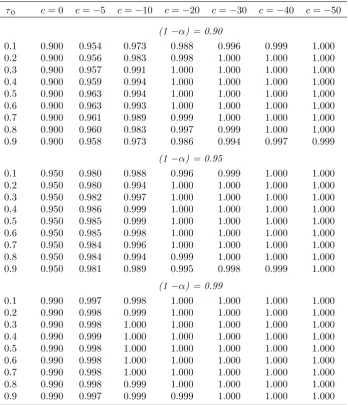
=_L1 8 . Table 2 reports

asymptotic coverage rates for nominal 0.90-, 0.95- and 0.99-level con…dence sets constructed from the ^

S_pre;jk ( ) tests, using critical values from Table 1 (which are appropriate for c = 0). The coverage

rates were obtained by direct simulation of (12) in the same manner as the simulations for Table 1,

and results are reported for c = _f0; 5; 10; 20; 30; 40; 50_g and 0 = f0:1;0:2; :::;0:9g, noting

that the _Lc₁( 0) distribution depends on 0 unlessc= 0. It is clear from the results that in the

local-to-unity setting, con…dence sets based on the S^_pre;jk ( ) tests do not su¤er from any under-coverage

acrossc or 0; indeed, over-coverage is observed, increasing in cfor a given 0. This arises from the

values appropriate for a pure unit root are being applied, and translates to conservative con…dence

sets that asymptotically include the true break date with a probability at least as great as the nominal

coverage rate. This reassuring property indicates that asymptotic under-coverage is not a feature of

our proposed pre-test-based con…dence sets for any value of , be it unity, local-to-unity, or strictly

less than one.

Finally, an alternative feasible approach to constructing a con…dence set with correct asymptotic

coverage under both Assumption I(0) and Assumption I(1) (and with over-coverage under a

local-to-unity speci…cation) is to consider taking a union of an I(0)-based con…dence set and an I(1)-based

con…dence set. Given the results of Corollary 2, it is evident that asymptotically correct coverage, i.e.

a coverage rate of(1 ) in both the I(0) and I(1) cases, would be obtained only from a union of the

con…dence sets corresponding toS^₀k_{;N P}( )andS^₁k_;P( ), with the latter requiring we set`_P1 =o(T1=4).

All other unions would lead to either asymptotically full coverage (i.e. a coverage rate of one), or

a coverage rate that depends on nuisance parameters (!2_u or !2_"). We investigated the …nite sample

properties of such a union, and while the coverage rates were found to be comparable to those of the

best of the pre-test procedures, the union con…dence set lengths were generally greater than those

a¤orded by the best pre-test approach (in some cases substantially so), hence we do not pursue the

union further here.

In the next section we evaluate the …nite sample properties of our pre-test-based approaches in

comparison with those that are based on a maintained assumption regarding the integration properties

of the data, both in terms of coverage and length.

5

Finite sample performance

In this section we examine the …nite sample performance of con…dence sets based on theS^₀k_;j( ),S^₁k_;j( )

andS^_pre;jk ( )tests (j=_fN P; P_g,k=_f ;^_g). We simulate the DGP (1)-(2) with ₁ = ₂ = 0(without

loss of generality) and a range of break magnitudes, 1 and 2, and timings, 0, for the sample sizes

T = 150andT = 300. We consider _{2 f}0:00;0:50;0:80;0:90;0:95;1:00_gto encompass both I(1) and a

range of I(0) DGPs, and setut N IID(0;1). TheS^0k;j( )andS^1k;j( )tests are applied at the nominal

0.05-level using the asymptotic critical values provided in Table 1, with`N P =`max= 12(T =100)1=4

and `P selected via the Bayesian information criterion with maximum value `max. For the S^_pre;jk ( )

tests, we select between S^₀k_;j( ) and S^k_1;j( ) on the basis of MDF conducted at the 0.05-level with

c= 17:6(following Harveyet al. (2013)), l= 1 U = 0:01,2and where`DF is selected according to

the MAIC procedure of Ng and Perron (2001), as modi…ed by Perron and Qu (2007), with maximum

lag order `max. All simulations were conducted using 10,000 Monte Carlo replications, and in the

tables we report results for con…dence set coverage (the proportion of replications for which the true

break date is contained in the con…dence set) and con…dence set length (in each replication, length is

2

From simulation of the asymptotic null distribution ofMDFin this case, we …nd thatcv0:05= 3:88. For simplcity,

calculated as the number of dates included in the con…dence set as a proportion of the sample size;

we then report the average length over Monte Carlo replications).

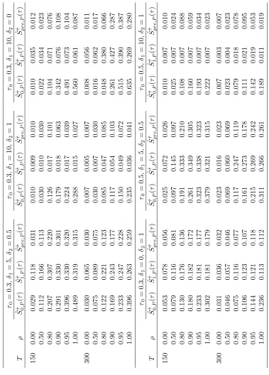
Table 3 reports results for 0 = 0:3, 1 = 5 and 2 = 0:5, such that both a level and trend break

occur before the sample mid-point. Consider …rst the behaviour of the con…dence sets based onS^k

0;j( )

(j =_fN P; P_g, k= _f ;^_g). When = 0, we …nd that (approximately) correct coverage is achieved

for the two S^₀k_;P( ) sets, whereas the two S^₀k_{;N P}( ) sets display correct coverage only for T = 300,

with under-coverage apparent for T = 150. When = 1, theS^₀k_{;N P}( )sets deliver substantial

under-coverage, increasingly so in the larger sample size, as our asymptotic results in Corollary 2 suggest.

In contrast, the S^k

0;P( ) sets (the tests for which were found to beOp(1)), display over-coverage for

both sample sizes, which is clearly less of a concern. For = 0:5, the coverage rates for the S^₀k_;j( )

sets are seen to be broadly similar to those for = 0, then as increases towards one, coverage moves

closer to those observed in the = 1 case, as we might expect in …nite samples.

Turning now to the S^₁k_;j( ) sets, all are seen to provide (approximately) correct coverage when

= 1, in line with our theoretical results; indeed, coverage never deviates from 0.95 by more than

0.01 across both sample sizes. At the other extreme, when = 0 we …nd that all the S^₁k_;j( ) sets

show under-coverage for both T = 150and T = 300(which is somewhat surprising in the case of the

two S^₁k_{;N P}( ) sets, since the tests converge in probability to zero under Assumption I(0), although

unreported simulations con…rm that coverage does start to increase for larger samples); under-coverage

is also seen in some cases when = 0:5, while for the larger values of <1, coverage is closer to the

correct coverage seen when = 1 (in fact some over-coverage is displayed in these cases).

For our proposed pre-test-based procedures S^k

pre;j( ), we see that in each case, coverage is very

close to the corresponding S^₁k_;j( ) coverage for = 1 and values close to 1, but then for small

values of assumes the more accurate coverage rates of the corresponding S^k

0;j( ) sets. Of course,

the coverage of any given S^_pre;jk ( ) set is limited by the coverage performance of the corresponding

underlying S^₀k_;j( ) and S^₁k_;j( )sets, thus for the two S^_{pre;N P}k ( ) sets, under-coverage is still manifest

for some settings, due to the under-coverage inherent in the S^₀k_{;N P}( ) sets. However, the S^_pre;Pk ( )

sets show good …nite sample coverage rates across the range of settings considered in the table, in

particular avoiding problems of under-coverage.

When considering our results for the length of the con…dence sets implied by the di¤erent tests,

as we would expect, length generally decreases (since test power generally increases) as T increases

and as decreases. Comparing the di¤erent procedures, the most striking feature is that any given ^

S_i;j^ ( ) orS^_pre;j^ ( )set (where the short and long run variance estimators used in the tests are based

on ^Dm) substantially outperforms the corresponding S^i;j( ) or S^pre;j( ) set (where the estimators

in the tests are evaluated at each ). This is entirely to be expected, since under the alternative

hypothesis, use of a consistent estimator of the true break fraction allows consistent estimation of 2 u

and !2_u under Assumption I(1) and consistent estimation of !2_" under Assumption I(0). In contrast,

the estimators ^2_u( ), !^2_u( ) and !^2_"( ) are not consistent when ₆= 0, and are likely to over-state

the values of the true parameters, thereby reducing the values of the test statistics and increasing

^

S_{pre;N P}^ ( )andS^₁^_;P( )were found to su¤er from problems of under-coverage, making them unreliable

on that measure. Overall, then, it is clear that the two procedures that can be deemed in some sense

satisfactory, on both coverage and length grounds, areS^₀^_;P( )andS^_pre;P^ ( ). Of these two procedures, ^

S^

pre;P( )su¤ers from less over-coverage, and also has arguably the best length properties across the

range of values considered; speci…cally, S^_pre;P^ ( ) and S^₀^_;P( ) have similar length for = 0, 0:5,

0:8 and 0:95, and while S^_pre;P^ ( ) has somewhat greater length than S^₀^_;P( ) for = 0:9, it o¤ers a

more marked improvement in length when = 1, as we would expect given the ability of S^_pre;P^ ( )

to select the better-performingS^₁^_;P( )set in this scenario. It is also reassuring to see that for values

of less than but close to one, the preferred S^^

pre;P( ) procedure has decent length properties. For

these large values of < 1, the local-to-unity asymptotic results are potentially relevant, and it is

clear that despite theS^_pre;P^ ( )procedure being conservative in such cases (displaying over-coverage),

the procedure retains an ability to achieve a reasonably short length, demonstrating that while the

underlying tests may be under-sized for local-to-unity processes, they still have power to reject for

incorrect break dates.

Table 4 reports results for the same settings as Table 3, except with a larger magnitude level

and trend break, with 1 = 10 and 2 = 1. As regards coverage, much the same comments apply

as for Table 3.3 As we would expect, the lengths of the con…dence sets are generally smaller in this

case of larger, more detectable, breaks. Once more, we …nd that S^_pre;P^ ( ) is the best performing

procedure overall; indeed, compared to the only other procedure with reliable coverage and decent

length,S^₀^_;P( ), we see thatS^_pre;P^ ( )now displays equal or shorter length across all values of , with

decreases in length of up to 0.28 seen.

Table 5 reports results for the case of 1 = 10 and 2 = 0 so that only a level break occurs.

Consider …rst the results for = 1. From Remark 1, it follows that here the S^k

1;j( )tests have zero

asymptotic power to identify the date of the level break; this can be seen in the table as the lengths

of all the S^₁k_;j( ) sets increase between T = 150 and T = 300. What we observe, however, is that,

for a given T, the sets based on S^₁^_;j( ) are very much shorter than those based onS^_1;j( ).4 Taking

the results across the di¤erent values of together, we again …nd S^_pre;P^ ( ) to be the best procedure

when considering both coverage and length, with the gains in length over S^^

0;P( ) when = 1 now

even more marked than was observed in Tables 3 and 4.

In Table 6 we have 1 = 0 and 2 = 1 so that only a trend break is present. Here we …nd the

3_{Note that the coverage rates for the S^}

i;j( ) sets are numerically identical across di¤erent 1 and 2 settings, since

they are invariant to these parameters by construction underH0.

4_{This arises because there is an upward bias in ^}2

u( ) relative to ^2u(^Dm) resulting from the former being based on residuals from a regression containing a mis-speci…ed break component whenever ₆= 0, while the latter uses an

estimator of 0 which, albeit not consistent, can nonetheless perform reasonably in …nite samples. This relative upward

bias translates to lower values ofS^1;j( )compared toS^1^;j( ), negatively a¤ecting the power of the former and the length

of the corresponding con…dence set. Indeed, the lengths of theS^1;j( )sets are close to the nominal coverage rates, and

similar to what would be obtained if the …rst and third terms ofS1( ) (and consequently the2^2u( ) centering) were

simply omitted from the statistic, unlikeS^1^;j( )where inclusion of the …rst and third terms ofS1( )(together with the

2^2

pattern of results mimic those of Table 4, albeit with lengths tending to be somewhat greater due to

the lack of contribution of a level break. What is clear from all these results is that S^^

pre;P( ) is the

preferred test for construction of con…dence sets.

Tables 7 and 8 report results for the same settings as Tables 3 and 4, respectively (i.e. cases

where both a level and trend break occur), but with the breaks occurring at the sample mid-point, i.e.

0 = 0:5, rather than 0 = 0:3. Comparing the coverage results across 0= 0:3and 0= 0:5, while the under-coverage associated with the S^₀k_{;N P}( ) sets for = 1is exaggerated for a mid-point break, the

most noticeable feature is that the under-coverage seen for theS^₁k_;j( )sets for the smaller values of is

here replaced byover-coverage. This ensues partly because when = 0 = 0:5, it can easily be shown

that the di¤erence between the sum of the …rst and third components of S1( ) in (11) and 2^2u( )

(or2^2_u(^Dm)) isop(T

1=2_{), as opposed to when =}

0 6= 0:5where this di¤erence is only Op(T 1=2)

and tends to be positive. Other things equal, therefore, when = 0 = 0:5the chance of the S^1k;j( )

test rejecting in …nite samples is reduced relative to when = 0 6= 0:5. However, despite S^1k;j( )

performing relatively well for these mid-point breaks, one could not rely on this approach to deliver

reliable con…dence sets in general, given the absence of knowledge regarding 0 and the possibility of

under-coverage for non-central breaks. Taking the results of Tables 7 and 8 as a whole, it is still the

case thatS^_pre;P^ ( )performs very well.

Unreported results for the case of 0 = 0:7 also con…rm that S^pre;P^ ( ) is the best performing

procedure overall. Therefore, our recommendation would clearly be for theS^_pre;P^ ( )procedure, given

its reliable …nite sample coverage and good performance in terms of con…dence set length.

5.1 Con…dence sets based on trimming

An issue that may be relevant in …nite samples is that when is close to zero the …rst two components

ofS0( )in (9) and S1( )in (11) are based on only a few of theu^t residuals; similarly, when is close

to one the same is true of the last two components of S0( )and S1( ). Therefore, it is possible that

for values of near the(0;1)extremities, the …nite sample behaviour of the tests may di¤er markedly

from the behaviour of the same tests evaluated at less extreme values of . In our above simulations,

coverages were calculated for = 0 = 0:3 and 0:5 - values well away from the extremities, so no

such problems should arise there. That said, there is clearly a potential for values ofS^_i;jk ( )calculated

near the extremities of to adversely in‡uence the lengths of the resulting con…dence sets (these

being potentially non-contiguous). To investigate this, we recalculated the lengths of the sets based

onS^₀^_;P( ),S^₁^_;P( )and our preferred testS^_pre;P^ ( )only for_b T_{c 2} 0_T =_fb0:1T_c; :::;_b0:9T_cg, which

can be thought of as a 10% trimming, akin to the assumption that no break can occur in the …rst

and last 10% of the observed data, an assertion frequently made in the associated structural change

literature.

The results are shown in Table 9. The …rst block of results in Table 9 is for 0 = 0:3, 1 = 5 and

length reductions of up to about 0:13.5 This implies that, in some cases, a signi…cant proportion of

non-rejections of H0 are incorrectly occurring for tests being evaluated at the extreme values of ,

since 0 itself is not close to these extremes. When T = 300, the length reduction is up to about

0:07 so that, for this speci…cation, trimming is less e¤ective with the larger sample size, implying

that the untrimmed con…dence sets contain relatively few anomalous extreme dates. The second

block of results is for 0 = 0:3, 1 = 10 and 2 = 1, i.e. where the break magnitudes are doubled.

Comparing with Table 4 we …nd that, for both T = 150 and T = 300, there appears to be very

little (if any) reduction in length arising from trimming, again implying, for this speci…cation, few

spurious rejections ofH0 occur for tests evaluated at extreme values of . In the third block of Table

9 where 0 = 0:3, 1 = 10 and 2 = 0, we see, on comparing with Table 5, that trimming is again

e¤ective, and more so for T = 300than forT = 150. For the remaining speci…cations in Table 9 (the

lower blocks), comparison with Tables 6-8 shows generally only very modest shortenings arising from

trimming. Overall, however, we conclude that trimming can be of possible bene…t in improving the

length of con…dence sets, potentially removing spurious dates from the set that have arisen purely due

to the sampling variability involved in the tests when evaluated near the extremes.

6

Empirical illustrations

As empirical illustrations of our con…dence set procedures for dating a break in level and/or trend,

we apply them to two US macroeconomic series. These are the nominal money supply M2 (seasonally

adjusted, measured in logarithms) and the e¤ective federal funds rate, using monthly data over the

period 1959:1-2012:12 (T = 648). The data were obtained from the FRED database of the Federal

Reserve Bank of St Louis. We construct 0.95-level con…dence sets employing the three procedures ^

S^

0;P( ), S^1^;P( ) and S^pre;P^ ( ) (note the con…dence set for S^pre;P^ ( ) is either that for S^0^;P( ) or

^

S₁^_;P( ), depending on the outcome of MDF), using the same settings as were applied in the Monte

Carlo simulations above.

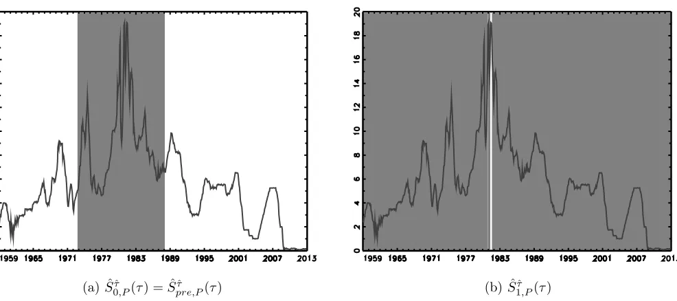
Results for the M2 series are shown in Figure 1, where the con…dence sets are represented by the

shaded regions, while the series overlays the sets. Figure 1 (a) reports the con…dence set for S^₀^_;P( )

which is contiguous here with a length of 0.51 (330 observations) covering the interval 1971:4-1998:9.

In Figure 1 (b), we see that the con…dence set for S^₁^_;P( ) is much shorter, with length 0.33 (213

observations), but is not contiguous. In particular, the set is comprised of an almost contiguous

subset of dates covering the interval 1978:6-1994:2 (the dates 1986:10-1987:2 inclusive are exceptions

to this), plus a number of dates towards the extremes of the sample, the latter lying within 0:03T of

the sample’s beginning and end. If we view the end-point behaviour as spurious and apply a trimming

rule of at least 3%, cf. section 5.1, we e¤ectively ignore the non-rejections associated with these very

early and very late dates. The resulting con…dence set then contains the almost contiguous subset

of dates alone, with the length of the set reducing to 0.28. Visual inspection of the plot of the M2

series con…rms that a break in this date range is plausible. The con…dence set selected by our pre-test

5

procedureS^_pre;P^ ( )is that ofS^₁^_;P( ), and hence the shorter and more plausible of the two, reinforcing

the case for using such an approach in practice.

Figure 2 gives the results for the federal funds rate series. Here S^₀^_;P( ) yields a contiguous

con…dence set with length0:28 (181 observations) covering the interval 1972:12-1987:12, which again

appears consistent with the visual plot of the data. The con…dence set associated with S^₁^_;P( ) has

length 0.98, which is rather meaningless as a con…dence set for a break since it includes nearly all

observations in the sample. Our pre-test procedureS^_pre;P^ ( )selects the con…dence setS^₀^_;P( ), which

is without any doubt the more plausible of the two. These examples taken together highlight the

potential shortcomings of simply constructing con…dence sets based onS^^

0;P( )orS^1^;P( )alone, while

simultaneously demonstrating the bene…ts of the S^_pre;P^ ( ) approach.

7

Conclusions

In this paper we have proposed methods for constructing con…dence sets for the timing of a break

in level and/or trend that have asymptotically correct coverage regardless of the order of integration

(and are asymptotically conservative in the case of local-to-unity processes). Our approach follows

the work of EM, and is based on inverting a sequence of tests for the break location, evaluated across

the full spectrum of possible break dates. We propose two locally best invariant tests upon which

the con…dence sets can be based, each of which corresponds to a particular order of integration (i.e.

I(0) or I(1) data generating processes). Under their respective assumptions, these con…dence sets

provide correct asymptotic coverage regardless of the magnitude of the break in level/trend, and

also display good …nite sample properties in terms of both coverage and length. When the tests

are applied under an incorrect assumption regarding the order of integration, they perform relatively

poorly, however. Consequently, we propose use of a pre-test procedure to select between the

I(0)-and I(1)-based con…dence sets. Monte Carlo evidence shows that our recommended pre-test based

procedure works well across both I(0) and I(1) environments, o¤ering practitioners a reliable and

robust approach to constructing con…dence sets without the need to make an a priori assumption

concerning the data’s integration order. Application to two US macroeconomic series provides further

evidence as to the e¢ cacy of these procedures.

References

Andrews, D. and Ploberger, W. (1994). Optimal tests when a nuisance parameter is present only

under the alternative. Econometrica 62, 1383-1414.

Bai, J. (1994). Least squares estimation of a shift in linear process. Journal of Time Series Analysis

15, 453-472.

Bai, J. (1997). Estimation of a change point in multiple regression models. Review of Economics

Bunzel, H. and Vogelsang, T.J. (2005). Powerful trend function tests that are robust to strong serial

correlation, with an application to the Prebisch-Singer hypothesis. Journal of Business and

Economic Statistics 23, 381-394.

Elliott, G. and Müller, U.K. (2007). Con…dence sets for the date of a single break in linear time

series regressions. Journal of Econometrics 141, 1196-1218.

Harvey, D.I. and Leybourne, S.J. (2013). Break date estimation for models with deterministic

struc-tural change. Oxford Bulletin of Economics and Statistics, in press.

Harvey, D.I., Leybourne, S.J. and Taylor, A.M.R. (2007). A simple, robust and powerful test of the

trend hypothesis. Journal of Econometrics 141, 1302-1330.

Harvey, D.I., Leybourne, S.J. and Taylor, A.M.R. (2009). Simple, robust and powerful tests of the

breaking trend hypothesis. Econometric Theory 25, 995-1029.

Harvey, D.I., Leybourne, S.J. and Taylor, A.M.R. (2010). Robust methods for detecting multiple

level breaks in autocorrelated time series. Journal of Econometrics 157, 342-358.

Harvey, D.I., Leybourne, S.J. and Taylor, A.M.R. (2013). Testing for unit roots in the possible

pres-ence of multiple trend breaks using minimum Dickey-Fuller statistics. Journal of Econometrics,

177, 265-284.

Ng, S. and Perron, P. (2001). Lag length selection and the construction of unit root tests with good

size and power. Econometrica 69, 1519-1554.

Perron, P. and Qu, Z. (2007). A simple modi…cation to improve the …nite sample properties of Ng

and Perron’s unit root tests. Economics Letters 94, 12-19.

Perron, P. and Rodríguez, G. (2003). GLS detrending, e¢ cient unit root tests and structural change.

Journal of Econometrics 115, 1-27.

Perron, P. and Yabu, T. (2009a). Estimating deterministic trends with an integrated or stationary

noise component. Journal of Econometrics 151, 56-69.

Perron, P. and Yabu, T. (2009b). Testing for shifts in trend with an integrated or stationary noise

component. Journal of Business and Economic Statistics 27, 369-396.

Perron, P. and Zhu, X. (2005). Structural breaks with deterministic and stochastic trends. Journal

of Econometrics 129, 65-119.

Sayg¬nsoy, Ö. and Vogelsang, T.J. (2011). Testing for a shift in trend at an unknown date: a …xed-b

analysis of heteroskedasticity autocorrelation robust OLS based tests. Econometric Theory 27,

Stock, J.H. and Watson, M.W. (1996). Evidence on structural instability in macroeconomic time

series relations. Journal of Business and Economic Statistics 14, 11-30.

Vogelsang, T.J. (1998). Testing for a shift in mean without having to estimate serial-correlation

parameters. Journal of Business and Economic Statistics 16, 73-80.

Appendix

Proof of Lemma 1

(a) To show (9), note that

D0u^=

" _PT

t=b Tc+1u^t

PT

t=b Tc+1(t b Tc)^ut

#

: (13)

Also, since we have the orthogonality conditionD0u^= 0,

" _PT

t=b Tc+1u^t

PT

t=b Tc+1(t b Tc)^ut

#

=

"

0

0

#

and from the orthogonality conditionD0_{u^= 0,}

" PT

t=1u^t

PT

t=1tu^t

#

=

"

0

0

#

:

So, for_b T_c<_b T_c, (13) can be written as

D0u^=

" _{Pb Tc}

t=1 u^t

Pb Tc

t=1 (t b Tc)^ut

#

:

For_b T_c>_b T_c,

T

X

t=b Tc+1

^

ut =

T

X

t=b Tc+1

^

ut

b_XTc

t=b Tc+1

^

ut

=

b_XTc

t=b Tc+1

^

ut

T

X

t=b Tc+1

(t _b T_c)^ut = T

X

t=b Tc+1

(t _b T_c)^ut

b_XTc

t=b Tc+1

(t _b T_c)^ut

=

T

X

t=b Tc+1

(t _b T_c)^ut+ (b Tc b Tc) T

X

t=b Tc+1

^

ut

b_XTc

t=b Tc+1

(t _b T_c)^ut

=

b_XTc

t=b Tc+1

such that (13) can be written as

D0u^=

2 4

Pb Tc

t=b Tc+1u^t

Pb Tc

t=b Tc+1(t b Tc)^ut

3 5:

Using (8), it follows that

S( ) =

b_XTc 1

b Tc=2

8 < :b Tc

2

0 @

b_XTc

t=1

^

ut

1 A

2

+_b T_c 4

0 @

b_XTc

t=1

(t _b T_c)^ut

1 A

29

= ;

+

T_X2

b Tc=b Tc+1

8 <

:(T b Tc)

2

0 @

b_XTc

t=b Tc+1

^

ut

1 A

2

+ (T _b T_c) 4

0 @

b_XTc

t=b Tc+1

(t _b T_c)^ut

1 A

29

= ;

= _b T_c 2

b_XTc 1

t=2

t

X

s=1

^

us

!2

+_b T_c 4

b_XTc 1

t=2

t

X

s=1

(s t)^us

!2

+(T _b T_c) 2

T_X2

t=b Tc+1

0 @

t

X

s=b Tc+1

^

us

1 A

2

+ (T _b T_c) 4

T_X2

t=b Tc+1

0 @

t

X

s=b Tc+1

(s t)^us

1 A

2

= S0( ):

(b) To show (11), paralleling the proof of Lemma 1(a), we …nd

D0u^ =

"

^

u_b Tc+1

PT

t=b Tc+1u^t

#

=

8 > > > > > < > > > > > :

"

^

u_{b Tc+1}

Pb Tc

t=2 u^t

#

for _b T_c<_b T_c

"

^

u_{b Tc+1}

Pb Tc

t=b Tc+1u^t

#

for _b T_c>_b T_c :

Then, using (10),

S( ) =

b_XTc 1

b Tc=2

8 < :b Tc

1_u^2

b Tc+1+b Tc 2

0 @

b_XTc

t=2

^

ut

1 A

29

= ;

+

T_X2

b Tc=b Tc+1

8 <

:(T b Tc)

1_u^2

b Tc+1+ (T b Tc) 2

0 @

b_XTc

t=b Tc+1

^

ut

1 A

29

= ;

= _b T_c 1

b_XTc 1

t=2

^

u2_t+1+_b T_c 2

b_XTc 1

t=2

t

X

s=2

^

us

!2

+(T _b T_c) 1

T_X2

t=b Tc+1

^

u2_t+1+ (T _b T_c) 2

T_X2

t=b Tc+1

0 @

t

X

s=b Tc+1

^

us

1 A

2

Proof of Theorem 1

In what follows we may set ₁ = ₂ = 0 and 1= 2 = 0 without loss of generality.

(a) Let W(r) = !"B(r). In view of S0( ), the limits we require are those of (i) T 1=2Pbt=1rTcu^t for

t _b T_c, (ii) T 1=2P_tb₌rT_bc_Tc+1u^t fort > b Tc and (iii) T 3=2Pb_t=1rTc(t brTc)^ut fort b Tc, (iv)

T 3=2Pb_t=rT_bc_Tc+1(t _brT_c)^utfor t >b Tc. To show (i) write

T 1=2

b_XrTc

t=1

^

ut = T 1=2

b_XrTc

t=1

0

@ut b Tc 1 b_XTc

s=1

us

1 A

0 B @

T 3=2Pb_s=1Tcus s b Tc 1Pbj=1Tcj

T 3Pb Tc

s=1 s b Tc

1Pb Tc

j=1 j

2

1 C AT 2

b_XrTc

t=1

0

@t _b T_c 1

b_XTc

s=1

s

1 A

= T 1=2

b_XrTc

t=1

ut brTc b Tc 1T 1=2

b_XTc

s=1

us

0 B @T

3=2Pb Tc

s=1 sus b Tc 1T 1Pbj=1TcjT 1=2

Pb Tc

s=1 us

T 3Pb Tc

s=1 s b Tc

1Pb Tc

j=1 j

2

1 C A

0 @T 2

b_XrTc

t=1

t _brT_{c b} T_c 1T 2

b_XTc

s=1

s

1 A

) W(r) rW( )

R

0 sdW(s)

2

2 W( )

3

12

!

r2

2

r 2

2

= W(r) rW( ) +6r( ₃ r)

2W( )

Z

0

W(s)ds

and for (ii),

T 1=2

brT_c

X

t=b Tc+1

^

ut = T 1=2

brT_c

X

t=b Tc+1

0

@ut (T b Tc) 1 T

X

s=b Tc+1

us

1 A

0 B @

T 3=2PT_{s=b Tc+1}us s (T b Tc) 1PTj=b Tc+1j

T 3PT

s=b Tc+1 s (T b Tc) 1

PT

j=b Tc+1j

2

1 C A

T 2

b_XrTc

t=b Tc+1

0

@t (T _b T_c) 1

T

X

s=b Tc+1

s