A fast and explicit algorithm for simulating the dynamics of small dust
grains with smoothed particle hydrodynamics
Daniel J. Price
1‹and Guillaume Laibe
2‹1Monash Centre for Astrophysics and School of Physics & Astronomy, Monash University, Clayton, VIC 3800, Australia 2School of Physics and Astronomy, University of St. Andrews, North Haugh, St. Andrews, Fife KY16 9SS, UK
Accepted 2015 May 1. Received 2015 April 24; in original form 2015 March 13
A B S T R A C T
We describe a simple method for simulating the dynamics of small grains in a dusty gas, relevant to micron-sized grains in the interstellar medium and grains of centimetre size and smaller in protoplanetary discs. The method involves solving one extra diffusion equation for the dust fraction in addition to the usual equations of hydrodynamics. This ‘diffusion approximation for dust’ is valid when the dust stopping time is smaller than the computational timestep. We present a numerical implementation using smoothed particle hydrodynamics that is conservative, accurate and fast. It does not require any implicit timestepping and can be straightforwardly ported into existing 3D codes.
Key words: hydrodynamics – methods: numerical – protoplanetary discs – dust, extinction –
ISM: kinematics and dynamics.
1 I N T R O D U C T I O N
Small grains rule the interstellar medium (ISM). Micron-sized dust grains absorb ultraviolet radiation from hot, young stars and re-emit it in the infrared. Understanding how these grains interact with the gas is critical to understanding both the dynamics and thermody-namics of the ISM, and to interpreting observational results which usually assume a fixed gas-to-dust ratio in order to derive physical quantities such as the gas column density.
Modelling such grains presents a severe computational challenge, since small grains are tightly coupled to the gas by the mutual drag force. This presents both a short time-scale problem, since the stopping time of the grains is much shorter than the typical computational time, and a short length-scale problem, since the physical separation between the dust grain population and the gas is much smaller than typical distances in the ISM.
In a recent series of papers (Laibe & Price2012a,b,2014a,b,c), we have outlined the limitations associated with modelling dust and gas using the standard two-fluid approach, where they are regarded as separate fluids coupled by a drag term. Typically, the gas is represented by a set of particles or grid cells, while the dust is represented by a separate set of pressure-less particles coupled to the gas by a drag term. The length and time-scale problems discussed above mean that with this approach one needs both infinite spatial and temporal resolution to accurately capture the dynamics of small grains in the limit of perfect coupling (Laibe & Price2012a; but see
E-mail: [email protected] (DJP); [email protected] (GL)
Lor´en-Aguilar & Bate2014for an alternative approach). However, this is the limit in which the mixture can be accurately described as a single fluid moving at the barycentric velocity. In Laibe & Price (2014a,b, hereafterLP14a,b), we showed how the equations for a coupled dust–gas system can be reformulated to describe this single-fluid mixture without loss of generality, solving both the length and time-scale issues and also preventing artificial trapping of dust particles below the resolution of the gas (Ayliffe et al.2012; Laibe & Price2012a, hereafterLP12a). The method is similar to the approach to other multi-fluid systems in astrophysics such as ionized plasmas (Pandey & Wardle2008), but more general since it can be implemented without any approximations.
InLP14b, we derived a smoothed particle hydrodynamics (SPH) algorithm based on the fully general one-fluid method and showed that it could accurately capture the dynamics of dust–gas mixtures in both the weakly coupled and tightly coupled limits. For problems involving small grains, however, the full machinery of the one-fluid formulation is unnecessary and a much simpler and computation-ally inexpensive approach is possible, as outlined in Section 3.3 of
LP14a. This approximation is accurate when the stopping time,ts, is less than the Courant timestep (equation 115 inLP14a).
Our goal in this paper is to derive a numerical implementation of this much simpler formulation, since there are many situations in astrophysics where the dynamics of small grains is the dominant effect. This includes simulations of galaxies, star formation in the ISM – where small grains control the thermodynamics – and the settling and migration of dust in protoplanetary discs. We summa-rize the analytic formulation and its applicability in Section 2, the numerical implementation is described in Section 3 and tests are presented in Section 4. A public version of theNDSPMHDcode (v2.1)
2015 The Authors
at University of St Andrews on August 13, 2015
http://mnras.oxfordjournals.org/
implementing the algorithms and with the precise setup of the test problems is released alongside this paper.1
2 T H E D I F F U S I O N A P P R OX I M AT I O N F O R D U S T
2.1 Continuum equations
2.1.1 General case
In LP14a we showed that, to first order ints/T, whereT is the time-scale for a sound wave to propagate over a typical distanceL, the equations describing the evolution of a dust–gas mixture can be written in the form
dρ
dt = −ρ(∇ ·v), (1)
dv
dt =(1−)fg+fd+ f, (2) d
dt = − 1
ρ∇ ·[(1−)ρtsf], (3)
du dt = −
P ρg
(∇ ·v)−ts(f · ∇)u+heat−cool, (4)
whereρ is the total density of the mixture,≡ρd/ρis the mass fraction of dust, f represents accelerations acting on both compo-nents of the fluid while fgand fdrepresent the accelerations acting on the gas and dust components, respectively,f ≡ fd− fgis the differential acceleration between the gas and dust,uis the specific thermal energy of the gas,Pis the gas pressure, andheatandcool are additional heating and cooling terms, respectively.2The velocity vis the barycentric velocity of the mixture, defined as
v≡ ρdvd+ρgvg
ρ =vd+(1−)vg. (5)
In the so-calledterminal velocity approximation(Youdin & Good-man2005; Chiang2008; Barranco2009; Lee et al.2010; Jacquet, Balbus & Latter2011) assumed in equations (1)–(4),f is rapidly balanced by the drag. Thus, the time dependence of the differential velocity can be ignored, and the differential velocity between the gas and dust is given by
v≡(vd−vg)tsf. (6)
This also implies that the anisotropic pressure term in the mo-mentum equation (seeLP14a) should be neglected. The terminal velocity approximation is valid when the drag coefficientKis large such that the stopping time,
ts≡
ρdρg
K(ρd+ρg)
= (1−)ρ
K , (7)
is short compared to the timestep. Various physical prescriptions forKin the Epstein and Stokes drag regimes are given in Laibe & Price (2012b, hereafterLP12b) but the essential point is thatKis inversely proportional to the grain size, being large for small grains.
1http://users.monash.edu.au/∼dprice/ndspmhd/
2Equation (4) differs from the expression we gave for the ‘first-order approx-imation’ inLP14a. The drag heating term,v2/ts, is clearly negligible in the terminal velocity approximation and thePdVwork term should involve ∇ ·vrather than∇ ·vg. Both approximations are required for the numer-ical scheme to conserve total energy as defined in the terminal velocity approximation (equation 39).
The differential accelerationf depends on the physics in the problem, i.e. the forces affecting the gas but not the dust, which may include pressure, magnetic and other forces. In our numerical implementation, we consider the contributions from the pressure gradient (see below) and also the artificial viscosity term, which should likewise affect the gas only.
2.1.2 Hydrodynamics
For the simple case of hydrodynamics, the only force is the pressure gradient, giving
fg= − ∇P
ρg ; fd=0, (8)
and thus
f = ∇P
ρg , (9)
giving equations (1)–(4) in the form dρ
dt = −ρ(∇ ·v), (10)
dv dt = −
∇P
ρ + f, (11)
d dt = −
1
ρ∇ ·(ts∇P), (12)
du dt = −
P ρg
(∇ ·v)−ts
ρg
(∇P· ∇u)+heat−cool. (13)
These are similar to the usual equations of hydrodynamics in the absence of dust. The only differences are the extra equation that describes the evolution of the dust fraction, the modifications to the thermal energy equation and the fact that the pressure is related to thegasdensity only, not the total density (see Section 2.1.3 below; this gives the zeroth-order effect of a ‘heavy fluid’, as discussed in
LP14a).
2.1.3 Equation of state
The equation set is closed by the usual equation of state specifying the gas pressureP in terms of the gas density and temperature. Unless otherwise specified in this paper, we assume an adiabatic equation of state, i.e.
P =(γ−1)ρgu=(γ−1)(1−)ρu, (14)
whereγis the usual adiabatic constant.
2.2 Timestepping
The main change when adopting the formulation given above com-pared to hydrodynamics is the addition of the diffusion equation for the dust fraction (12). This introduces an additional constraint on the timestep when the diffusion coefficient is large. Assuming an isothermal equation of stateP =c2
sρg=c2s(1−)ρand a constant density, equation (12) can be written as a simple diffusion equation for:
d
dt = ∇ ·(η∇), (15)
where the diffusion coefficientη≡tsc2s. This implies a stability constraint of the form
t < t=C0
h2
η =C0
h2
tscs2
, (16)
at University of St Andrews on August 13, 2015
http://mnras.oxfordjournals.org/
whereC0is a dimensionless safety factor of order unity andhis the resolution length (the smoothing length in SPH). We can rewrite equation (16) as
t < C
tCour
ts
2
ts, (17)
whereCis a constant andtCour =C0h/csis the usual Courant condition. This implies that the timestep is constrained when the stopping time islong– the opposite of the usual situation where the timestep is constrained when the stopping time is short. This is the main advantage of using the diffusion approximation – small grains can be integrated explicitly.
Specifically, the diffusion timestep becomes the limiting timestep when
ts> tCour. (18)
However, this is also the criterion for when the terminal veloc-ity approximation breaks down (seeLP14a). This implies that the diffusion approximation becomes inaccurate precisely when the timestep implied by equation (16) starts to constrain the timestep, because at this point the time dependence inv becomes im-portant. Once this occurs, one should revert to the general for-mulation given byLP14b where v is explicitly evolved, or a two-fluid method. Physically this transition occurs once grains grow beyond a certain size, implying that the stopping time be-comes long, or equivalently when one has enough temporal resolu-tion to resolve the time-scale on which the differential velocity is changing.
2.3 Validity of the diffusion approximation for astrophysics
Under what circumstances is the diffusion approximation valid for astrophysics? Consider a drag force described by the linear Epstein regime, appropriate to small grains at low Mach number. In this case, the drag coefficient is given by (e.g.LP12b)
K=ρgρd 4π
3
s2 grain
mgrain
8
πγcs, (19)
wheresgrainis the grain size andmgrainis the mass of an individual grain. Assumingmgrain= 43πρgrains3grain, whereρgrainis the intrinsic grain density, the stopping time is
ts=
ρgrainsgrain
ρcs
πγ
8 . (20)
2.3.1 Grains in the ISM
Evaluating this for dust grains in a molecular cloud, we have
ts=2.5×10³yr
ρgrain 1g cm−3
sgrain 0.1μm
ρ
10−20g cm−3
−1
×
cs 0.2 km s−1
−1
. (21)
This indicates that the diffusion approximation is valid for small grains in the ISM, since the stopping time is much smaller than the dynamical time (∼106yr).
2.3.2 Protoplanetary discs
For a protoplanetary disc, the relevant comparison is to the orbital time-scale since the pressure time-scaleH/cs≡1/ . A reasonable criterion for validity is therefore that
ts ≈
ρgrainsgrain
1. (22)
This suggests that the approximation is valid for grain sizes
sgrain102cm
102g cm−2
ρgrain 1 g cm−3
−1
. (23)
Hence, diffusion is a reasonable approximation for grains of∼cm size and smaller in protoplanetary discs. This maximum size is smaller in the outer disc regions, since typically the surface density is inversely proportional to distance from the central star. We examine this experimentally in Section 4.4.
3 I M P L E M E N TAT I O N I N S P H
3.1 Implementation using two first derivatives
The SPH representation of a more general form of equations (1)–(4) has been derived inLP14band so our first approach is to adopt the same discretization but withvprescribed by equation (6), giving
ρa =
b
mbWab(ha), (24)
dva dt = −
b
mb
Pa+qab,aAV aρa2 ∇a
Wab(ha)+Pb+q AV
ab,b bρb2 ∇a
Wab(hb)
+ fa, (25)
da dt = −
b
mb a(1−a)ts,a
aρa fa· ∇aWab(ha)
+ b(1−b)ts,b
bρb fb· ∇aWab(hb)
, (26)
dua dt =
1
a(1−a)ρ2
a
b
mb(Pa+qab,aAV) (va−vb)· ∇aWab(ha)
−ats,a aρa
fa· b
mb(ua−ub)∇aWab(ha), (27)
whereWabis the usual SPH kernel (we use the usual cubic spline
kernel throughout this paper unless otherwise indicated),his the smoothing length, is the usual term related to smoothing length gradients
a≡1−∂ha
∂ρa
b
mb∂Wab(ha)
∂ha ,
(28)
and his related to ρ in the usual manner requiring an iterative procedure to solve equation (24) (Price & Monaghan2004,2007; LP14b) and unless otherwise specified we use a ratio ofhto particle spacing of 1.2 (Price2012). The reader will notice that the first two equations are identical to the usual density summation and momentum equation in SPH. The only differences, mirroring the continuum case (equations 10–13), are the addition of the diffusion equation (26) for the dust fraction, the extra terms in the thermal energy equation (27) and the dependence of the pressure on the gas density rather than the total density in the equation of state (14).
at University of St Andrews on August 13, 2015
http://mnras.oxfordjournals.org/
The differential force between the fluids implied by our formu-lation of equation (25) is
fa= −fag, (29)
where
(1−a)fag= −
b
mb
Pa+qab,aAV aρa2 ∇a
Wab(ha)
+Pb+q AV
ab,b bρb2 ∇a
Wab(hb)
. (30)
Thisf, computed as above, is then used to evaluate equations (26) and (27), requiring a separate loop over the particles.
3.2 Shock-capturing terms
3.2.1 Artificial viscosity
We formulate the artificial viscosity term following the more gen-eral algorithm derived inLP14bbut slightly modified to appear as separateqaandqbterms to avoid averaging the kernel gradients,
following the formulation of artificial viscosity used in thePHANTOM code (Lodato & Price2010; Price & Federrath2010). We use
qAV ab,a= ⎧ ⎨ ⎩− 1
2ρa(1−a)vsig,avab·ˆrab. vab·ˆrab<0
0 vab·ˆrab≥0,
(31)
wherevab≡va−vb(similarly forrab) and the signal speedvsig corresponds to the usual choice for hydrodynamics, i.e.
vsig,a=αacs,a+β|vab·rab|, (32)
whereα∈[0, 1] is the linear dimensionless viscosity parameter [in general this can be individual to each particle, e.g. when using the Morris & Monaghan (1997) or Cullen & Dehnen (2010) switches] andβ(typicallyβ=2) is the von Neumann–Richtmyer viscosity parameter.
The qAV term and the signal speed involve the jump in total velocity rather than the gas velocity, unlike inLP14bwhere only the gas velocity is used. This is both physical and practical. In the terminal velocity approximation, the difference
v−vg≡tsf (33)
is small by definition. The practical side is that we do not knowf prior to the evaluation of equation (25), so it is not possible to use the gas velocity directly in the artificial viscosity term without an iterative approach.
3.2.2 Artificial conductivity
We write the artificial conductivity term, necessary for correct treatment of contact discontinuities (Price 2008), similar to that inLP14b, giving
dua
dt
cond = 1
1−a
b
mb Qab,a aρa2
Fab(ha)+ Qab,b bρb2
Fab(hb)
,
(34)
where∇aWab≡Fabrˆaband
Qab,a= 1
2αuρavsig,u(ua−ub), (35)
with αu ∈ [0, 1] the dimensionless conductivity parameter and
vsig,u= |vab·rˆab|(Price2008; Wadsley, Veeravalli & Couchman
2008).
3.3 Conservation properties
Equation (24) manifestly conserves the total mass since the mass of the SPH particles is constant. Similarly, it can be straightforwardly verified that the total momentum is conserved, since
d dt
a
mava=
a
madva
dt =0, (36)
due to the fact that the resulting double summation is antisymmetric in the particle indicesaandb. Likewise the total angular momentum is conserved, since
d dt
a
mara×va=
a
mara×dva
dt =0 (37)
(for more details, see equation 33 in Price2012). Finally, one may also verify that the total mass of each species is conserved, since
dMd dt = −
dMg dt =
a
ma da
dt =0. (38)
The proof is identical to that given inLP14band again results from the fact that the double summation is antisymmetric with respect to the particle indices.
The total energy of the mixture in the terminal velocity approxi-mation is given by (LP14a)
E= 1
2ρv 2+ρ
gu
dV =
1 2ρv
2+ρ (1−)u
dV . (39)
This is simpler than the full one-fluid expression (equation 61 in
LP14a) as the term involvingv2can be neglected. Discretized on to the mixture particles, the energy becomes
E=
a
ma 1
2v 2
a+(1−a)ua
. (40)
Conservation of energy implies that
dE dt =
a
ma va·dva
dt +(1−a) dua
dt −ua da
dt
=0. (41)
Substituting equations (25) and (26) in the above, we require for energy conservation that
a
ma(1−a)dua dt =
a
b
mamb
Pa+qab,aAV aρa2 va· ∇a
Wab(ha)
+
a
b
mamb
Pb+qab,bAV bρb2 va· ∇a
Wab(hb)
−
a
b
mamb ua(1−a)ats,a
aρa fa· ∇aWab(ha)
−
a
b
mamb ua(1−b)bts,b
bρb fb· ∇aWab(hb)
.
Swapping the summation indices a and b in the second and fourth terms, using the antisymmetry of the kernel gradient
at University of St Andrews on August 13, 2015
http://mnras.oxfordjournals.org/
∇bWba(ha)= −∇aWab(ha) and collecting terms, we have
a
ma(1−a)dua dt
=
a
b
mamb
Pa+qAVab,a aρa2
(va−vb)· ∇aWab(ha)
−
a
b
mamb (1−a)ats,a
aρa (ua−ub)fa· ∇aWab(ha)
,
(42)
from which it is straightforward to verify that, with dua/dtgiven by equation (27), the total energy is conserved exactly.
Thus, the approximate version of the one-fluid algorithm retains all of the conservation properties of both the original SPH method and the general one-fluid approach derived inLP14b.
3.4 Implementation using direct second derivatives
The main disadvantage of the formulation given above is that it requires a third loop over the particles to compute the d/dtterm, beyond the two loops required for the density and force, respectively. This is becausef is required before equation (26) can be eval-uated, but must be computed after the right-hand side of equation (25) is known. Thus, in general this scheme is 1/3 more expensive than a standard SPH code. Here we provide an alternative scheme that does not require this extra loop. The two implementations are compared in Section 4.
3.4.1 Diffusion equation for the dust fraction
We can avoid the extra loop over the particles by discretizing the second derivative in equation (3) directly, similar to the usual way that dissipative terms are treated in SPH. To do this, we assume that viscous forces do not significantly drive the differential velocity between the fluids, i.e. thatfis given by equation (9) and therefore that equation (3) is given by equation (12). We then discretize equation (12) in the usual manner following Cleary & Monaghan (1999):
da dt = −
b
mb
ρaρb(Da+Db) (Pa−Pb)
Fab
|rab|, (43)
whereD ≡ ts, Fab≡ 12[Fab(ha)+Fab(hb)] and Fab is defined
such that∇Wab≡Fabˆrab. It is straightforward to show that this expression also conserves both the total mass of dust and gas, since the resulting double summation in equation (38) is antisymmetric with respect to the particle index.
3.4.2 Harmonic versus arithmetic mean
In the original Cleary & Monaghan (1999) paper (see also Monaghan2005), it was suggested to use the harmonic mean instead of the arithmetic mean of the diffusion coefficient, i.e.
da dt = −
b
mb
ρaρb
4DaDb
(Da+Db)(Pa−Pb)
Fab
|rab|, (44)
with the motivation being that this better handles the case where the diffusion coefficientDis discontinuous. However, we found that this could give incorrect results. Imagine the dust confined to a layer such thata=0 for some particle,a, outside the layer, with
b=0 for particles inside the layer. In this case, the harmonic mean is zero for every pair involving particleasince da/dtisalways
zero. Thus, it is impossible for the layer to move into the region wherewas initially zero, which is clearly incorrect (consider for example a discrete layer of dust descending under gravity). With the arithmetic mean we find no such problem and it is easy to prove that the formulation is correct,3for example with a procedure similar to the one we use in Appendix A.
3.4.3 Thermal energy equation
In order to conserve energy, the corresponding expression for du/dt
when using equation (43) for d/dtis given by dua
dt = 1
a(1−a)ρa2
b
mb(Pa+qab,aAV) (va−vb)· ∇aWab(ha)
+ 1
2(1−a)ρa
b
mb
ρb(ua−ub)(Da+Db)(Pa−Pb)
Fab
|rab|. (45)
At first sight, the second term is a rather strange one and it is not at all clear that this should translate to the correct physical term in equation (27). Yet, amazingly, it does – the proof is given in Appendix A. Hence, there is no disadvantage in using this alternative formulation with respect to conservation properties. The shock-capturing terms remain the same as in Section 3.2.
3.4.4 Choice of smoothing kernel
Although the formulation of second derivatives in SPH using the kernel gradient (43) is now more than 30 years old (Brookshaw
1985), and while it is clearly better than using∇2Wdirectly, to our knowledge there has been no systematic investigation of the best kernel to use in order to compute a second derivative. In particular, on the dust settling test in Section 4.4 we found that using equation (43) with the cubic spline could give quite noisy results. Hence, for this test we instead adopted theM6quintic kernel instead (see Section 4.4). While this results in a more accurate estimate, it is also more expensive due to the larger kernel radius. Hence, a more systematic investigation of suitable kernels for second derivatives in SPH would be valuable here. For example, inLP12awe found double-hump-shaped kernels to be an order of magnitude more accurate compared to standard kernels for computing the drag terms in the two-fluid method at no additional cost.
3.4.5 Two first derivatives versus direct second derivatives
To our knowledge there exists no systematic study on whether it is better to compute second derivatives in SPH directly or using two consecutive first derivatives (though see Watkins et al.1996). In principle, both approaches yield a second-order approximation provided that the particles are well ordered, and in the context of im-plementing physical viscosity terms in SPH both approaches have been advocated (e.g. Flebbe et al.1994; Watkins et al.1996; Espa˜nol
3While Cleary & Monaghan (1999) proposed the harmonic mean, there is no detailed comparison between the two choices in their paper and the only proof that the harmonic mean correctly represents the second deriva-tive, apart from the numerical tests in their paper, involves a Taylor-series approximation where the harmonic mean reduces to the arithmetic mean.
at University of St Andrews on August 13, 2015
http://mnras.oxfordjournals.org/
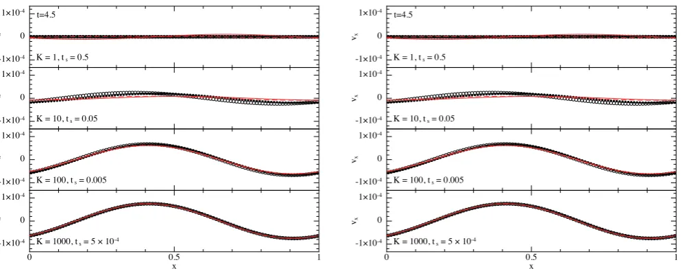
Figure 1. Gas and dust velocities (filled and open circles, respectively) in the dustywave problem using 100 SPH particles and our two implementations of the dust diffusion approximation: two first derivatives (left) and direct second derivatives (right). These may be compared to the analytic linear solution fromLP11 given by the red solid (gas) and dashed (dust) lines. TheL2error is within 6 per cent of the analytic solution forK=100 and within 2 per cent forK=1000, where the diffusion approximation is applicable (here forK42 corresponding tots> tCour=0.012). The solution becomes inaccurate at weaker drag (ts
>0.012). There is no discernible difference between the two implementations, except that the implementation with direct second derivatives (right) is faster.
& Revenga2003; Lodato & Price2010), with only Watkins et al. (1996) suggesting that the two first derivatives approach is more accurate. By comparing our two implementations in Section 4, we effectively compare both approaches. We find only small differ-ences between the two approaches in terms of the overall accuracy, with the main advantages being that the direct second derivatives approach is both faster and easier to implement.
4 N U M E R I C A L T E S T S
A key issue in developing numerical codes for dust–gas mixtures is that there are few simple test problems that can be used to benchmark the algorithm. We have partially resolved this issue by deriving the analytic solution for linear waves in such a mixture (Laibe & Price
2011, hereafterLP11) and showing that the solution for a shock in the limit wherev→0 is the same as for the hydrodynamic case but with a modified sound speed (Miura & Glass1982;LP12a). The dustybox solution (LP11) is not relevant to this paper since we have already assumed thatvhas reached its asymptotic value by using the terminal velocity approximation. Hence, we use the dustywave and dustyshock problems to benchmark our algorithm. Our exploration of the diffusion approximation for dust suggested a new test problem with a simple analytic solution, which we describe in Section 4.3.
4.1 Dustywave
In dustywave problem, we solve for the propagation of a linear wave in a dust–gas mixture. We set up the problem in 1D as in our previous papers (LP12a,b, LP14b), using ρd, 0 = ρg, 0 = 1 (i.e.ρ0= 2 and0= 0.5) with a sinusoidal perturbation to the velocity and density of the mixture particles v(x)=v0sin(2πx) and ρ(x)=ρ0[1+δρ0sin(2πx)], with amplitude v0= δρ0 =1 ×10⁻⁴, with a corresponding thermal energy perturbation given by δu=P0/ρg2,0δρg. An adiabatic equation of state is used with
γ=5/3 and the thermal energy is set so that the initial sound speed
cs=1. We use 100 SPH particles in the domainx∈[0, 1]. There is a fundamental inconsistency in the dustywave initial conditions when using the terminal velocity approximation because the setup of the problem and hence the analytic solution assumes thatv0=0. By definition in the terminal velocity approximation, we havev≡tsf which is non-zero. Hence, the solution even att=0 is not identical to the full one-fluid case. However, these differences become smaller at large drag and at later times.
The numerical solution is shown after 4.5 wave periods in Fig. 1, showing the gas and dust velocities (filled and open cir-cles, respectively). As inLP14b, we have reconstructed the gas and dust velocities on each particle from the barycentric variables, i.e.
vg≡v−vandvd≡v+(1−)v. The left figure shows the results using the two first derivatives approach (Section 3.1) while the right figure shows the results using the direct second derivatives version (Section 3.4) in each case compared to the linear analytic solution fromLP11. There is no distinguishable difference between the two approaches. The solution in the regime where the terminal velocity approximation is valid (K42; lower two panels in each figure, corresponding tots> tCour=0.01) is within a few per cent of the analytic solution. There is a conspicuous phase error at lower drag (K=10 andK=1; first and second rows), in part caused by the inconsistency in the initial conditions, which becomes worse as
tsbecomes larger, and in part because this is where the terminal velocity approximation breaks down. Nevertheless, the general be-haviour in terms of the damping of the wave at intermediate drag is captured despite the inapplicability of the approximation in this regime. The behaviour at even lower drag (K<1; not shown) is incorrect; here the wave remains damped when using the terminal velocity approximation whereas the damping should decrease as the coupling tends to zero. Hence, the full one-fluid approxima-tion should be used in this regime (e.g.LP14b), as we argued in Section 2.2.
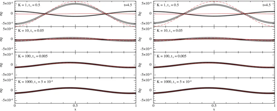
Fig. 2shows the solution for the density perturbation. Impor-tantly, the analytic solution for density in the dustywave problem quickly becomes non-linear, particularly when the drag is weak.
at University of St Andrews on August 13, 2015
http://mnras.oxfordjournals.org/
Figure 2. As in Fig.1but showing the density perturbation. The solution in this case may be compared to the red solid (gas) and dashed (dust) lines, showing a high-resolution non-linear solution computed using the general one-fluid algorithm fromLP14b. The solution is captured with increasing accuracy as the drag becomes stronger, with anL2error of 6 per cent forK=100 and 0.6 per cent forK=1000, but as expected becomes inaccurate in the regime where the approximation breaks down (ts0.012).
This can be seen by considering the limit of no drag. Assuming that the dust is not submitted to any external force, we have
v(t)=v(t=0)=v0sin (kx0), (46)
implying
x(t)=x0−v0sin (kx0)t. (47)
Hence, from mass conservation, the dust density is given by
ρd(t)=
ρd0(x0)
∂∂xx0t =
ρd0(x0) |1−v0kcos (kx0)t|
. (48)
This result is physically consistent with the initial velocity profile: grains are depleted atx= ±π, pile up at x= 0 and maintain a constant density atx= ±π/2 (zero net flux of particles). In par-ticular, density fluctuations become of the order of the background on a typical time (v0k)−1 and the analytic solution of the dusty-wave problem fromLP11 cannot be applied anymore. It should be noted however that the velocities remain small and still agree with the solution of the linear problem. Hence, we have computed the reference solution in Fig.2using a high-resolution (5000 parti-cle) simulation with our fully general one-fluid algorithm (LP14b), whereas in Fig.1 we used the linear solution fromLP11 (both methods produce indistinguishable results for the velocity field).
Since there is no inconsistency in the density in the initial con-ditions, the solution using the diffusion approximation is more ac-curate for the densities than for the velocities (L2error of 0.06 at
K=100 and 0.006 atK= 1000), though it still becomes inac-curate (L2error 0.5) forK≤10. As with the velocities, there is no difference between the two implementations (compare left-and right-hleft-and panels in Fig.2), indicating that any inaccuracies are due to the physical approximation rather than the numerical scheme itself.
4.2 Dustyshock
The dustyshock problem at strong drag was one of the most difficult problems to solve using a two-fluid approach due to the resolution
requirementhcststhat leads to overdamping of the solution if not satisfied (LP12a). We have already shown inLP14bthat this spatial resolution requirement is unnecessary when using a general one-fluid formulation, although the drag still imposes a prohibitive timestep constraint, meaning that an implicit timestepping scheme (albeit a fairly simple one) is still necessary. Fig. 3shows that with our present method we can capture the high-drag dustyshock solution using explicit timestepping without any timestep constraint other than the usual Courant condition, and without any particular spatial resolution requirements.
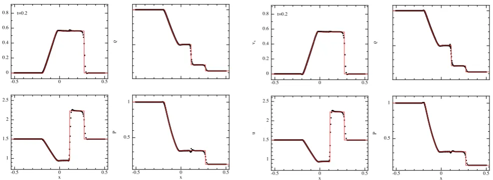
We set up the problem as usual, following the standard Sod (1978) shock tube with conditions in the gas forx≤0 given by (ρg, vg,P)= (1.0, 0.0, 1.0) and forx> 0 given by (ρg,vg,P) =(0.125, 0.0, 0.125). We assume a constant dust fraction in the initial conditions (0=1), using 569 particles (corresponding to a particle spacing ofx=0.001 forx≤0, an adiabatic equation of state withγ=5/3 and a drag coefficientK=1000). In this regime, the solution corresponds to the usual hydrodynamic solution with a modified sound speed (red lines in Fig.3). In this respect, we are testing only the ability of the algorithm to recover the zeroth-order effect of a heavy fluid (seeLP14a), which from the results in Fig.3
can be seen to be true.
As previously there is very little difference between the two im-plementations (comparing left- and right-hand panels) except that the direct second derivatives approach (cf. Section 3.4) produces slightly less noise in the pressure profile across the contact dis-continuity. While this can be important for some problems (see e.g. Price2008), such a minor difference is not enough to prefer this dis-cretization over the two first derivatives approach. However, given that the direct second derivatives algorithm is also significantly faster, it may be preferred on this basis.
4.3 Dustydiffusion
Based on equation (15), we present a new test for dust–gas mixtures with a simple analytic solution. This consists of the steady diffusion of an overconcentration of dust. To set up the problem, we consider a uniform density box withρ=ρ0=1 and an isothermal equation
at University of St Andrews on August 13, 2015
http://mnras.oxfordjournals.org/
Figure 3. Results of the dustyshock test with a large drag coefficient,K=1000, comparing the use of two first derivatives to compute the dust diffusion (left) with the direct second derivative discretization of the diffusion term (right). In both cases, the numerical solutions agree with the analytic solution valid in the limit of infinite drag (solid red line), although the pressure is smoother across the contact discontinuity when the diffusion term is computed directly. The advantage of the present scheme compared to the full one-fluid approach (LP14b) is that we have used explicit timestepping. We also avoid the punitiveh< tscsresolution requirement associated with the two-fluid formulation (LP12a). 569 SPH particles were used.
of stateP =c2
sρgwithcs=1. In this case, the dust diffusion can be described by equation (15). For the diffusion parameter, we assume that the stopping time is a constant (this is equivalent to assuming an Epstein-like drag, wherets=ρgrainsgrain/(ρcs) is constant).
4.3.1 Analytic solution
The exact solution can be obtained by solving the equation
d
dt = ∇ ·(η˜∇), (49)
where ˜η≡tscs2is a constant. We solve this by assuming spherical symmetry, i.e.
d dt =
˜
η r2
d dr
r2d dr
, (50)
for which there are several known analytic solutions, including the general time-dependent solution
(r, t)=A|10 ˜ηt+B|−35− r 2
10 ˜ηt+B, (51)
whereAandBare arbitrary constants. We use this solution to verify our numerical scheme by solving only the diffusion equation via either equations (26) and (30) or equation (43), with the particle positions fixed (for this problem only).4
4.3.2 Results
We set up the problem in 3D with 50×58×60 particles set on a uniform close-packed lattice in the domainx,y,z∈[−0.5, 0.5]. The positions of theyandzboundaries are adjusted slightly to ensure
4We attempted to construct an equilibrium situation involving all of equa-tions (10)–(12), for example a hydrostatic equilibrium in a fixed potential. However, it is difficult to construct an equilibrium where the dust simply diffuses according to equation (49) because the change tocauses a change to the pressure gradient and hence causes an acceleration to the barycentre also.
periodicity of the lattice across the boundary (the particle spacing inx,yandzisp,√3p/2 and√6p/3, respectively, wherep
=0.02). We use an isothermal equation of state, settingcs=1 and
ts=0.1 such that ˜η=0.1, and set the initial dust fraction using
(r,0)=0
1−
r rc
2
, (52)
consistent with equation (51) withB≡0/rc2andA≡0B 3 5. We set0=0.1 andrc=0.25.
Fig.4compares the numerical solution to the analytic solution, while Fig.5illustrates the general behaviour of the solution. The solution with equation (43) (right-hand panel of Fig.4) is excellent (L2error5×10−4forr<0.2), apart from the physical deviation from the self-similar solution due to the transition to constant rather than negativeat the outer radius. The solution with using equations (26) and (30) (left-hand panel) is also good, but shows some low-amplitude oscillations that develop from the propagation of the ‘kink’ in the initial epsilon profile. These oscillations are worse at lower resolution [they can be smoothed out by adding some artificial dissipation inbut the solution is still not as good as using equation (43)].
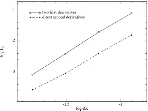
Fig.6quantifies these results with a convergence study using 83, 163, 323or 643particles arranged on a cubic lattice. We show theL
2 error computed bySPLASH(Price2007) from particles withr<0.2. While in both cases the convergence is of second order∝(x)2, it can be seen that the direct second derivatives approach gives results more accurate by a factor of 5 at any given resolution. Our results with both schemes when employingsinstead of(Appendix B) are worse by a factor of∼2, again with a similar preference for the direct second derivatives approach. Thus, while it is clear that all of our proposed numerical schemes correctly discretize the diffusion equation, we find the discretization using equation (43) to be more accurate for this problem.
4.4 Dust settling in a protoplanetary disc
Our final test is drawn from our intended application, namely the dynamics of small grains in protoplanetary discs.
at University of St Andrews on August 13, 2015
http://mnras.oxfordjournals.org/
Figure 4. Dust fraction as a function of spherical radius in the 3D dust diffusion test att=0.0, 0.1, 0.3, 1, 3 and 10 (top to bottom) from simulations using 50 ×58×60 particles. The numerical solution, projecting all particles inr, is given by the black dots and may be compared to the analytic solution given by the red lines. The left-hand panel shows the solution with two first derivatives, while the right-hand panel uses the direct second derivative.
Figure 5. Cross-section of the dust density in thez=0 plane in the 3D dust diffusion test att=0, 1 and 10 (left to right).
4.4.1 Setup
We simplify the problem by considering only the vertical settling of grains in ther–zplane. That is, we set up particles in a two-dimensional Cartesian box with an acceleration in the ‘vertical’ (z) direction given by
az= −z GM
R2 0+z2
3 2
, (53)
where we assume code units such thatGM=1 and setR0= 5 as a constant. The boundary conditions are periodic in the hori-zontal (x) direction and free in the vertical direction. We use an isothermal equation of stateP =c2
sρ, where the sound speedcs is set such that the aspect ratioH /R0≡c2s/( 0R0)=0.05, where
0≡
GM/R3
0. The orbital time is thereforetorb≡2π/ 0≈70 in code units. We set particles of equal mass initially on a uni-form hexagonal lattice in the domain x ∈ [−0.25, 0.25] and
z∈[−3H, 3H]. We specify the particle separation in thexdirection to be either 16, 32 or 64, resulting in 16×56=856 particles at the lowest resolution, 32×111=3552 particles at medium resolution and 64×222=14 208 at the highest resolution.
We then stretch the particle distribution to match the equilibrium density profile using the method described in Price (2004) where thezposition of each particle is determined by solving the root finding problem
f(z)= M(z)
M(zmax)
− (z0−zmin)
zmax−zmin
=0, (54)
Figure 6. Convergence in the dust diffusion problem, showingL2 error for the solution withinr<0.2 as a function of the particle spacing. While both methods show second-order convergence, the direct second derivatives solution is more accurate because of oscillations in the two first derivatives approach propagating from the ‘kink’ in the initialprofile seen in Fig.4.
whereM(z)≡zz minρ(z
)dz,z
0is the initial position of the particle and we set
ρ(z)=ρ0exp[−z2/(2H2)]. (55)
We set the mass of each particle equal toM(zmax) divided by the number of particles in the domain, consistent with the desired den-sity profile. Equation (55) is a slight approximation (fourth order inz/H; e.g. Laibe, Gonzalez & Maddison2012) but this is unim-portant since we relax the particles into a hydrostatic equilibrium anyway, as described below.
We set up the simulation initially with only gas and run the calculation tot=1000 in code units (i.e.∼14 orbits) with both artificial viscosity and an artificial damping term of the form
dv dt
damp
= −fdampv, (56)
at University of St Andrews on August 13, 2015
http://mnras.oxfordjournals.org/
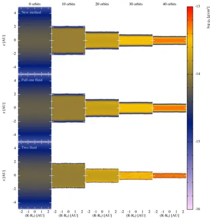
[image:9.595.46.284.284.360.2]Figure 7. Settling of mm dust grains in a 2D (r–z) vertical section of a protoplanetary disc atR0=50 au (assumingH/R=0.05; soH0=2.5 au) using 32× 111 mixture particles. The plot shows dust density as a function of time. The top row shows the results using our new dust diffusion method. The solution may be compared to that obtained with the full one-fluid formulation from LP14b (middle row) and with the two-fluid formulation fromLP12aandLP12b(bottom row; uses 32×111 particles in both gas and dust). Our new method requires half the number of particles compared to the two-fluid approach and is 50 times faster.
wherefdamp = 0.03 in order to allow the distribution to relax to equilibrium. We then add dust to the simulation, assuming a dust-to-gas ratio ofρd/ρg=0.01 by setting the dust fraction using
≡ ρd
ρ =
ρd/ρg (1+ρd/ρg)
. (57)
We then evolve the simulation for a further 50–100 orbits. To give the problem physical meaning, we consider a distance unit of 10 AU (such thatR0=5 corresponds to 50 au), a mass unit of 1 Mand the time unit set such thatG=1 in code units. This implies an orbital time of 2π/ 0=353 yr. A mid-plane density
ρ0of 10−3in code units then corresponds to≈6×10⁻¹³g cm−3, giving a disc surface density ≈55 g cm−2. We adopt a linear Epstein drag prescription, defining the stopping time according to
equation (20). We set the intrinsic grain densityρgrain=3 g cm−3. The mid-plane stopping time atR0is given by
ts 0=1.35×10⁻³
s
grain 1 mm
ρgrain 3 g cm−3
ρ ρ0
−1
. (58)
4.4.2 Settling of millimetre grains
We first perform a series of tests with a grain size ofsgrain=1 mm, chosen as a balance between the regime where the diffusion method is applicable and where it is still possible to obtain a solution in a reasonable time with the two-fluid method. For the setup above, this is at the limit of where the diffusion method is applicable,
at University of St Andrews on August 13, 2015
http://mnras.oxfordjournals.org/
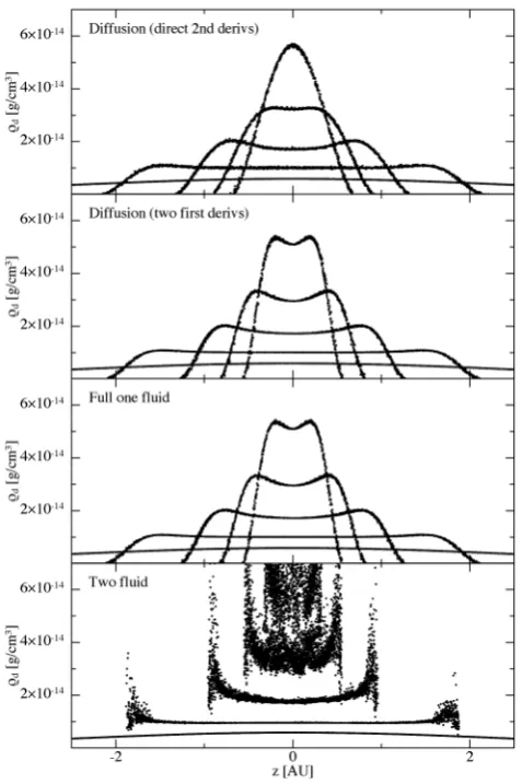
Figure 8. As in Fig.7but showing the projection of dust density on all particles in 2D as a function ofz, plotted att=0, 10, 20, 30 and 40 orbits for the different methods. The direct second derivatives formulation (top) gives a slightly more smoothed result compared to the two first derivatives method (second row), the latter of which is indistinguishable from the solution with the full one-fluid method (third row). The one-fluid methods are less well resolved in the dust density for this problem but give a significantly less noisy solution than obtained with the two-fluid method (bottom). The diffusion method is 50 times faster at this resolution and grain size, with increasing performance gains for smaller grains.
and indeed we found that equation (16) controlled the timestep, indicating that the time dependence of the differential velocity has started to become important. In LP12a, we showed that it was necessary to satisfyhcststo avoid overestimating the drag. For 1 mm grains, our two-fluid calculations violate this criterion by a factor of∼9, 4.5 and 2.25 at the mid-plane at low, medium and high resolution, respectively, but do not appear to show overdamping. Lor´en-Aguilar & Bate (2014) found that the resolution problem is not as severe when the dust-to-gas ratio is low, suggesting thath≤
cstsis a more precise resolution criterion.
[image:11.595.310.550.58.234.2]Fig.7shows the dust density in the medium-resolution calcula-tions at intervals of 10 orbital periods using three different methods. The top row shows the results with our new method employing the two first derivatives approach (Section 3.1). The results with direct second derivatives (equation 43) are similar but slightly less well resolved (see Fig.8). The second row of Fig.7shows the solution obtained with the general one-fluid method fromLP14b. The main difference is that the differential velocityvis explicitly evolved in that formulation, and so there is a timestep constraint from the
Figure 9. Resolution study in 1D version of dust settling problem (Figs7 and8), showing solution after 30 orbits using the diffusion approximation with direct second derivatives (top left), two first derivatives (top right), the one-fluid method fromLP14b(bottom left) and the two-fluid method (bottom right). The particle number refers to the total number of particles in the domain in each case. In the one-fluid methods, the resolution follows thetotalmass rather than the dust mass, so the dust density is comparatively less well resolved.
stopping time which makes the simulation run∼25 times slower for this grain size when computed with only explicit timestepping with the constraintt<ts. With the diffusion approximation, the timestep constraint isinverselyproportional to the stopping time al-though quadratically proportional to resolution (equation 16). The third row shows the solution obtained with the two-fluid algorithm (LP12a). In this case, instead of setting the dust fraction, we added a separate set of dust particles copied from the gas particles but with 1 per cent of the mass. This approach therefore required twice the number of particles compared to our diffusion algorithm and the timestep is also constrained by the stopping time. Computing this solution required approximately 50 times more CPU time than the diffusion method.
All four methods produce dust settling on a comparable time-scale, with only minor differences in the numerical solutions. A more detailed comparison is given in Fig.8, showing the dust den-sity on all particles as a function ofzat the same times as those shown in Fig. 7. The main noticeable difference is that the two-fluid solution contains more noise in the particle distribution. This is because the dust is modelled as a separate set of particles that feel no mutual repulsion, compared to the one-fluid case where the dust distribution benefits from the regular arrangement of the mix-ture particles. The approach with direct second derivatives (top row) produces a slightly oversmoothed solution compared to the two first derivatives approach (second row) – with the latter giving results that are indistinguishable from the full one-fluid method (third row), showing that the diffusion approximation is indeed accurate in this regime.
A major difference between the one-fluid method and the two-fluid method is that resolution is tied to thetotalmass rather than the dust mass. This is evident in Fig.8where the two-fluid method (bottom row) can be seen to better capture the ‘wings’ in the dust density at high latitudes. We quantify this further in Fig.9with a resolution study of the same problem performed in 1D to avoid the particle noise in the two-fluid approach. Settling means that after some time the dust covers a much smaller region of the domain than the gas, so the one-fluid formulations under-resolve the dust
at University of St Andrews on August 13, 2015
http://mnras.oxfordjournals.org/
Figure 10. As in Fig.7but comparing settling of grains of different sizes in a vertical section of a protoplanetary disc at 50 au. Each panel shows the dust density after 50 orbits computed with our new method (similar results are found with both implementations described in this paper). The decrease in settling time with increasing grain size (left to right) is clearly evident. Simulations in this regime are prohibitively slow with the two-fluid approach. We used explicit timestepping in all cases, with the simulations for grain sizes of<1 mm constrained only by the Courant condition.
compared to the two-fluid method, since resolution is tied to the total mass, most of which remains at high latitudes. By contrast, in the two-fluid approach resolution is tied to the dust mass and so is naturally placed towards regions of high dust density. This is both an advantage and a disadvantage to both types of approaches; it depends on whether it is desirable to resolve the total mass or the dust mass. This point is discussed inLP14bmainly as an advantage to the one-fluid method since it avoids the possibility of dust particles becoming ‘trapped’ below the resolution of the gas.
In obtaining our results with the diffusion approximation, we found a few caveats to the numerical algorithm we derived in Sec-tion 3. First, we found it necessary with both to use theM6kernel for this problem to obtain a smooth and accurate solution (this kernel extends to 3hinstead of 2hand so better approximates the Gaus-sian). To avoid particle pairing occurring at high latitudes with the quintic, we set the ratio of smoothing length to particle spacing to 1.0 instead of 1.2, equivalent to using a mean neighbour number of 28.3 in 2D (see Price 2012). The second caveat was that the dust fraction becomes negative around the edge of the collapsing dust layer in both of our implementations (and also with the full one-fluid method). This arises because of the exact conservation of the dust mass in the algorithm, which causes a slight overshoot at the discontinuity. In order to smoothly handle this, we derived an alternative approach (Appendix B) which guarantees a positive dust fraction, but we found it to give less accurate results than the method employing(cf. Section 4.3). Instead, we found that the most effective way of solving this was to simply set the dust frac-tion to zero on particles where it had become negative. This slightly violates the exact conservation of the dust mass, but the error is small (∼10−5inwith the quintic) and it is a small price to pay for stability of the algorithm.
4.4.3 Settling with different grain sizes
Finally, we demonstrate the ability of the diffusion method to sim-ulate small grains in a protoplanetary disc by performing a series of calculations varying the grain size from 0.1μm to 1 mm. Grain
sizes below 1 mm are difficult to simulate at all with the two-fluid technique because of the punitive spatial and temporal resolution requirements (LP12a,b). With the general one-fluid method pre-sented inLP14b, the limitation on the spatial resolution is removed, because we are no longer modelling the separation between fluids with physically separate resolution elements, but it is still neces-sary to use implicit timestepping. Yet these grains are important in protoplanetary discs as they control much of the thermal radiation. Fig.10shows the results of a series of medium-resolution (32 ×111) calculations of dust settling for different grain sizes, shown after 50 orbits atR0. We used only explicit timestepping, and for grain sizes smaller than 1 mm the timestep was constrained only by the Courant condition. The different settling behaviour of the dif-ferent grain populations in discs is clearly evident, with the micron and submicron grains remaining stuck to the gas at high latitudes, the millimetre grains settling effectively to the mid-plane and the 100 and 10μm grains having partially settled.
To accurately and efficiently simulate single-size small grains in discs in this manner is the first step towards modelling an evolving grain population self-consistently.
5 D I S C U S S I O N A N D C O N C L U S I O N S
We have derived and implemented a numerical scheme for describ-ing the dynamics of small dust grains coupled to a gas, usdescrib-ing SPH, in the limit where the stopping time is short compared to the com-putational timestep. This requires solving one additional diffusion equation as well as the usual equations of hydrodynamics slightly modified by some additional terms. We derived two implementa-tions, one where the diffusion equation is computed using two first derivatives (Section 3.1) and one where direct second derivatives were employed (Section 3.4). We found only minor differences be-tween the two approaches on the test problems we tried. Given this, we recommend the direct second derivatives approach (Section 3.4), which is both simpler and faster because it does not require an extra loop over the particles.
at University of St Andrews on August 13, 2015
http://mnras.oxfordjournals.org/
As discussed in Section 2.2, the terminal velocity approxima-tion or, as we prefer, the ‘diffusion approximaapproxima-tion for dust’ is valid when the stopping time is less than the computational timestep. The simple way to guarantee this validity in practice is to ensure that the diffusion timestep (equation 16) is not constraining the timestep, otherwise the more general one-fluid approach imple-mented inLP14bwhere the time dependence ofvis kept should be used instead. In this sense, the method we have described is complementary to both the full one-fluid approach (LP14b) and the two-fluid approach (LP12a). The main difference is that the other methods need implicit timesteps when the grain size issmall(ts<
t), whereas this method requires implicit timesteps when the grain size islarge(ts> t), but this is where the approximation breaks down anyway.
Finally, we considered only one grain size at a time in this paper. We have recently generalized our one-fluid formulation to describe an arbitrary number of grain populations all within a single fluid mixture (Laibe & Price2014c). Our next step will be a numeri-cal implementation of this more general formulation, including the simplification to a diffusion approximation, as well as modelling the evolution of the grain population including growth and frag-mentation.
AC K N OW L E D G E M E N T S
DJP is very grateful for funding via an Australian Research Council (ARC) Future Fellowship, FT130100034, and Discovery Project grants DP1094585 and DP130102078. GL acknowledges funding from the European Research Council via FP7 ERC advanced grant project ECOGAL. We thank Mark Hutchison, Joe Monaghan and Giovanni Dipierro for useful discussions, and the anonymous ref-eree for comments that improved the paper. We usedSPLASHfor the figures and renderings (Price2007).
R E F E R E N C E S
Ayliffe B. A., Laibe G., Price D. J., Bate M. R., 2012, MNRAS, 423, 1450 Barranco J. A., 2009, ApJ, 691, 907
Brookshaw L., 1985, PASA, 6, 207 Chiang E., 2008, ApJ, 675, 1549
Cleary P. W., Monaghan J. J., 1999, J. Comput. Phys., 148, 227 Cullen L., Dehnen W., 2010, MNRAS, 408, 669
Espa˜nol P., Revenga M., 2003, Phys. Rev. E, 67, 026705
Flebbe O., Muenzel S., Herold H., Riffert H., Ruder H., 1994, ApJ, 431, 754 Jacquet E., Balbus S., Latter H., 2011, MNRAS, 415, 3591
Laibe G., Price D. J., 2011, MNRAS, 418, 1491 (LP11) Laibe G., Price D. J., 2012a, MNRAS, 420, 2345 (LP12a) Laibe G., Price D. J., 2012b, MNRAS, 420, 2365 (LP12b) Laibe G., Price D. J., 2014a, MNRAS, 440, 2136 (LP14a) Laibe G., Price D. J., 2014b, MNRAS, 440, 2147 (LP14b) Laibe G., Price D. J., 2014c, MNRAS, 444, 1940
Laibe G., Gonzalez J.-F., Maddison S. T., 2012, A&A, 537, A61 Lee A. T., Chiang E., Asay-Davis X., Barranco J., 2010, ApJ, 718, 1367 Lodato G., Price D. J., 2010, MNRAS, 405, 1212
Lor´en-Aguilar P., Bate M. R., 2014, MNRAS, 443, 927 Miura H., Glass I. I., 1982, Proc. R. Soc. Lond. A, 382, 373 Monaghan J. J., 2005, Rep. Prog. Phys., 68, 1703
Morris J. P., Monaghan J. J., 1997, J. Comput. Phys., 136, 41 Pandey B. P., Wardle M., 2008, MNRAS, 385, 2269
Price D. J., 2004, PhD thesis, Univ. Cambridge, Cambridge, UK Price D. J., 2007, PASA, 24, 159
Price D. J., 2008, J. Comput. Phys., 227, 10040 Price D. J., 2012, J. Comput. Phys., 231, 759 Price D. J., Federrath C., 2010, MNRAS, 406, 1659
Price D. J., Monaghan J. J., 2004, MNRAS, 348, 139 Price D. J., Monaghan J. J., 2007, MNRAS, 374, 1347 Sod G. A., 1978, J. Comput. Phys., 27, 1
Wadsley J. W., Veeravalli G., Couchman H. M. P., 2008, MNRAS, 387, 427 Watkins S. J., Bhattal A. S., Francis N., Turner J. A., Whitworth A. P., 1996,
A&AS, 119, 177
Youdin A. N., Goodman J., 2005, ApJ, 620, 459
A P P E N D I X A : P R O O F T H AT E Q UAT I O N ( 4 5 ) I S A D I S C R E T E F O R M O F E Q UAT I O N ( 1 3 )
Here, we prove that the expression obtained for the second term in equation (45) by enforcing the conservation of energy, namely
1 2(1−a)ρa
b
mb
ρb
(ua−ub)(Da+Db)(Pa−Pb)Fab
|rab|,
(A1)
is indeed a discrete form of the corresponding term in equation (13), i.e.
−ts
ρg
∇P · ∇u. (A2)
We proceed, following Price (2012), by identifying−2Fab/|rab|as
equivalent to the second derivative of a (new) kernel function, i.e.
∇2Y
ab≡ −2Fab
|rab| . (A3)
It may be shown straightforwardly that this new kernelYabindeed
satisfies the normalization conditions appropriate to the kernel sec-ond derivative (see Price2012for more details). We can then take the Laplacian of the standard SPH summation interpolant with this kernel, i.e.
Aa
b
mbAρb
bYab, (A4)
to give
∇2A
a
b
mbAρb b∇
2Y
ab. (A5)
By writing equation (A1) in the form
− 1 4ρga
b
mb
ρb(ua−ub)(Da+Db)(Pa−Pb)∇
2Y
ab, (A6)
we can then use equation (A5) to translate the various terms. Ex-panding equation (A6), we have
− 1 4ρga
b
mb
ρb (PauaDa−PaubDa+PauaDb−PaubDb
−PbuaDa+PbubDa−PbuaDb+PbubDb)∇2Yab. (A7)
Translating each of the terms in turn using equation (A5) gives
− 1 4ρg
P uD∇2
1−P D∇2u+P u∇2D−P∇2(uD)−uD∇2P
+D∇2
(P u)−u∇2(P D)+ ∇2(P uD). (A8)
Expanding the∇2(ab) terms using the vector identity
∇2(ab)=a∇2b+2(∇a· ∇b)+b∇2a, (A9)
and expanding the last term using
∇2(P uD)=uD∇2P+P D∇2u+P u∇2D+2u(∇P· ∇D) +2D(∇P · ∇u)+2P(∇D· ∇u), (A10)
at University of St Andrews on August 13, 2015
http://mnras.oxfordjournals.org/