Machine learning for systems pathology

Wim Verleyen

A Thesis Submitted for the Degree of PhD

at the

University of St Andrews

2013

Full metadata for this item is available in

Research@StAndrews:FullText

at:

http://research-repository.st-andrews.ac.uk/

Please use this identifier to cite or link to this item:

http://hdl.handle.net/10023/4512

PhD Thesis

Machine Learning for Systems Pathology

by

Wim Verleyen

Abstract

Systems pathology attempts to introduce more holistic ap-proaches towards pathology and attempts to integrate clinicopatho-logical information with “-omics” technology. This doctorate re-searches two examples of a systems approach for pathology: (1)a personalized patient output prediction for ovarian cancerand (2)an an-alytical approach differentiates between individual and collective tumour invasion.

During the personalized patient output prediction for ovarian cancer study, clinicopathological measurements and proteomic biomarkers are analysed with a set of newly engineered bioinfor-matic tools. These tools are based upon feature selection, survival analysis with Cox proportional hazards regression, and a novel Monte Carlo approach. Clinical and pathological data proves to have highly significant information content, as expected; however, molecular data has little information content alone, and is only sig-nificant when selected most-informative variables are placed in the context of the patient’s clinical and pathological measures. Fur-thermore, classifiers based on support vector machines (SVMs) that predict one-year PFS and three-year OS with high accuracy, show how the addition of carefully selected molecular measures to clini-cal and pathologiclini-cal knowledge can enable personalized prognosis predictions. Finally, the high-performance of these classifiers are validated on an additional data set.

A second study, an analytical approach differentiates between individual and collective tumour invasion, analyses a set of morpho-logical measures. These morphomorpho-logical measurements are collected with a newly developed process using automated imaging analysis for data collection in combination with a Bayesian network analysis to probabilistically connect morphological variables with tumour in-vasion modes. Between an individual and collective inin-vasion mode, cell-cell contact is the most discriminating morphological feature. Smaller invading groups were typified by smoother cellular sur-faces than those invading collectively in larger groups. Interestingly, elongation was evident in all invading cell groups and was not a specific feature of single cell invasion as a surrogate of epithelial-mesenchymal transition. In conclusion, the combination of auto-mated imaging analysis and Bayesian network analysis provides an insight into morphological variables associated with transition of cancer cells between invasion modes. We show that only two morphologically distinct modes of invasion exist.

Declarations

I, Wim Verleyen, hereby certify that this thesis, which is approxi-mately 72,500 words in length, has been written by me, that it is the record of work carried out by me and that it has not been submitted in any previous application for a higher degree. I was admitted as a research student in August 2008 and as a candidate for the degree of PhD in August 2009; the higher study for which this is a record was carried out in the University of St Andrews between 2009 and 2012.

date__________________ signature of candidate

I hereby certify that the candidate has fulfilled the conditions of the Resolution and Regulations appropriate for the degree of PhD in the University of St Andrews and that the candidate is qualified to submit this thesis in application for that degree.

date__________________signature of supervisor

In submitting this thesis to the University of St Andrews we un-derstand that we are giving permission for it to be made available for use in accordance with the regulations of the University Library for the time being in force, subject to any copyright vested in the work not being af fected thereby. We also understand that the title and the abstract will be published, and that a copy of the work may be made and supplied to any bona fide library or research worker, that my thesis will be electronically accessible for personal or re-search use unless exempt by award of an embargo as requested below, and that the library has the right to migrate my thesis into new electronic forms as required to ensure continued access to the thesis. We have obtained any third-party copyright permissions that may be required in order to allow such access and migration, or have requested the appropriate embargo below.

The following is an agreed request by candidate and supervisor regarding the electronic publication of this thesis: Embargo on both Chapter 3 and 5 of printed copy and electronic copy for the same fixed period of 2 years on the following ground(s): publication would preclude future publication.

date__________________ signature of candidate

Acknowledgements

During the course of my PhD studies, there were many people that had a great contribution to the outcome of my work.

First, I would like to thank my main supervisor V. Anne Smith. She has been a great mentor during my time in St Andrews. I am very grateful for many opportunities to follow my scientific inter-ests. I really enjoyed the confidence and support in situations I was not so sure about the outcomes of my work. I really need to thank her for her persistent patience and inspiring advice that have de-fined a standard for me which I will try to emulate when I supervise students.

To my thesis committee, thank you for being engaged during the process of my doctorate. I have been fortunate to receive guidance, and plenty of suggestions which have inspired me to improve my research into many directions.

I need to thank the Division of Pathology at the University of Edinburgh for their contribution. Prof. David Harrison, Dr. Dana Faratian, and many more have been treating me as being a part of their research group whenever I needed their advice, infrastructure, and data.

I would like to thank SIMBIOS at the University of Abertay Dundee. Prof. James Bown, Dr. Mark Showman, Mr. Michael Id-owu, and many more to be always very knowledgeable and infor-mative in the course of this study.

I would like to convey thanks to the Scottish Universities Life Sciences Alliance (SULSA), the School of Biology of the University of St Andrews, and Prof. David Harrison for funding my doctorate studies.

Finally, I want to thank my family and friends for their love and support. And most of all for my supportive, encouraging, and in-spiring girlfriend Olivia for her patient and understanding during the final stages of the Ph.D. is so appreciated.

1

Introduction

13

1.1

Machine learning

14

1.1.1

Probabilistic graphical models

15

1.1.2

Survival analysis

15

1.2

Systems pathology

17

1.2.1

Clinicopathological definition of a tumour

18

1.2.1.1

Tumour grading

18

1.2.1.2

Tumour staging

19

1.3

Cancer

20

1.3.1

Breast cancer

25

1.3.2

Ovarian cancer

27

1.4

Application of systems approach in pathology

28

1.5

Layout of the thesis

30

2

Choice of methodology

31

2.1

Computational methodologies

32

2.1.1

Bayesian networks

33

2.1.1.1

Conditioning

35

2.1.1.2

Marginalization

35

2.1.1.3

Factor

35

2.1.1.4

Chain rule for Bayesian networks

35

2.1.1.5

Independence

36

2.1.1.6

Conditional independence

36

2.1.1.7

Active trail

36

2.1.1.8

d-separation

37

2.1.1.9

Static Bayesian network

38

2.1.1.11

Dynamic Bayesian network (DBN)

39

2.1.1.12

Structure learning

40

2.1.1.13

Data discretization

44

2.1.1.14

Data requirements

45

2.1.1.15

Heuristic search methods

45

2.1.1.16

Model averaging

46

2.1.1.17

Influence score

46

2.1.2

Linear models

47

2.1.2.1

General Linear Model (GLM)

48

2.1.2.2

Model selection

50

2.1.2.3

Feature selection

51

2.1.2.4

Regularization

52

2.1.2.5

Performance measures for linear models

52

2.1.2.6

Interactions

52

2.1.2.7

Generalized Linear Models (GeLM)

53

2.1.3

Support vector machines (SVM)

54

2.1.3.1

Statistical learning theory

55

2.1.3.2

Lagrangian formulation

58

2.1.3.3

Support vector machines in the linear separable case

60

2.1.3.4

Support vector machines in the linear non-separable case

63

2.1.3.5

Support vector machines in non-linear case

65

2.1.3.6

SVM for regression

67

2.1.3.7

Nonlinear SVM regression

70

2.1.3.8

Other SVM formulations

70

2.1.3.9

Feature selection for SVM regression

70

2.1.4

Survival analysis

71

2.1.4.1

Terminology

71

2.1.4.2

Non-parametric approaches

74

2.1.4.3

Semi-parametric models

75

2.1.4.4

Feature selection

78

2.1.4.5

Concordance index

80

2.1.4.6

Partial Cox regression (PCR)

81

2.1.5

Resampling methods

82

2.1.5.1

Bootstrapping

82

2.1.5.2

Monte Carlo sampling

83

2.1.5.3

Cross validation procedures

83

2.1.5.4

Performance measures for classification

83

2.2

Biological methodologies

86

2.2.1

Reverse phase protein array (RPPA)

86

2.2.2

Protein expression in tissue microarray (TMA)

87

3

Ovarian cancer

89

3.1

Data collection

90

3.1.1

Clinicopathological variables

90

3.1.1.1

Clinicopathological inputs for model building

90

3.1.1.2

Clinicopathological outputs for model building

91

3.1.2

Proteomics profile

93

3.2

Machine learning

94

3.2.1

Bayesian networks

95

3.2.1.1

Bayesian network of the proteomics profile

96

3.2.1.2

Bayesian network of the clinicopathological measurements

96

3.2.1.3

Bayesian network of the clinicopathological measurements and the proteomics profile

97

3.2.2

Survival analysis

102

3.2.2.1

Feature selection

102

3.2.2.2

Feature selection for the clinicopathological data segmentation

109

3.2.3

Classification

114

3.2.3.1

One-year progression-free survival (1YM-PFS)

115

3.2.3.2

Three-year overall survival (3YM-OS)

117

3.3

Validation

119

3.3.1

Quantitative fluorescence image analysis

119

3.3.2

One-year model of progression-free survival

121

3.3.2.1

10-fold cross validation

121

3.3.2.2

Validation based on separate data set

122

3.3.3

Three-year model of overall survival

123

3.3.3.1

10-fold cross validation

123

3.3.3.2

Validation based on separate data set

124

3.4

Discussion

124

4

Morphology during tumour invasion

127

4.1

Tumour invasion

128

4.2

Automated image analysis

129

4.3

Bayesian network

131

4.4

Discriminative capacity of morphological measures

132

4.4.1

Cell-cell contact

133

4.4.2

Group area

133

4.4.3

Surface roughness

134

4.4.4

Length

/

width ratio

135

4.5

Discussion

135

5

Conclusion

137

5.1

Contributions

137

5.1.1

Biomarker discovery for ovarian cancer

137

5.1.2

Tumour invasion

138

5.2

Future work

138

5.2.1

Biomarker discovery for ovarian cancer

138

5.2.2

Tumour invasion

139

6

Bibliography

141

7

Appendix A: data sets

161

7.1

Edinburgh Ovarian Cancer Register (EOCR)

161

7.1.1

Original data set for feature selection and training set for 1YM-PFS and 3YM-OS classifiers

161

7.1.2

Additional validation data set for the validation of 1YM-PFS and 3YM-OS classifiers

161

7.2

Tumour invasion data set

162

1.1 Schematic view of generative machine learning. 14

1.2 Schematic view of discriminative machine learning. 14

1.3 An example of the survival function for the progression-free sur-vival (PFS) for patients under different treatment regimens (Reg-imen 1: platinum and Reg(Reg-imen 2: platinum combined with taxane). The grey area indicates the 95% confidence interval (see also sec-tion 2.1.2.1 on page 49). 16

1.4 Systems biology block scheme. 17

1.5 An overview of of known biological circuits active during cancer. The figure is constructed from [Hanahan and Weinberg, 2000, Hana-han and Weinberg, 2011]. 21

1.6 Mammary ductal network (Modified from: [Med, 2008]). This duc-tal network is analysed to detect the stage of breast cancer. 26

1.7 Hierarchical clustering applied for the gene expression data (From Fig. 1 of Sorlie et al [Sorlie et al., 2001]). 27

1.8 A pyramid for system biology illustrates the bottom-up and top-down approaches. 28

2.1 A simple example of a Bayesian network to illustrate fundamen-tal concepts. 35

2.2 A simple example of a Bayesian network to illustrate the conditional distribution probabilities (CPD) that are part of the chain rule. 35

2.3 The Bayesian network example were thev-structureis indicated. 37

2.4 Statistical dependencies in a Bayesian network a top-down infor-mation flow (causal reasoning). 37

2.5 Statistical dependencies in a Bayesian network a bottom-up infor-mation flow (evidential reasoning). 37

2.6 Statistical dependencies in a Bayesian network with aXi−₁←−X_i−→ Xi+1(inter-causal reasoning). 37

2.7 A trail in a Bayesian network that combines different types of rea-soning. 37

2.8 DBN representation for an underlying causal network with loop. 40

2.9 Geometrical interpretation of Lagrangian multiplier. 58

2.10 Support vector machine (SVM) in the linear separable case. 61

2.11 Support vector machine (SVM) in the non-separable case. 64

2.12 The soft margin loss for SVM regression [Smola and Schölkopf, 2004]. 67

2.14 Analysis of the proportional hazards assumption withcox.zph func-tion in R. The flatness of the fitted line illustrates that the Stage pa-rameter does now violates the proportional hazards assumption over the survival time (Time). 78

2.15 Forward phase protein array and reverse phase protein array have a different configuration of analytes and antibodies. 86

2.16 An example of an RPPA two-by-two grid plate. A set of 9 proteins are measure for a time-series with 17 intervals. Each dot on the fig-ure represents the expression of an antibody of a corresponding tar-get. 87

2.17 Immunofluorescence images of a tissue microarrays assay (Blue= DAPI nuclei; Green=cytokeratin tumour mask Red= antibody-conjugated flourophores) (From Fig. 1 of Faratian et al. [Faratian et al., 2011]). 88

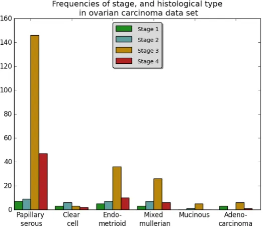
3.1 Frequencies of stages, and histological types in the data. Not all the different combinations of stage and histological type are equally dis-tributed in this data set. Later stage ovarian carcinoma have a higher frequency compared to the early stage ovarian cancer. 91

3.2 The difference in time between overall survival (OS), and progression-free survival (PFS) (Dx,Sx: date of histological diagnosis,CRx: date of treatment diagnosis,Re/Prog: date of first signs of disease recur-rence,DLS/Death: date of death from any cause). 91

3.3 A survival function for the progression-free survival (PFS) and over-all survival (OS) for patients under different treatment regimen (Reg-imen 1: platinum and Reg(Reg-imen 2: platinum combined with taxane). 92

3.4 The biological circuit of known interactions active in the proteomics profile for ovarian cancer [Hanahan and Weinberg, 2000,Hanahan and Weinberg, 2011]. 94

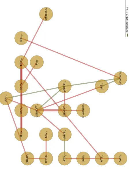
3.5 Bayesian network of the proteomics profile. 98

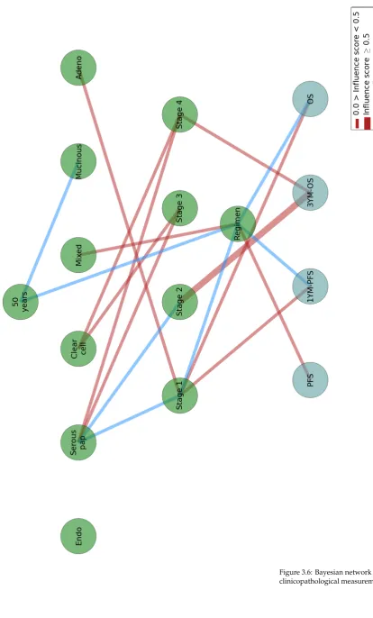
3.6 Bayesian network of the clinicopathological measurements. 99

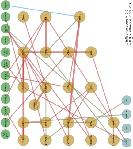
3.7 Three-layered Bayesian network with a first layer of clinicopatho-logical measurements, a second layer of candidate proteomes biomark-ers, and third layer of progression-free survival (PFS) and overall survival (OS) outputs. 100

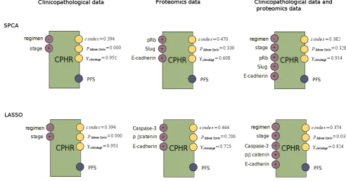
3.8 The following scheme illustrates the different discriminative ma-chine learning methodologies used during this research: survival analysis and classification. First, feature selection is executed on the clinicopathological, proteomics data, and the combination of both. The selected features are plugged into the survival analysis, and into the classification model. The survival model is verified with the fol-lowing performance measure: c-index, p value of a Monte Carlo ex-periment, and the shrinkage. The classification models are verified with area under ROC curve (AUC), a hybrid metric (SAR), and precision-recall F measure (F). 101

3.10 The Monte Carlo distribution and the performance measures: 10-fold cross validated c-index, p-value of the Monte Carlo experiment, and the shrinkage for the Cox proportional hazards regression mod-els for PFS. 105

3.11 These block schemes provide an overview of the selected features, and the performance measures: 10-fold cross validated c-index, p-value of the Monte Carlo experiment, and the shrinkage for the Cox proportional hazards regression models for OS. 107

3.12 The Monte Carlo distribution and the performance measures: 10-fold cross validated c-index, p-value of the Monte Carlo experiment, and the shrinkage for the Cox proportional hazards regression mod-els for OS. 108

3.13 The block scheme and the Monte Carlo distribution of the Cox pro-portional hazards regression model illustrate the performance for predicting PFS in the case of papillary serous in stage 3. 110

3.14 The block scheme and the Monte Carlo distribution of the Cox pro-portional hazards regression model illustrate the performance for predicting PFS in the case of papillary serous in stage 4. 110

3.15 The block scheme and the Monte Carlo distribution of the Cox pro-portional hazards regression model illustrate the performance for predicting PFS in the case of endometrioid in stage 3. 111

3.16 The block scheme and the Monte Carlo distribution of the Cox pro-portional hazards regression model illustrate the performance for predicting PFS in the case of mullerian in stage 3. 111

3.17 The block scheme and the Monte Carlo distribution of the Cox pro-portional hazards regression model illustrate the performance for predicting OS in the case of papillary serous in stage 3. 112

3.18 The block scheme and the Monte Carlo distribution of the Cox pro-portional hazards regression model illustrate the performance for predicting OS in the case of papillary serous in stage 4. 112

3.19 The block scheme and the Monte Carlo distribution of the Cox pro-portional hazards regression model illustrate the performance for predicting OS in the case of endometrioid in stage 3. 113

3.20 The block scheme and the Monte Carlo distribution of the Cox pro-portional hazards regression model illustrate the performance for predicting OS in the case of mixed mullerian in stage 3. 113

3.21 Performance measures, AUC, F-measure, and SAR for 1YM-PFS clas-sifier constructed with logistic regression, Cox proportional hazards regression, and support vector machines. 115

3.22 The performance measures, AUC, F-measure, and SAR, for 1YM-PFS classifier constructed with logistic regression, Cox proportional hazards regression, and support vector machines. The classifiers are constructed based on the clinicopathological data segmentation for papillary serous in stage 3 and stage 4, endometrioid in stage 3, and mixed mullerian in stage 3. 116

3.24 The performance measures, AUC, F-measure, and SAR, for 3YM-OS classifier constructed with logistic regression, Cox proportional hazards regression, and support vector machines. The classifiers are constructed based on the clinicopathological data segmentation for papillary serous in stage 3 and stage 4, endometrioid in stage 3, and mixed mullerian in stage 3. 118

3.25 The ROC- and precision/recall plot for the classification model (1YM-PFS) after 10-fold cross validation. 121

3.26 The ROC- and precision-recall plot for the classification model (1YM-PFS) after validation with a separate data set. 122

3.27 The ROC- and precision/recall plot for the classification model (3YM-OS) after 10-fold cross validation. 123

3.28 The ROC- and precision-recall plot for the classification model (1YM-OS) after validation with a separate data set. 124

4.1 Boxplot for the different invasion types per cell line (C35pooland

C35hi) [Katz et al., 2011]. 129

4.2 A fluorescent-stained image from invasion assay. Pan-cytokeratin rabbit polychonal antibody is used to select epithelial cells, and vi-sualization is performed by anti-rabbit-Cy3. DAPI counterstain was used to identify nuclei. 129

4.3 The cognition network technology (CNT) applied for the detection of tumours in the invasion assay. 130

4.4 Bayesian network constructs a graph of statistical dependencies be-tween morphological measures and tumour invasion types. 132

4.5 Histogram cell-cell contact for the comparison between individual-and collective invasion. 133

4.6 Histogram group area for the comparison between individual- and collective invasion. 134

4.7 -1cm 134

4.8 Histogram roughness for the comparison between individual- and collective invasion. 134

1.1 Histogenetic nomenclature of tumour tissue [Hamilton and Aalto-nen, 2000,Chan, 2001] 19

1.2 Overview of the six hallmarks of cancer. The table is constructed

from [Hanahan and Weinberg, 2000,Hanahan and Weinberg, 2011]. 22

2.1 Table of the joint probability distribution (JPD). 34

2.2 Unnormalized probability distribution conditioned on observation

ras=ras2. 35

2.3 Normalized probability distribution conditioned on observationras=

ras2. 35

2.4 Normalized probability distribution conditioned on observationras=

ras2and marginalized the influence of variabler. 35

2.5 Conditional probability table for Regimen. 35

2.6 Conditional probability table for histological type. 36

2.7 Conditional probability table forRas. 36

2.8 Conditional probability table forp53. 36

2.9 Conditional probability table for 1Y-PFS. 36

2.10 Different variables and corresponding description used for the com-putation of Bayesian Dirichlet equivalent (BDe) scoring metric. 43

2.11 Overview of the number of samples needed in order to avoid false positives in function of the quantity of parent - child relationships and the number of discretization levels (α=2). 45

2.12 Overview of the number of samples needed in order to retrieve the minimal number of samples needed to find parents (alpha=2). 45

2.13 Different regularization terms for linear models (R_λ(θ)). 52

2.14 Transformation functions provided in R. 53

2.15 The canonical- and inverse link function for Generalized linear mod-els. 53

2.16 Joint probability distribution table of our small example. 73

2.17 Functions of time used as interactions in the Cox proportional haz-ards regression. 78

2.18 A confusion matrix for the analysis of a classification model. 83

3.1 Impact of the regimen on overall survival (OS) and progression-free survival (PFS) 93

3.2 List of candidate proteomes and their known functionality 93

3.3 The parameters of the logistic regression for 1YM-PFS classifiers. 115

3.5 The parameters of the logistic regression for 3YM-OS classifiers. 117

3.6 The support vector machine (C-SVC) specifications for 1YM-PFS classifiers. 119

3.7 A confusion matrix for the analysis of the 1YM-PFS classification model. 121

3.8 Performance measures for 1YM-PFS classifiers. 121

3.9 A confusion matrix for the analysis of the 1Y-PFS classification model. 122

3.10 Performance measures for 1YM-PFS. 122

3.11 A confusion matrix for the analysis of the 3YM-OS classification model. 123

3.12 Performance measures for 3YM-OS. 123

3.13 A confusion matrix for the analysis of the 3YM-OS classification model. 124

3.14 Performance measures for 3YM-OS. 124

4.1 Summary of the number of objects analysis for each invasion type per cell line. 132

4.2 Mean values and standard deviation (SD) for the morphological mea-surements during individual- and collective invasion. 132

Introduction

By the deficits we may know the talents, by the exceptions we may know the rules, by studying pathology we may construct a model of health.

Laurence Miller

Cancer is a collection of different diseases. This collection of dis-eases results in the heterogeneity of cancer, dynamic biological pro-cesses, and adaptive response to therapy.

Pathology allows us to classify cancer in different categories based on stage, morphology, histology, etc. These pathological char-acteristics have shown to help the diagnosis of cancer in the clinic.

Generally, the prediction of therapeutic outcome of a patient with cancer is still very challenging and in need of new approaches for its inference. Systems pathology introduces a holistic approach to-wards building the model of health of a patient. This model is not only based on the more traditional pathological measures (i.e., stage or histological state), but it can be extended with “omics” technol-ogy available for generating data of genomes, exomes, proteomes, transcriptomes. metabolomes, etc.

In the following sections of this chapter, machine learning will be introduced. This will be followed by an description of the term systems pathology. It will be followed by a description of cancer, and goes into more detail on breast- and ovarian cancer. This intro-duction chapter reflects the context of this PhD, it studies machine learning algorithms to build models for the pathology of cancer.

1.1

Machine learning

Machine learning provides an independent“in silico”representation of learning based on experimental data [Solomonoff, 1956]. This learning involves recognizing patterns in the underlying distribu-tion of this data [Bishop, 2006a].

Machine learning can be defined as a computer program that learns from experience (i.e. data), with respect to a task (i.e. classifi-cation of patients as having a high risk of recurrence of cancer within one year, or death within three years, etc.) and some performance measure (i.e. error rate, accuracy, precision, etc.); its performance on the task, as measured by the performance measure, improves with experience [Mitchell, 1997].

Machine learning, and also statistical modelling can be catego-rized into:generative, anddiscriminativemachine learning [Bishop, 2006b,Jebara, 2002]. Generative machine learning models the prob-ability density over all variables (joint probprob-ability distribution), e.g. mixture models, Markov logic networks, hidden Markov models, Bayesian networks etc. Discriminative machine learning specifies strategies to model direct mappings between input, and output vari-ables (conditional probability distributions), e.g. logistic regression, Gaussian processes, support vector machines, etc.

Figure 1.1: Schematic view of genera-tive machine learning.

Figure 1.2: Schematic view of discrimi-native machine learning.

Furthermore, machine learning is divided into three types of learning [Bishop, 2006c]:

1. supervised learning: given a set of input vectors, training data, and output vectors, learn a function (f(x)) between input and output vectors. These learners are used for classification (discrete output vector) and regression (continuous output vector).

2. unsupervised learning: the data only contains attributes, input- and output vectors are not distinguished. Examples of these learners are clustering, density estimation, and visualization.

3. reinforcement learning: a specific type of learner that involves tak-ing actions dependtak-ing on the input vectors and its environment. Specific actions are rewarded and punished depending on how they are quantified in the learner.

I would like to make a remark upon these categories and types of machine learning. Many machine learning algorithms combine these types and categories, e.g. Bayesian networks are a generative machine learning approach, and are called unsupervised learning when we perform structure learning.

1.1.1

Probabilistic graphical models

Probabilistic graphical models combineuncertainty(probability the-ory) andgraphical structure(independence constraints). It is a very general approach to construct statistical models (Kalman filters, hidden Markov models, Isling models, etc.) into a graphical repre-sentation.

There are three main types of probabilistic graphical models: (1)Bayesian networks(also calledbelief networksorcausal networks) [Pearl, 1988], (2)mutual information networks[Meyer et al., 2008], and (3)Markov networks(also calledMarkov random fields (MRFs)) [Getoor and Taskar, 2007]. Bayesian networks aredirected graphical models, and mutual information networks and Markov networks are undirected graphical networks.

Probabilistic graphical models provide a picture of the joint prob-ability distribution over a set of random variables (χ={_X1,X2,. . ._,Xn}_). The structure is a representation of the independence properties of our system under investigation. These independence properties represent a high-dimensional joint probability into a compact and coherent manner.

Probabilistic graphical models are part of artificial intelligence (AI). AI research is concentrated in two major disciplines: (1)logical representation(logic programming, description logic, classical plan-ning, symbolic parsing, rule induction, etc.) and (2)statistical - un-certainty representation(Bayesian networks, hidden Markov models, Markov decision processes, statistical parsing, neural networks, etc.). These two major disciplines of AI are combined into one framework, calledMarkov logic[Richardson and Domingos, 2006].

1.1.2

Survival analysis

Survival analysis is applied to describe and quantify time-to-event data [Stevenson, 2009]. This group of approaches focuses on the distribution of survival time (T). It has been successfully used for different types of problems: time-to-death analysis, time-to-event analysis in sociology, etc. Data collections in a biomedical environ-ment often contains with a follow-up time dimension. The start point and end point of this follow-up period could lead to incom-plete information. This is calledcensoring. There are three mean types of censoring: (1)right censoring: if the event of interest occurs afterthe recorded follow-up period, e.g. a patient is still alive after the period of observation, (2)left censoring: if the event of interest occursbeforethe recorded follow-up period, e.g. when the initial risk is unknown, and (3)interval censoring: when left and right censoring occur together.

Figure 1.3: An example of the survival function for the progression-free survival (PFS) for patients under different treatment regimens (Regimen 1: platinum and Regimen 2: platinum combined with taxane). The grey area indicates the 95% confidence interval (see also section2.1.2.1on page49).

1.2

Systems pathology

The twentieth century is often called thecentury of physics; the twenty-first century is often predicted as thecentury of biology[ Sen-gupta, 2006]. The current trend in biology is to adapt engineering concepts to have a holistic approach to “what is biology”?, more-over, to “what is cancer”? The research completed during this thesis deals with the computational side of biology. It is a crosspoint of mathematics, computer science and biology. Research at this intense combination of fields can be namedsystems biology. It can also be namedcomputational biologyorbioinformatics.

Systems biology is not completely new. Its origin lies in the end of the ’50s, and the beginning of the ’60s. A pioneer in systems biology is Denis Noble [Noble, 2006], who is a British biologist - physiolo-gist. He introduced the first computer model of avirtual heartduring his PhD [Noble, 1961] atUniversity College Londonin 1961. Because of gaps in knowledge and the very complex dynamics of biological systems, systems biologists are still seeking new methodologies, mathematical modelling, and software. These new findings can have a major influence on how biologists have new insights in their own field [Westerhoffand Palsson, 2004,Palsson, 2006].

Biology nowadays is often modelled by pathways. Different in-teractions between pathways are often callednetworks. In essence all relationships can be modelled as a graph. As Bayesian networks use graphs, Bayesian networks are a good tool for modelling networks. Networks are a very popular representation of the system under investigation. Albert-L ´aszl ´oBarab ´asi [Barab ´asi, 2003] had a major influence in pointing out general concepts in networks. He is the in-ventor of thescale-free networks[Barab ´asi and Albert, 1999]. They can be found in many fields, and also play a fundamental role in biology, sociology, computer science, simulation, economics, etc. Biology can be represented as networks of biological interactions [Barab ´asi and Oltai, 2004]. A genetic mutation can lead to a modification of these interactions and can be a cause of cancer. Cancer drugs can target specific nodes in biological network as a strategy for drug develop-ment [Barab ´asi, 2003]. A special antibody is provided to a tumour cell to interact with the cancer biology networks to get cancer cells

intoapoptosisand the tumour cell disappears [Azim and Jr., 2008]. Figure 1.4: Systems biology block scheme.

explained. A systems approach can certainly be a step forward in understanding biology, but can also lead to wrong conclusions, i.e. if one misformulates a system specific question, a mathematical model constructed from a large data set might not provide very meaningful output.

In medicine a disease is often defined by itsetiology(cause), its clinical observable signs and symptoms, itspathogenesis(underlying mechanisms that cause the signs and symptoms), its natural history, and its treatment [Hunter, 2009]. Pathology covers all this informa-tion, and is the study and the diagnosis of a disease.

Since molecular biology and pathology can be studied with high throughput “omics” technology this research field goes through the transition from qualitative to quantitative. This transition can be explained by the change in data resources (i.e., many patholog-ical features are qualitative and new imaging analysis can provide quantitative measures). These novel data collections allow to answer more holistic hypotheses and is, by analogy with systems biology, called systems pathology [Faratian et al., 2009].

1.2.1

Clinicopathological definition of a tumour

The histopathological definition of tumour tissue has important implications on cancer progression and treatment. Microscopic examination remains the primary diagnostic method for tumour tissue [Cesario and Marcus, 2011]. The nomenclature of tumours are based either onhistogenesisorhistology. The histogenesis studies the tissue of origin during development and formation of a tumour. Histology describes anatomic properties of the tumour tissue. In cancer, histology often compares the tissue under diagnosis with normal tissue.

Tumour tissues are constructed of two parts: (1)tissue neoforma-tion (parenchyma)and (2)stroma[Kalluri and Weinberg, 2009,Hong et al., 2010]. The neoformed tissue appears in two forms: (1) carci-noma, epithelial cells that form internal and external body surfaces and cavities, and (2)sarcoma, mesenchymal cells that form more con-nective tissue, e.g. bone, lymphatic, cartilage, etc. Stroma is impor-tant for the different biological programs active in a tumour [Beck et al., 2011]. It is a reservoir for the tumour to find new cells or an environment that provides resources for tumour invasion [Kalluri and Zeisberg, 2006].

1.2.1.1

Tumour grading

A tumour appears in two main types: (1)benignor (2)malignant. Sometimes a tumour is defined into intermediate state, i.e. semi-malignant, pseudo-semi-malignant, and of questionable malignancy [Cesario and Marcus, 2011]. Benign neoplasms1grow slowly, do

1_{Neoplasm is a more accurate}

nomen-clature as tumour. A neoplasm is an abnormal construction of tissue result-ing from neoplasia; neoplasia is the proliferation of cells. A tumour is a less specific definition of a swelling.

not harm2, and are non-invasive. Whereas, malignant tumours are

2_{Benign tumours can do harm, e.g.}

craniopharyngiomas or pituitary tumours can press on the optic chiasm impairing vision or causing blindness. characterized by high proliferation, invade tissue, and metastasize

The grade of a tumour defines the activity of a malignant tumour. This activity specifies rate of growth, stromal reaction, and diff eren-tiation of cells as a measure of cancer progression.

Table1.1lists a brief overview of the tumour nomenclature3

Most benign tumours are have the suffix-oma; there are exceptions, e.g. melanoma, seminoma, etc.

based on cell origin, mixed tumour tissues, and cell secretory ac-tivity4.

4_{Cell secretory activity results in}

emition of chemicals of a cell.

Description Benign tumour nomenclature Epithelial tumour

origi-nates from glandular tissue (i.e., gastro-intestinal tract, breast. kidney, liver, etc.)

Adenoma

Non-secretory epithelial surfaces (i.e., skin, respira-tory mucosa, lower urinary tract, etc.)

Papilloma

Mesenchymal tumour with fibroblasts

Fibroma

Mesenchymal tumour with adipocytes

Lipoma

Mesenchymal tumour with osteoblasts

Osteooma

Mixed epithelial-mesenchymal tumour

Fibropapilloma, adenofibroma

Cell secretory activity Mucinous, colloid, serous, apocrine, or neuroon-docrine

Table 1.1: Histogenetic nomenclature of tumour tissue [Hamilton and Aaltonen, 2000,Chan, 2001]

Tumour grading and its histological typing varies among diff er-ent types of cancer [Hong et al., 2010]. Histopathological types have a standard nomenclature [Hamilton and Aaltonen, 2000,Chan, 2001]. The definition of grade is complicated by the heterogeneity of cer-tain neoplasms; its mapping between a histological type and clinical observation can be partial.

1.2.1.2

Tumour staging

Tumour staging is an important measure for deciding on treatment. Tumour staging classifies a tumour based upon the spread and size of the neoplasm [Hong et al., 2010].

An international used staging is calledTumour Node Metastasis (TNM) staging system. This system has three parameters: (1) T, rep-resents the size of the primary tumour and its behaviour towards surrounding structures, e.g. adjacent, in contact, or invasive, (2) N indicates involvement not important of regional lymph nodes, and (3) M specifies if metastasis exists. There are two main versions of the TNM staging system. One is designed by the International Union Against Cancer (UICC) [Greene and Sobin, 2009], and the other by the American Joint Comittee on Cancer (AJCC) [Edge and Compton, 2010].

Tumour staging is the most powerful, and well standardized, di-agnostic measure in the clinical environment [Cesario and Marcus, 2011]. Despite its success, it does not capture detailed morphological characteristics of a neoplasm, information related to the dynamics of tumour invasion, etc. Therefore, more holistic systems approaches are required to discover more complete clinical measurements for better prognosis. There is huge potential for combining computa-tional modelling with biomarkers as a first step to progress to a more personalized therapy.

1.3

Cancer

Cancer is heterogeneous disease, and characterized by fundamental

biological processes, e.g. cell regulation,cell proliferation5:cell growth 5_{cell proliferation results in an}

in-creased number of cells, and is often a combination of cell growth, and cell division.

andcell division,cell differentiation, etc. [Hong et al., 2010]. Extra-and intracellular communication in normal cells leads tohomeostatic mechanisms. Cancer cells, depending on the stage of tumour forma-tion, are in a certain degree of disequilibrium. From an evolutionary

point of view, biological systems are fairly robust6[Wagner, 2010]. 6_{The most robust biological systems}

have a higher probability to survive compared to less robust biological systems (i.e., survival of the fittest). Thisrobustnessis tested by the occurrence of specific phenotypes.

Neoplastic diseases can be driven byproliferation. This prolifera-tion is often, maybe even always, characterized by a disordered cell differentiation; in tumourigenesis it leads to the construction of

anaplasia7[Hong et al., 2010]. 7_{Anaplasia are malignant neoplasms.}

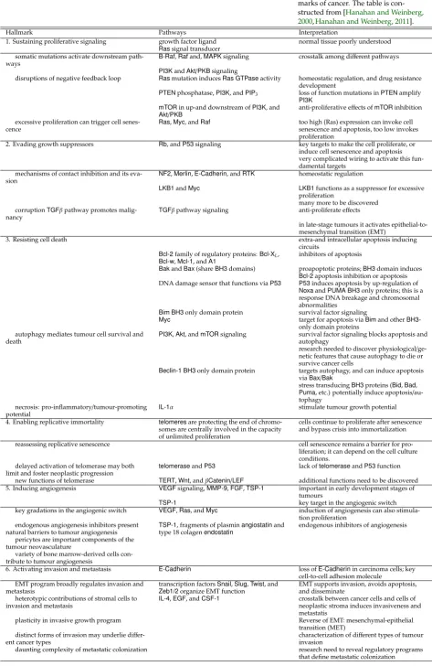
Figure1.5on page21pictures an overview of many fundamental biological interactions in cancer. Depending on the type, and sub-types of cancer, etc. different interactions have more importance for diagnosing and treating cancer in a more sophisticated approach. The following sections provide an overview of the most important known mechanisms in cancerous cells. Some of these mechanisms are explained in a frequently cited work: The hallmarks of cancer, it has been recently revised [Hanahan and Weinberg, 2000,Hanahan and Weinberg, 2011]. A hallmark can be defined as a feature of a system that differentiates it from other systems [Yuri, 2010]. These features will be introduced together with the corresponding biologi-cal implications. As a general guidance table1.2on page22provides a summary of the six hallmarks.

The following paragraphs will introduce the global statistics of cancer and fundamental cancer terminology. Some of these terms will reoccur in later chapters, other terms are fundamental for un-derstanding the literature.

Hallmark Pathways Interpretation

1. Sustaining proliferative signaling growth factor ligand normal tissue poorly understood

Rassignal transducer somatic mutations activate downstream

path-ways

B-Raf,Rafand,MAPKsignaling crosstalk among different pathways

PI3KandAkt/PKBsignaling

disruptions of negative feedback loop Rasmutation inducesRas GTPaseactivity homeostatic regulation, and drug resistance development

PTENphosphatase,PI3K, andPIP3 loss of function mutations inPTENamplify

PI3K mTORin up-and downstream ofPI3K, and

Akt/PKB

anti-proliferative effects ofmTORinhibition excessive proliferation can trigger cell

senes-cence

Ras,Myc, andRaf too high(Ras) expression can invoke cell senescence and apoptosis, too low invokes proliferation

2. Evading growth suppressors Rb, andP53signaling key targets to make the cell proliferate, or induce cell senescence and apoptosis very complicated wiring to activate this fun-damental targets

mechanisms of contact inhibition and its eva-sion

NF2,Merlin,E-Cadherin, andRTK homeostatic regulation

LKB1andMyc LKB1functions as a suppressor for excessive proliferation

many more to be discovered corruptionTGFβpathway promotes

malig-nancy

TGFβpathway signaling anti-proliferate effects

in late-stage tumours it activates epithelial-to-mesenchymal transition (EMT)

3. Resisting cell death extra-and intracellular apoptosis inducing circuits

Bcl-2family of regulatory proteins:Bcl-XL,

Bcl-w,Mcl-1, andA1

inhibitors of apoptosis

BakandBax(shareBH3domains) proapoptotic proteins;BH3domain induces

Bcl-2apoptosis inhibition or apoptosis DNA damage sensor that functions viaP53 P53induces apoptosis by up-regulation of

NoxaandPUMA BH3only proteins; this is a response DNA breakage and chromosomal abnormalities

Bim BH3only domain protein survival factor signaling

Myc target for apoptosis viaBimand otherBH3 -only domain proteins

autophagy mediates tumour cell survival and death

PI3K,Akt, andmTORsignaling survival factor signaling blocks apoptosis and autophagy

research needed to discover physiological/ ge-netic features that cause autophagy to die or survive cancer cells

Beclin-1 BH3only domain protein targets autophagy, and can induce apoptosis

viaBax/Bak

stress transducingBH3proteins (Bid,Bad,

Puma, etc.) potentially induce apoptosis/ au-tophagy

necrosis: pro-inflammatory/tumour-promoting potential

IL-1α stimulate tumour growth potential

4. Enabling replicative immortality telomeresare protecting the end of chromo-somes are centrally involved in the capacity of unlimited proliferation

cells continue to proliferate after senescence and bypass crisis into immortalization

reassessing replicative senescence cell senescence remains a barrier for pro-liferation; it can depend on the cell culture conditions.

delayed activation of telomerase may both limit and foster neoplastic progression

telomeraseandP53 lack oftelomeraseandP53function

new functions of telomerase TERT,Wnt, andβCatenin/LEF additional functions need to be discovered 5. Inducing angiogenesis VEGFsignaling,MMP-9,FGF,TSP-1 important in early development stages of

tumours

TSP-1 key target in the angiogenic switch

key gradations in the angiogenic switch VEGF,Ras, andMyc induction of angiogenesis can also stimula-tion proliferastimula-tion

endogenous angiogenesis inhibitors present natural barriers to tumour angiogenesis

TSP-1, fragments of plasminangiostatinand type 18 colagenendostatin

endogenous inhibitors of angiogenesis

pericytes are important components of the tumour neovasculature

variety of bone marrow-derived cells con-tribute to tumour angiogenesis

6. Activating invasion and metastasis E-Cadherin loss ofE-Cadherinin carcinoma cells; key cell-to-cell adhesion molecule

EMT program broadly regulates invasion and metastasis

transcription factorsSnail,Slug,Twist, and

Zeb1/2organize EMT function

EMT supports invasion, avoids apoptosis, and disseminate

heterotypic contributions of stromal cells to invasion and metastasis

IL-4,EGF, andCSF-1 crosstalk between cancer cells and cells of neoplastic stroma induces invasiveness and metastatis

plasticity in invasive growth program Reverse of EMT: mesenchymal-epithelial transition (MET)

distinct forms of invasion may underlie diff er-ent cancer types

characterization of different types of tumour invasion

Global statistics In global death statistics in the US [Murphy et al., 2012], EU [EUD, 2012], and UK [UKCR, 2012]diseases of heart (ICD:

I00-I09,I11,I13,I20-I51)8, andmalignant neoplasms (ICD: C00-C97)are 8_{ICD code is the International}

Classifi-cation of Disease coding system set by the World Health Organisation (WHO). the two main causes of death. Generally, diseases of the heart are

the main cause of death, whereas, e.g. in the UK people aged above 50 [UKCR, 2012], and in US for people aged between 45 and 64, more than 30 % died of cancer [Murphy et al., 2012].

Proliferation In many cancers proliferation is a driving force [Hall and Levison, 1990,Schlabach et al., 2008]. Proliferation leads to an increase of the number of cells, and therefore closely related to cell growth and division. Since the cell is a robust system, there are mechanisms that limit this proliferation [Albert et al., 2002,Hong et al., 2010]. One of this mechanisms is calledsenescence(i.e. aging of a biological organism), another mechanism is calledapoptosis(i.e cell death).

Differentiation Cell differentiation occurs when a cell in a multi-cellular organism is dedicated to become a specific cell type. The memory of the cellhas a predefined biological genetic footprint for each cell [Albert et al., 2002]. In tumour cells this footprint is disor-dered; the same genes are part of this footprint, but their expression levels differ from the prototype cell [Hong et al., 2010].

Metastasis A general capacity of malignant tumours is to spread into different organs, this capacity is calledmetastasis[Albert et al., 2002,Fidler, 2003,Hong et al., 2010]. Tumours that are formed in the original organ are calledprimary tumours. Analogously, tumours that are spread into a different organ are calledsecondary tumours. The transition of primary towards secondary tumour is often called colonization. E.g., a bone metastasis drug calledDenosumab (Pro-lia®by Amgen. Inc.), has been approved by the FDA for cancer pa-tients [Sethi and Kang, 2011].

Autophagy – angiogenesis Because of the proliferation and the spread of a tumour, a lot of energy is required to form a malig-nant tumour. There are two main energy related concepts active in tumour development: (1)autophagy(i.e. self-eating) [Kondo et al., 2005] and (2)angiogenesis(i.e. formation of new blood ves-sels) [Kalluri, 2003]. Both of these concepts can be seen as the re-quired energy to run the switch of the transition between benign towards malignant tumours.

Autophagy can suppress tumour growth, but at the same time it can stimulate tumour growth by providing new energy [Hippert et al., 2006]. The energy often comes from the inner cells of a tumour [Mathew et al., 2007]. Despite this dual role of autophagy, it also plays a role in drug resistance, e.g. in HER2+breast cancer treated with Herceptin (also called trastuzumab) autophagy markers were highly expressed [Vazquez-Martin et al., 2009].

() Angiogenesis, a term for the construction, repair, and migra-tion of blood vessels, is another fundamental biological program in cancer [Folkman, 1995,Kullari, 2003]. This program has been mainly seen as a switch for the transition from primary to secondary tumours. This switch runs when the angiogenic phenotypes are triggered. Since the mid 1990s there is growing evidence that an-giogenic tumour activity is fundamental for tumour growth and metastasis [Carmeliet, 2005,Sethi and Kang, 2011]. Recently, there has been multiple angiogenic inhibitors for the clinical practice, where side effects seem to be one of the biggest drawbacks. Since angiogenesis is a fundamental process in wound healing, heart func-tion, reproduction of vessels, etc. If a drug inhibits this process, it is shown to induce toxicity [Verheul and Pinedo, 2007]. In the clin-ical environment the progression-free survival was extended, as there was little improvement of the overall survival figures (e.g., pazopanib in renal cell cancer). More holistic drug that integrates multiple strategies into an agent might introduce less toxicity in the future.

Cell growth and division cycle An important biological process in cancer is the cell growth and division cycle [Hartwell and Kastan, 1994,Clyde et al., 2006]. The cell cycle is an ordered sequence of events whereby a cell grows and then divides resulting in the pro-duction of two daughter cells that are identical to the original parent cell.

The cell cycle may be considered in five separate phases [Albert et al., 2002]:

1. Gap one or G1 phase: the cell undergoes a series of biochemical and physiological changes including sustained growth.

3. Synthetic or S phase: the cell copies its DNA resulting in the development of duplicate copies of each chromosome.

4. Gap two or G2 phase: a second gap phase during which the proteins and complexes necessary for the remainder of the cell are synthesized.

5. Mitosis or M phase:mitosis, during which the cell divides with one set of chromosomes being allocated to each of the two result-ing daughter cells.

Cell regulation Cell regulation is essential for preserving the ap-propriate functionality of living cells and maintaining a healthy phenotype [Clyde, 2006]. Regulation is maintained through a vari-ety of gene expression processes which result in the supply of the proteins necessary for cell regulation at the correct time and in the correct quantities.

Cell regulation consists of a number of separate processes:

1. Growth and division cycle: this biological process occurs se-quentially in separate steps leading to a terminally differentiated adult cell.

2. Apoptopic pathways: this intrinsic and extrinsic process regu-lates cellular death at the appropriate time and to the appropriate extent.

3. Cell survival pathway and the anti-growth pathway: this pro-cess is important in maintaining the balance of cells essential for homeostasis in multi-cellular species. A collection of cellu-lar events, with an origin from different pathways, occur as a network.

4. Damage response pathways: this process monitors DNA dam-age and tries to repair DNA damdam-age. If damdam-age can not be re-paired, cell will go to apoptosis (see category2).

All these pathways link the cell’s internal processes. Specific parts of these pathways are also linked to external intervention processes. This can be illustrated by the action of growth factor, and other ligands which can direct appropriate cell regulation as well as other forms of interaction with adjacent cells, or the extra-cellular matrix can interact in the cell regulation process.

In the following sections, we describe important facts related breast- and ovarian cancer.

1.3.1

Breast cancer

Breast cancer is usually not difficult to diagnose. The problem lies with stratification of patients for the right treatment, because of intrinsic or acquired resistance to therapy is hard to predict. A more successful therapy for a specific patient is still an enormous scientific challenge because of theheterogenecityof cancer [Sorlie et al., 2001,Med, 2008].

Figure 1.6: Mammary ductal network (Modified from: [Med, 2008]). This ductal network is analysed to detect the stage of breast cancer.

Classification of breast cancer Breast cancer is one of the best under-stood cancers [Gray and Druker, 2012]. Breast carcinomas are not only classified upon their histopathological measurements, Sorlie et al [Sorlie et al., 2001] (see figure1.7on page27) illustrate, by ap-plying hierarchical clustering, that breast cancer can be classified according to the gene expressions of cDNA microarray experiments into three major groups:

1. ER+express typical protein of luminal epithelial cells.

• luminal subtype A (most frequently occurring breast cancer). • luminal subtype B (second most frequently occurring breast

cancer).

• luminal subtype C (least frequently occurring breast cancer).

2.

ER-• HER2+:ERBB2+.

This tumour occurs in approximately 20 % of all breast can-cers. HER2+tumours tend to be more aggressive than HER2-tumours [Azim and Jr., 2008]. Furthermore, these tumours are characterized with ErbB2 gene amplification and HER2 recep-tor overexpresssion [Yarden and Sliwkowski, 2001,Hynes and MacDonald, 2009].

• basal-like (15 % of all tumour carcinoma) • normal breast-like:

This type of carcinoma has been regarded as a different type [Sorlie et al., 2006]. Its analysis it very complicated since it is similar to epithelial cells; its histological characteristics and clinical prognosis are still under research.

Figure 1.7: Hierarchical clustering applied for the gene expression data (From Fig. 1 of Sorlie et al [Sorlie et al., 2001]).

B; they occur withERpositive,PRandHER2negative, andKi67

high.HER2breast cancer haveHER2positive,ERandPRnegative, andKi67high. It becomes more complicated for the triple negative breast cancers (ER,PR, andHER2negative andKi67high): basal-like.

For basal-like breast cancers are further subclassified [Rakha et al., 2008b]. Basal-like cancers can be identified with a positive expression of epidermal growth factor receptor (EGFR) and cytoker-atin 5/6 (CK 5/6) biomarkers [Cheang et al., 2006]. This classification is not perfect, since triple negative basal-like tumours appear with negative expressions ofEGFRandCK 5/6and not all basal-like tumour appear with triple-negative signature [Rakha et al., 2008a].

Finally,aprocrine typeareERandPRnegative and androgen re-ceptor (AR) is positively expressed [Celis et al., 2009]. It is not clear if this is a class of breast tumours is distinct because of clinicopatho-logical observations or can by part of any of the above described tumour classes [Gonzalez et al., 2008].

A systems approach could be beneficial to decipher the complex cascade of events that could further improve the treatment and management of breast cancer in the clinic [Barab ´asi and Oltai, 2004,

Nevins, 2007].

1.3.2

Ovarian cancer

Ovarian cancer is the fourth most common cancer death in the UK [UKCR, 2012], and the seventh most common cancer death in the US during 2008 [Jemal et al., 2011]. There are two main types of ovarian cancer: (1)epithelial ovarian cancer (EOC)and (2)ovarian germ cell tumour.

Epithelial ovarian cancer in early stage has a 5 year survival of ∼_{90 %, but for late stage it is}∼_{30 % [Lu et al., 2004,Faratian et al.,}

early detection of epithelial ovarian cancer [Lu et al., 2004,Tothill et al., 2008]. Despite a need for markers of early detection, a set of markers is needed to understand the underlying biological mecha-nisms and molecular pathogenesis to perform better diagnosis and prediction for epithelial ovarian cancer.

Ovarian germ cancer do not occur very often,∼_{1500 times in UK} during 2008 [Jemal et al., 2011], and they are treated different from epithelial ovarian cancers. Two main molecular markers exist to detect ovarian germ cancer: AFP(alpha-fetaprotein), andHCG (hu-man chorionic gonadotrophin). It appears mostly within younger women, and very often are completely cured.

Ovarian cancer has a lack of systems approaches for biomarker discovery and classification based on molecular pathology. These systems approaches have the potential to improve the treatment and management of ovarian cancer in the next decade. In breast cancer (see section1.3.1on page25), a set of biomarkers is well established into a clinical environment. The treatment of ovarian cancer could be improved by finding a similar set of biomarkers.

1.4

Application of systems approach in pathology

During the last decade, more and moresystemsapproaches have en-tered into the molecular biology field [Westerhoffand Palsson, 2004]. This systems approach is widely applied in engineering, software design, and other scientific fields [Hitchins, 2007]. The composi-tion of a system can be a colleccomposi-tion of different building blocks. Putting these building blocks together is often calledsynthesis, or a bottom-up approach. Alternatively, a system can be decomposed into smaller building blocks, also calledanalysis, or a top-down approach. Systems biology research can be seen as a pyramid of different building blocks (see figure1.8). Where the foundations of this pyramid are all the “omics” technologies available for data of genomes, exomes, proteomes, transcriptomes. metabolomes. On top of this “omics” technology, all “ology” disciplines help to formulate more holistic hypotheses of the system under investigation. These two bottom layers help to explain mechanisms that are important in ailments, drugs, and processes in life.

Traditional molecular biology research often happened with a bottom-up approach (reductionism), e.g. pathway analysis. Since more and more “omics” data is publicly available, more top-down approaches can be performed. System biology often occurs in hy-brid fashion, e.g. dynamical interactions between pathways are analysed to improve the understanding of cancer biology.

Systems biology becomes more and more the standard approach to perform research in drug discovery (i.e., during 2011: abiraterone, crizotinib, and vemurafenib) [Butcher et al., 2004,Garnett et al., 2012], bio-marker selection (i.e.,ER,PR,HER2, andKi67for breast cancer) [van’t Veer et al., 2005,Faratian and Bartlett, 2008,Faratian et al., 2011], understanding biological mechanisms(i.e., C35 gene expression to indicate tumour invasion) [Faratian et al., 2009].

Reverse engineering [Csete and Doyle, 2002] is a strategy to re-design functionality of an existing system. In software engineering,

it is used to obtain the source code from the object code9of a pro- 9_{The object code is the machine code}

that hardware needs to execute a program.

gram. In systems biology, this term is often used for specific compu-tational techniques applied on “omics” data, e.g. automated reverse engineering ordinary differential equations (ODE) [Bongard and Lipson, 2007], Bayesian networks [Hartemink, 2005], etc.

To conclude this first chapter, a systems approach can enrich con-clusions in biology and pathology. This systems approach helps to discover an “omics” footprint of a category of a biological process. This footprint aids to understand the mechanisms of this biologi-cal process, and therefore can potentially improve the insights of the heterogeneity; this is required to be able to make more holistic developments that can potentially contribute towards, e.g. a more personalized diagnosis and treatment [Cesario and Marcus, 2011]. The future of systems approaches will require new integrated approaches to examine fairly complex and heterogeneous data sets, e.g. expression data, sequence information, functional annotation, and the literature. Not only data complexity is a major challenge;

the growth of sequencing data is beating Moore’s law10in 2008 10_{Moore’s law is used in computer}

hardware design. It defines that the amount of transistors on integrated circuits doubles every two years. [Goldman and Yang, 2008]. As a consequence of this growth, the

rate of the cost per genome decreases faster as the rate of the cost per byte in 2008.

1.5

Layout of the thesis

In the next four chapters, I will first guide you through the method-ologies I applied during this research: machine learning techniques and “-omics” technologies. Mainly, I worked on engineering bioin-formatics tools that could explain fundamental pathological pro-cesses. This novel computational tools are an important facet in the interpretation of heterogeneous data collected with state-of-the-art technologies.

This doctorate is the result of research in two important facets of pathology: (1) biomaker discovery and (2) tumour invasion.

Biomarker discovery The biomarker discovery study is performed for ovarian carcinoma. The data of the Edinburgh Ovarian Cancer Register is used to investigate candidate proteome biomarkers for prognosis. The characterization of the predictability of more tradi-tional clinicopathological measurements and a proteomics profile for prognosis determination is analysed with novel engineered com-putational tools. The results of these new constructed bioinformatic tools are presented in chapter3.

These bioinformatics tools were capable to quantify the signif-icance of the set of biomarkers and classify patients if they have a high- or low risk of one-year progression-free and three-year overall survival. Furthermore, I was able to collect a validation data set for an independent group of patients. This allowed me to have hand-on laboratory experience together with the application of high-quality imaging analysis technology. The performance of these computa-tional models after cross-validation and the separate validation data set are at the moment of writing the best found in the literature.

These state-of-the-art bioinformatics tools are also used to con-struct a biological signature for the histopathological assemblies of the data set. Potentially, they can be applied in many different aspects, e.g. for the validation of various biomarkers in a clinical practice, support engineering of new biomarkers, etc.

The results and the computational methodologies are presented in chapter3.

Tumour invasion Tumour invasion assays are extremely heteroge-neous and pathological characterization of their morphology is im-portant and poorly quantified [Katz et al., 2011]. This tumour inva-sion study is concentrated on the morphological characterization of tumours. The data collected by collaborators applied state-of-the-art imaging analysis for the collection of morphological measurements that are known to be important for histopathological examination.

Choice of methodology

Modernism and

postmodernism might be characterised as the two major forces of philosophical thought that have influenced and continue to influence the changes in thinking in research methods. Modernism is associated with the

scientific understanding of truth and knowledge, claiming that there is one ultimate, objective truth; and postmodernism relates to the human-centred holistic perspective, maintaining that there are subjective, multiple truths.

Webster, L. and Mertova, P

The first part of this chapter introduces the computational method-ologies used during this PhD. As presented in the first chapter, I will start with the main generative machine learning approach applied: Bayesian networks. Bayesian networks applied to performstructure learningwill be explained. This will be followed by the discrimina-tive machine learning algorithms, i.e. the traditionallinear models andsupport vector machines (SVMs). The final computational ap-proach explained in this chapter issurvival analysis. This first part will end with the discussion of different machine learning strategies used for the validation of the resulting models.

The second part of this chapter will describe the biological exper-iments applied in the course of this PhD.Reverse phase protein arrays (RPPA)and thetissue microarrays (TMA)experiments will be de-scribed. I applied TMA technology, in association with collaborators of the Division of Pathology at the University of Edinburgh, for the collection of a validation data set for proteome biomarker validation (see chapter3).

performed Bayesian network analysis to build computational mod-els. In consultation with my supervisors, I have proposed to work with various computational modelling techniques; this techniques are nowadays called machine learning. Machine learning has been applied previously in Bioinformatics [Baldi and Brunak, 2001].

2.1

Computational methodologies

Systems approaches in pathology require computational modelling to quantify their data resources. Since cancer is such a complicated collection of diseases, mathematical modelling aids to understand the underlying patterns. This mathematical modelling is extremely challenging and the predictive capacity inferred form biological data is not always sufficient to construct high quality models [Roberts et al., 2012]. What is modelling and where does a model stands for? A quote of Einstein gives a very good starting point for a usable model:

"Everything should be made as simple as possible but not simpler".

This applies also to a model, a useful model models a sufficient amount of complexity in as simple as possible way.

In computational modelling one could distinguish two different approaches:

1. Process-driven approach:

• The model is constructed from assumptions, expert knowl-edge, literature, etc.. The process behind the model is de-scribed.

• Predictions can be made based onexpert knowledge.

• Examples of process-driven computational approaches are or-dinary differential equations (ODEs), inference over a Bayesian network, etc.

2. Data-driven approach:

• The data is used as the driving-force behind the construction of the model. The model is inferred from experimental data. • Predictions are made fromexperimental data.

• Examples of data-driven computational approaches are linear models, support vector machines, structure learning with Bayesian networks, etc.

In reality process-driven and data-driven approaches are often combined. Combining knowledge from earlier biological research with data from current experiments is a common strategy in compu-tational modelling.