S
c
h
o
o
l
o
f
E
c
o
n
o
m
ic
s
&
F
in
a
n
c
e
D
is
c
u
s
s
io
n
P
a
p
e
r
s
School of Economics & Finance
Partial Knowledge Restrictions on
the Two-Stage Threshold Model of
Choice
Paola Manzini, Marco Mariotti and Christopher J. Tyson
School of Economics and Finance Discussion Paper No. 1503 5 Mar 2015
Partial Knowledge Restrictions on the
Two-Stage Threshold Model of Choice
Paola Manzini
∗Marco Mariotti
†Christopher J. Tyson
‡February 10, 2015
Abstract
In the context of the two-stage threshold model of decision making, with the agent’s choices determined by the interaction of three “struc-tural variables,” we study the restrictions on behavior that arise when one or more variables are exogenously known. Our results supply nec-essary and sufficient conditions for consistency with the model for all possible states of partial knowledge, and for both single- and multi-valued choice functions.
1
Introduction
Recent work in the theory of individual choice behavior has modified the classical preference maximization hypothesis in various ways. One approach has been to weaken the consistency properties that preferences are ordinarily assumed to possess.1 Another has been to study relationships between
pref-erence and choice other than straightforward maximization.2 And a third has
been to permit additional, non-preference-related factors—as well as multiple preferences—to influence decision making in some way.3
∗University of St. Andrews and IZA, Bonn. Email: [[email protected]]. †Queen Mary University of London. Email: [[email protected]].
‡Queen Mary University of London. Email: [[email protected]].
1
For example, Eliaz and Ok [9], Mandler [14], Nishimura and Ok [23], and others allow preferences to be incomplete (following in the tradition of Aumann [2] and Bewley [5]).
2
Models of this sort have been axiomatized by Baigent and Gaertner [3], Eliaz et al. [10], Mariotti [19], and Tyson [30], among others.
3
Under the last of the three approaches just listed, the revealed preference exercise required to characterize a given model can be quite complex, since multiple factors must be inferred simultaneously from behavior. Moreover, models with more than one component make possible a variant of the usual characterization problem: An outside observer can test a collection of choice data for consistency with the model while treating one or more components as known.
For example, suppose that we postulate a decision maker who maximizes a utility function over the alternatives that he or she notices, but pays attention only to those options with a sufficiently high level of salience (with regard to the visual or another sensory system). If salience is directly measurable, then the relevant question is whether these measurements and the choice data to-gether can be reconciled with our behavioral hypothesis.4 And this means, of
course, finding suitable assignments of the unobserved components—namely, the utility function and the salience thresholds.
As another example, imagine a choice among lotteries by a satisficing agent who decides between the options deemed satisfactory by following a social-norm ordering. On the one hand, the social norm might be known to the theorist, in which case it and the choice data must be jointly reconciled with the model by specifying the utilities and satisficing thresholds. Alterna-tively, perhaps the norm is unknown but we wish to introduce a maintained assumption of risk neutrality. In the latter case our search will be for satis-ficing thresholds (relative to expected value) plus a social norm that together generate the observed behavior.
Evidently, questions of this sort can be posed for any multiple-component model of choice, with any subset of the components taken to be known. In an electoral setting we might plausibly know the economic interests of a voter but not his or her ideology, while in a managerial setting we might assume profit maximization subject to an unobserved market-share constraint. Note that a model component could be designated as “known” due to an assump-tion, a physical observaassump-tion, econometric estimates from a separate data set, or background knowledge of the agent’s environment, among other reasons.
In this paper we explore the issue of testing model consistency under partial knowledge—one that appears to be largely unexamined in the context of axiomatic choice theory. To give this enterprise some concreteness, we shall commit to a particular model of how choices are determined by the
Cherepanov et al. [8], and Masatlioglu and Nakajima [20] on search and consideration sets; and Mandler et al. [15], Manzini and Mariotti [17], and Bajraj and ¨Ulk¨u [4] on procedural models.
4
interaction of various factors. We adopt a framework that is deliberately very general, and can accommodate the examples mentioned above. For each menuAof alternatives, the “two-stage threshold” (TST) model of choice specifies that the agent will select an option that solves
max
x∈A g(x) subject to f(x)≥θ(A). (1)
Here the model components, which we shall call “structural variables,” are real-valued functions f and g defined on the space of alternatives, plus a real-valued function θ defined on the space of menus.
The TST framework has no fixed interpretation. Indeed, the model over-laps with several existing theories based on very different hypotheses about the process of decision making. One possibility is to interpretf as a measure of consideration or attention priority, θ as a cognition-threshold map, and g
as a utility function; as in the contributions of Lleras et al. [13] and Masatli-oglu et al. [21].5 Another possibility is to interpret f as the utility function, θ as a utility-threshold map, and g as a salience measure; as in Tyson [31]. Under these two interpretations the first stage of the model captures, respec-tively, the “consideration set” (a concept from the marketing literature) and Simon’s [27] notion of satisficing.6
In its general form the TST model has been characterized by Manzini et al. [18], who demonstrate that Equation 1 can accommodate a wide range of behavior patterns. Indeed, when each set of acceptable choices is required to be a singleton, it is straightforward to show that any observed data set can be generated by the model (see Proposition 2.6). Moreover, even if we allow multiple acceptable choices, the constraints imposed by the framework itself remain weak (see Theorem 2.5). While the theories mentioned above reduce this freedom by imposing specialized restrictions on the structural variables, our approach will be to fix one or more variables completely and leave the others entirely unconstrained.7 We then seek to identify the forms
of behavior that remain consistent with the model.
Given a particular interpretation of the model, some structural variables will be more naturally assumed to be known than others. Since our intention is to avoid favoring any specific viewpoint, we provide a complete and hence interpretation-free collection of characterization results: For any strict subset of the three structural variables, we supply necessary and sufficient conditions for behavior to be compatible with the TST model when the variables in the
5
Related models are studied by Eliaz and Spiegler [11] and Spears [28].
6
For further details of these interpretations of the TST framework, see [18, pp. 879–881].
7
subset are known and all others are unrestricted.8 This collection of results—
together with posing the partial knowledge question for multiple-component choice models—makes up the contribution of the paper.
Broadly speaking, our analytical method is to use the choice data together with the known variables to infer as much information as we can about the unobserved variables. We then look for ways in which this information could be self-contradictory, and formulate axioms that rule them out. Such axioms will always be necessary for behavior to be compatible with the model. And if our search for contradictions is thorough enough, they will also be sufficient (though demonstrating this may require extended arguments).
For example, suppose thatg is known while bothf and θ are unobserved (cf. Theorem 4.7). If alternatives x and y are both on menu A, and if also
g(x) > g(y), then clearly x and y cannot both be chosen from A. This is the simplest illustration of how choice data and a known structural variable together can lead to a contradiction, which must be ruled out axiomatically. Suppose now that f and g are both known, with only θ unobserved (cf. Theorem 4.8). Since g is known, the variety of contradiction seen in the preceding paragraph must still be avoided. Furthermore, if alternatives
x and y are both on menuA, and if also f(x)≥f(y) and g(x)≥g(y), then we cannot have that y is chosen from A unless x too is chosen. These two types of contradictions turn out to exhaust the implications of the model when both f and g are known, which is to say that axioms ruling them out provide the desired characterization.
The remainder of the paper is structured as follows. Section 2 defines the TST framework and reviews the axiomatization of the unconstrained model given by Manzini et al. [18]. Our novel results are stated first in Section 3 for the special case of single-valued choice, and then in Section 4 for the multi-valued case. Section 5 contains a brief concluding discussion. Proofs of the general (i.e., multi-valued) versions of our results can be found in the Appendix.
8
We assume that knowledge of one structural variable has no direct implications for the unknown variables, which can be chosen arbitrarily to generate the observed behavior. This assumption will not hold under interpretations of the model that motivate joint restrictions on the variables. For example, in [31] the functions f and θ are linked by the property of “expansiveness.” It is even possible that knowledge of one variable could completely determine another, for instance if θ(A) equals the average|A|−1P
x∈Af(x) of
2
The two-stage threshold model
LetX be a nonempty, finite set, and letD ⊆ A= 2X \ {∅}. The elements of
X are called alternatives, the elements of D are called menus, and any map
C :D → Asuch that ∀A∈ D we have C(A)⊆A is called achoice function. The choice set C(A) contains the alternatives that are chosen from menu
A. A choice function is single-valued if it returns only singleton choice sets. Without loss of generality, we shall assume that ∀x∈X we have {x} ∈ D.
In the TST model, the choice set associated with menu A is constructed by maximizing g(x) subject to f(x)≥θ(A). Here f :X → ℜ is theprimary criterion, g : X → ℜ the secondary criterion, and θ : D → ℜ the threshold map. These three components of the model are termed structural variables, any triple hf, θ, gi is a profile, and any pair hf, θiis a primary profile.
Given a primary profilehf, θi and an A∈ D, write Γ(A|f, θ) ={x∈ A:
f(x)≥θ(A)}for the subset of available alternatives whose primary criterion values are above the relevant threshold. The TST model can now be defined formally as follows.
2.1 Definition. Atwo-stage threshold representation ofCis a profilehf, θ, gi
such that ∀A∈ D we have C(A) = argmaxx∈Γ(A|f,θ)g(x).
In order to axiomatize this model, Manzini et al. [18] use several binary relations that are revealed by the agent’s choices. The separation relation
encodes situations where one alternative is chosen and a second (available) alternative is rejected.
2.2 Definition. Let xSy if ∃A∈ D such that x∈C(A) and y∈A\C(A).
The togetherness relation encodes situations where two alternatives both are chosen, and its transitive closure is the extended togetherness relation.9
2.3 Definition. Let xT y if ∃A ∈ D such that x, y ∈ C(A), and let xEy if
∃z1, z2, . . . , zn ∈X such that x=z1T z2T · · ·T zn =y.
Finally, the first-stage separation relation encodes separations that must be attributed to the primary criterion, since an extended togetherness relation-ship guarantees equal values of the secondary criterion.10
2.4 Definition. Let xF y if xEy and xSy.
9
Recall that a relationRis transitive ifxRyRz⇒xRz, and that the transitive closure ofR is the smallest transitive relation containing it.
10
More explicitly, if xEy then x =z1T z2T· · ·T zn = y, which under the TST model
implies thatg(x) =g(z1) =g(z2) =· · ·=g(zn) =g(y) for somez1, z2, . . . , zn∈X. If also
Manzini et al. [18, pp. 876–879] prove that acyclicity of this last relation is the one and only condition needed to characterize the TST model in the absence of known structural variables.11
2.5 Theorem. A choice function has a two-stage threshold representation if and only if the relation F is acyclic.
Moreover, since the relations T, E, andF are all empty in the single-valued case, here the acyclicity condition holds trivially and so consistency with the model is assured.
2.6 Proposition. Any single-valued choice function has a two-stage thresh-old representation.
3
Single-valued choice
3.1
One known variable
We study partial knowledge restrictions on the TST model first under the simplifying assumption of single-valued choice, and considering situations where just one of the three structural variables is known. As we shall see, even this minimal type of partial knowledge restriction gives empirical content to a framework that, as shown in Proposition 2.6, is otherwise vacuous: In each situation with one known variable the model can be characterized by an acyclicity condition like that employed in Theorem 2.5.
Known primary criterion. Suppose that the primary criterion f is known, while the threshold mapθ and secondary criteriongare not, and letx, y ∈A. In this case knowledge thatf(y)≥f(x) implies thatysurvives the first stage of choice from A if x does so; i.e., that x ∈Γ(A|f, θ) ⇒ y ∈Γ(A|f, θ). But then from the observationxSywe can deduce thatg(x)> g(y), sincexandy
must have been separated at the second stage. In other words, second-stage superiority of one alternative over another is revealed by the relation defined as follows in terms of the known f and observed C.
3.1 Definition. Let xHfy if f(y)≥f(x) and xSy.
SinceHf impliesstrict second-stage superiority between alternatives, this
relation must be acyclic for the model to hold. That is to say, acyclicity ofHf
is necessary forC to admit a TST representation consistent with the partial profile hf,·,·i.
11
3.2 Example. Letf(x) =f(y) = 1,C(xy) =x, and C(xyz) = y. Ifhf, θ, gi
were a TST representation of C, then f(y)≥ f(x) and C(xy) = x together would imply g(x)> g(y), but at the same time f(x)≥f(y) and C(xyz) = y
would imply g(y)> g(x), a contradiction.
Our first partial-knowledge result for the TST model states that acyclicity of Hf is sufficient as well as necessary, and thus characterizes the situation
in question.12
3.3 Proposition. A single-valued choice function has a two-stage threshold representation consistent with hf,·,·i if and only if Hf is acyclic.
Observe that once we have acyclicity of Hf, which is needed to construct a
suitable revealed secondary criterion, no further axiom is required to ensure the existence of an appropriate threshold map—this comes “for free.”
Known secondary criterion. Now suppose that it is the secondary criterion
g that is known, so that our task is to construct the primary profile. Here the first-stage separation relation used in Theorem 2.5 is unhelpful (since it is always empty in the single-valued case), but we can use our knowledge of
g to define a new revealed relation that performs the same role.
3.4 Definition. Let xHgy if bothg(y)≥g(x) and xSy.
3.5 Proposition. A single-valued choice function has a two-stage threshold representation consistent with h·,·, gi if and only if Hg is acyclic.
Somewhat surprisingly, both the definitions ofHf and Hg and the associated
characterization results are exactly parallel, even though the two stages of the TST model are not in any sense interchangeable.
Known threshold map. Next we consider the possibility of a known threshold mapθ. In this situation if we can findA, B ∈ Dandy ∈A∩B such thaty∈
C(B) and θ(B) ≥ θ(A), then clearly we can conclude that f(y) ≥ θ(A). If moreover both x∈C(A) andy /∈C(A) (noting that under single-valuedness the latter is immediate for y6=x), theny must have been eliminated fromA
at the second stage and hence we must have g(x)> g(y).
To capture this method of deducing second-stage superiority from the known θ and observed C, we define thecritical threshold for alternativey.
3.6 Definition. Let M(y|θ) = max{θ(A) :A∈ D ∧y∈C(A)}.
12
In other words, the critical threshold is the highest threshold of any menu to whose choice set the alternative belongs, with the obvious consequence that
y ∈C(A)⇒M(y|θ)≥θ(A).13 The argument above is then expressed in the
construction of the following revealed relation.
3.7 Definition. Let xHθy if ∃A ∈ D such that M(y|θ)≥ θ(A), x ∈ C(A),
and y ∈A\C(A).
Once again our characterization imposes acyclicity, and no additional axioms are needed.
3.8 Proposition. A single-valued choice function has a two-stage threshold representation consistent with h·, θ,·i if and only if Hθ is acyclic.
3.2
Two known variables
To complete our analysis of single-valued choice functions, we proceed to axiomatize the TST model in situations where two of the structural variables are known.
Known secondary criterion plus one primary variable. When both criteria are known, the assertion xHfy continues to imply that g(x) > g(y). But
instead of merely being checked for cycles, as in Proposition 3.3, inequalities of this sort can now be tested directly against the observed g.
3.9 Example. Letf(x) = 1, f(y) = 2, g(x) =g(y) = 0, and C(xy) =x. If
hf, θ, gi were a TST representation of C, then f(y) ≥ f(x) and C(xy) = x
together would imply g(x)> g(y), which is known to be false.
Our result for this situation states that consistency of deduced and observed second-stage superiority is precisely what is needed for the desired charac-terization.
3.10 Proposition. A single-valued choice function has a two-stage threshold representation consistent with hf,·, gi if and only if xHfy⇒g(x)> g(y).
In a similar way, our axiom for the case of known θ can be adapted to characterize the case of knownθ andg. Instead of checking the revealed rela-tion Hθ for cycles, we simply test it against the observed secondary criterion.
3.11 Proposition. A single-valued choice function has a two-stage threshold representation consistent with h·, θ, gi if and only if xHθy⇒g(x)> g(y).
13
Known primary profile. Finally, consider a situation in which the full primary profilehf, θiis known. Sincef is known, the conditionM(y|θ)≥θ(A) in the definition of Hθ (which guarantees that y survives the first stage of choice
from menu A) can be replaced with a direct assumption that f(y) ≥ θ(A). This modification leads to the following revealed relation, which continues to encode second-stage superiority.
3.12 Definition. Let xHf θy if ∃A ∈ D such that f(y) ≥ θ(A), x ∈ C(A),
and y ∈A\C(A).
As might be expected, our new relation must be acyclic if C is to admit a TST representation. This acyclicity is not sufficient, however, because it is also possible for the known hf, θi and the observed C to contradict each other outright—in a way that has nothing to do with inferences about the second stage.
3.13 Example. Let f(x) = 1, f(y) = 3, θ(xyz) = 2, and C(xyz) = x. If
hf, θ, gi were a TST representation of C, thenx∈C(xyz) would imply that
f(x)≥θ(xyz), which is known to be false.
The additional axiom required says simply that alternatives in the choice set assigned to Acan have primary criterion values no smaller thanθ(A).14 Our
characterization result for the present case therefore appears as follows.
3.14 Proposition. A single-valued choice function has a two-stage thresh-old representation consistent with hf, θ,·i if and only if Hf θ is acyclic and
f[C(A)]≥θ(A).
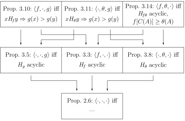
Our axiomatizations of the TST model with partial knowledge and single-valued choice are summarized in Figure 1, which also shows the logical rela-tionships among these results. For example, starting from Proposition 3.10, we can discard our knowledge of g and thereby arrive at Proposition 3.3. Hence any choice function covered by the former result must be covered by the latter (as well as by Proposition 3.5, since we can discard our knowledge of f).15 While our axioms will need to be generalized appropriately to deal
with the multi-valued case, these logical relationships will remain intact.
14
In other words,∀x∈C(A) we havef(x)≥θ(A); an assertion that we shall abbreviate as f[C(A)]≥θ(A).
15
Prop. 2.6: h·,·,·i iff —
❄
❄ ❄
Prop. 3.5: h·,·, gi iff
Hg acyclic
Prop. 3.3: hf,·,·iiff
Hf acyclic
Prop. 3.8: h·, θ,·i iff
Hθ acyclic
Prop. 3.10: hf,·, giiff
xHfy⇒g(x)> g(y)
Prop. 3.11: h·, θ, gi iff
xHθy⇒g(x)> g(y)
Prop. 3.14: hf, θ,·i iff
Hf θ acyclic,
f[C(A)]≥θ(A)
[image:11.595.117.479.126.362.2]❄ ❄ ❄ ❄ ❄ ❄
Figure 1: Summary of characterization results for single-valued choice.
4
Multi-valued choice
4.1
Preliminary comments
While useful and intuitive, the results in Section 3 are insufficient for a com-plete understanding of TST representations with known structural variables. This is because the maintained assumption of single-valued choice substan-tially limits the scope of the theory and—as we shall argue below—has no fully satisfactory justification in the present context. On the contrary, there are good reasons here to prefer results derived in a multi-valued setting.
One reason is that the standard theory of utility maximization requires multi-valued choice in order to allow for indifference. The supposedly more flexible TST framework should be a true generalization of the standard the-ory, and for this an extension to the multi-valued environment is needed. A related point is that under the consideration-set interpretation of the TST model (see Section 1), it is desirable to avoid imposing a no-indifference as-sumption on the agent’s utility function g.
always reduces the menu to a single alternative, then of course all later phases become irrelevant. Thus if we routinely study choice procedures under the assumption of single-valuedness, then we cannot meaningfully embed them in a multi-stage model.
4.2
One known variable
We proceed now to generalize Propositions 3.3, 3.5, and 3.8 to the multi-valued setting.
One known primary variable. Whenf is known, the relationHf continues to
reveal second-stage superiority. But in the multi-valued case alternatives can also be related by E, which is easily seen to reveal second-stage indifference. Choice data can thus be incompatible with the TST model even when there is no Hf-cycle, as seen in the following example.
4.1 Example. Letf(x) = 1,f(y) = 2,f(z) = 0,C(xy) = x,C(xz) =z, and
C(yz) = yz. If hf, θ, gi were a TST representation of C, then f(y) ≥ f(x) and C(xy) =x together would imply g(x)> g(y), and likewise f(x) ≥f(z) and C(xz) = z would imply g(z)> g(x). But then C(yz) = yz would imply
g(y) = g(z)> g(x)> g(y), a contradiction.
The choice function in this example hasF empty (and therefore vacuously acyclic), so there is no difficulty in exhibiting a TST representation when all three structural variables are free. It is only in combination with the specified
f that C conflicts with the model, due to the mixed cycle yEzHfxHfy.
With such cases in mind, we define formally the relation of being linked by a chain of alternatives connected sequentially by either Hf or E.
4.2 Definition. Let xWfy if ∃z1, z2, . . . , zn ∈ X such that z1 = x, zn = y,
and for each k ∈ {1,2, . . . , n−1} we have either zkHfzk+1 orzkEzk+1.
This relation reveals weak second-stage superiority, and strict superiority if at least one link in the chain is viaHf. The condition needed for a
character-ization, analogous to Richter’s [24, p. 637] Congruence axiom, is then that no alternative bear Wf to itself except via extended togetherness.
4.3 Theorem. A choice function has a two-stage threshold representation consistent with hf,·,·i if and only if xWfy ⇒ ¬[yHfx].
The case of a known θ can be handled similarly. Here Hθ reveals strict
4.4 Definition. Let xWθy if ∃z1, z2, . . . , zn ∈ X such that z1 = x, zn = y,
and for each k ∈ {1,2, . . . , n−1} we have either zkHθzk+1 orzkEzk+1.
Our result then uses a Congruence-like condition to identify the data sets consistent with the model.
4.5 Theorem. A choice function has a two-stage threshold representation consistent with h·, θ,·i if and only if xWθy ⇒ ¬[yHθx].
Known secondary criterion. Wheng is the known variable, it remains true in the multi-valued case thatHg must be acyclic. But since this relation reveals
first-stage superiority, combining it with extended togetherness is unhelpful. Instead, we need to check that revealed second-stage indifference agrees with the observed secondary criterion, which is to say that alternatives related by
E have identical g-values.
4.6 Example. Let g(x) = 1, g(y) = 2, C(xz) = xz, and C(xyz) = yz. If
hf, θ, gi were a TST representation ofC, thenC(xz) =xz would imply that
g(x) =g(z), whileC(xyz) =yz would imply that g(z) =g(y). But then we would have g(x) =g(y), which is known to be false.
4.7 Theorem. A choice function has a two-stage threshold representation consistent with h·,·, gi if and only if Hg is acyclic and xEy⇒g(x) =g(y).
4.3
Two known variables
Finally, we develop multi-valued versions of Propositions 3.10, 3.11, and 3.14.
Known secondary criterion plus one primary variable. When the primary and secondary criteria are both known, we must again test revealed second-stage indifference for consistency with the observedg. This test may be conducted independently from the consistency check on Hf used in Proposition 3.10,
resulting in the following characterization.
4.8 Theorem. A choice function has a two-stage threshold representation consistent withhf,·, giif and only ifxHfy⇒g(x)> g(y)andxEy⇒g(x) =
g(y).
Conveniently, the same straightforward modification also succeeds in the case of known g together with θ.
4.9 Theorem. A choice function has a two-stage threshold representation consistent withh·, θ, giif and only ifxHθy⇒g(x)> g(y)andxEy⇒g(x) =
Known primary profile. When the first-stage structural variables are both known, weak second-stage superiority is revealed by the following relation.
4.10 Definition. LetxWf θy if ∃z1, z2, . . . , zn∈X such thatz1 =x, zn=y,
and for each k ∈ {1,2, . . . , n−1} we have either zkHf θzk+1 orzkEzk+1.
As in Theorems 4.3 and 4.5, we can use this relation to strengthen the re-quirement thatHf θbe acyclic. In combination with the condition that chosen
alternatives survive the (fully observable) first stage, this strengthened axiom achieves our final characterization.16
4.11 Theorem. A choice function has a two-stage threshold representation consistent withhf, θ,·iif and only ifxWf θy⇒ ¬[yHf θx]andf[C(A)]≥θ(A).
Our axiomatizations with partial knowledge and multi-valued choice are summarized in Figure 2. As anticipated in the discussion of Figure 1 above, the conditions used when two structural variables are known together imply those used when each is known separately (which are in turn always stronger than the condition needed when all three variables are free). Moreover, it is not difficult to confirm that each single-valued characterization in Section 3 is a corollary of the corresponding multi-valued result.17
5
Discussion
The axiomatizations summarized in Figures 1 and 2 constitute a complete analysis of choice under partial knowledge in the context of the two-stage threshold model. Our results involve a number of acyclicity and Congruence-like conditions similar to those used in traditional choice theory, as well as other conditions with fewer precedents in the literature.
In addition to establishing these specific results, a secondary goal of the paper has been to introduce the issue of partial knowledge itself. Outside of the TST context, partial-knowledge characterizations can be developed for choice-theoretic models that include different “structural variables.” If the
16
Unlike Theorems 4.3 and 4.5, Theorem 4.11 can be viewed as a direct consequence of Richter’s [24] classical axiomatization. This is because when the entire primary profile is observable, the subsets Γ(A|f, θ) of alternatives that survive the first stage are themselves observable. Providedf[C(A)]≥θ(A), these survivor subsets can be treated as surrogate menus, and the TST characterization problem reduces to the classical exercise. (The same is true, mutatis mutandis, for Proposition 3.14.)
17
For example, under single-valued choice we have thatEis empty,Wf is the transitive
closure ofHf, and the condition thatxWfy⇒ ¬[yHfx] (used in Theorem 4.3) amounts to
Thm 2.5: h·,·,·iiff
F acyclic
❄
❄ ❄
Thm 4.7: h·,·, gi iff
Hg acyclic,
xEy⇒g(x) =g(y)
Thm 4.3: hf,·,·i iff
xWfy⇒ ¬[yHfx]
Thm 4.5: h·, θ,·i iff
xWθy⇒ ¬[yHθx]
Thm 4.8: hf,·, giiff
xHfy⇒g(x)> g(y),
xEy⇒g(x) =g(y)
Thm 4.9: h·, θ, giiff
xHθy ⇒g(x)> g(y),
xEy⇒g(x) =g(y)
Thm 4.11: hf, θ,·iiff
xWf θy⇒ ¬[yHf θx],
f[C(A)]≥θ(A)
[image:15.595.117.479.126.363.2]❄ ❄ ❄ ❄ ❄ ❄
Figure 2: Summary of characterization results for multi-valued choice.
models have features in common with the present framework—such as mul-tiple stages or threshold effects—then it may be hoped that our techniques will be transferable to some degree to these new settings.
For example, consider the following variant of the “rational shortlist method” (RSM) model proposed by Manzini and Mariotti [16]. In the first of two stages, the decision maker eliminates any alternative that is not max-imal with respect to an asymmetric binary relation≻.18 Then, in the second
stage, a criterion function g is optimized in the usual way. Since maximiza-tion over menu A of an asymmetric≻cannot in general be represented with a threshold structure Γ(A|f, θ), this model is not covered by the TST frame-work. Moreover, since optimization of a secondary criterion is stronger than the second-stage procedure specified by Manzini and Mariotti, the new model is a special case of an RSM.
The model described above would place restrictions on behavior even under single-valued choice.19 Furthermore, we might wonder whatadditional
restrictions are implied by knowledge of either≻org. Assuming a known ≻
would lead to a situation very similar to that in Theorem 4.11, whose proof can be suitably modified (see Footnote 16). Alternatively, assuming a known
18
Recall that a relationRis asymmetric ifxRy⇒ ¬[yRx].
19
g would lead to a situation resembling that in Theorem 4.7, and one that poses more of a challenge. Here the objective would be to use the known g
and the observed C together to infer information about the unknown≻, and to assemble a set of axioms that rules out all possible contradictions.20
Another setting in which partial knowledge restrictions could be studied is that of Salant and Rubinstein’s [26] “salient consideration functions.” Here choice sets have the structure C(A) =Sni=1{x∈A :∀y ∈A¬[yPix]}, where
n is a natural number and each Pi is a relation. Apart from the constraints
intrinsic to this model, we can ask what additional behavioral restrictions are implied by knowledge ofn, or of one or more of thePi relations. And similar
questions can be posed in the setting of Kalai et al.’s [12] “rationalization by multiple rationales,” another prominent multiple-factor model of choice.
A
Appendix
As illustrated in Figures 1 and 2, results for TST representations with more known variables can be used to help prove results with less known variables. For example, to demonstrate that the conditions in Theorem 4.7 are sufficient for a representation consistent with h·,·, gi, it is enough to define a primary criterion f such that the conditions in Theorem 4.8 hold.
We shall make good use of this proof strategy, and so in order to preserve a sequential logical progression we shall prove our characterization results non-consecutively. Specifically, we prove first Theorem 4.8, followed by The-orems 4.3 and 4.7. We then prove Theorem 4.11, followed by Theorem 4.5. And lastly we prove Theorem 4.9.
A few items of notation not employed in the main text will be used in the proofs: We writexR∗yif∃z1, z2, . . . , z
n∈X such thatx=z1Rz2R· · ·Rzn=
y(thereby defining the transitive closureR∗ of the relationR). Furthermore,
we writeK(x) for theE-equivalence class ofx∈X, andK={K(x) :x∈X}
for the associated partition of X.21
Proof of Theorem 4.8. Lethf, θ, gibe a TST representation ofC, whereupon the implicationxEy ⇒g(x) = g(y) is immediate. Forx, y ∈X, ifxHfythen
f(y)≥ f(x) and xSy. Hence ∃A ∈ D with x ∈C(A) and y∈ A\C(A), so that f(y)≥f(x)≥θ(A) and g(x)> g(y). Thus xHfy⇒g(x)> g(y).
20
As a first step, observe that ifx∈C(A),y∈A\C(A), andg(y)≥g(x), then for any B ⊇A we cannot havey∈C(B).
21
Conversely, suppose that both xHfy ⇒ g(x) > g(y) and xEy ⇒ g(x) =
g(y). Given A ∈ D, let θ(A) = minx∈C(A)f(x), so that for each x ∈ C(A)
we have f(x) ≥θ(A). Moreover, for any y ∈ C(A) we have xT y, xEy, and
g(x) = g(y). Now let w∈C(A) be such that f(w) =θ(A). If∃z ∈A\C(A) with f(z)≥θ(A), then both wSz and f(z)≥θ(A) = f(w). But then wHfz
and sog(w)> g(z). It follows thathf, θ, giis a TST representation ofC.
Proof of Theorem 4.3. Let hf, θ, gi be a TST representation of C. We then have xHfy ⇒ g(x) > g(y) and xEy ⇒ g(x) = g(y) by Theorem 4.8, and it
follows that xWfy⇒g(x)≥g(y)⇒ ¬[yHfx].
Conversely, suppose thatxWfy ⇒ ¬[yHfx]. ForK1, K2 ∈ K, letK1 ≫K2
if there exist x1 ∈K1 and x2 ∈K2 such thatx1Hfx2.
A.1 Lemma. ≫ is acyclic.
Proof. Suppose instead that ∃K1, K2, . . . , Kn ∈ K with K1 ≫ K2 ≫ · · · ≫
Kn ≫K1. For each k ∈ {1,2, . . . , n} there must exist xk, yk ∈Kk such that
x1Hfy2Ex2Hfy3E· · ·HfynExnHfy1Ex1. But then both y2Wfx1 and x1Hfy2,
contradicting y2Wfx1 ⇒ ¬[x1Hfy2].
Since ≫is acyclic, ≫∗ is a strict partial order. By Szpilrajn’s Theorem [29],
it follows that there exists a linear order≫ such that ∀K1, K2 ∈ Kwe have
K1 ≫K2 ⇒K1 ≫K2. Now let xQy if K(x)≫K(y), so thatQ is a weak
order, and take any numerical representation g of Q.22
Forx, y ∈X we now have xEyonly if K(x) = K(y), and sog(x) =g(y). Moreover, xHfy only ifK(x)≫K(y),K(x)≫K(y), andg(x)> g(y). But
thenChas a TST representation consistent withhf,·, giby Theorem 4.8.
Proof of Theorem 4.7. Lethf, θ, gibe a TST representation ofC, whereupon the implication xEy⇒g(x) = g(y) is immediate. Moreover, forx, y ∈X we have xHfy ⇒ g(x) > g(y) by Theorem 4.8, which is logically equivalent to
xHgy⇒f(x)> f(y). But then Hg is acyclic.
Conversely, suppose that bothHg is acyclic andxEy⇒g(x) =g(y). Let
xQy ifg(y)> g(x) orxHgy, so that∀w, z ∈Xwe havewQ∗z ⇒g(z)≥g(w). A.2 Lemma. Q is acyclic.
22
Proof. Suppose instead that∃x1, x2, . . . , xn∈Xsuch thatx1Qx2Q· · ·Qxn=
x1. Since Hg is acyclic, there must exist a k < n such that g(xk+1)> g(xk).
But since xk+1Q∗xk we have alsog(xk)≥g(xk+1), a contradiction.
Since Q is acyclic, Q∗ is a strict partial order. By Szpilrajn’s Theorem [29],
it follows that there exists a weak order P such that ∀x, y ∈ X we have
xQ∗y⇒xP y. Let f be any numerical representation of P.
For x, y ∈ X we now have xHfy only if xSy and f(y) ≥ f(x); and thus
only if ¬[xP y], ¬[xQ∗y], ¬[xQy], and g(x) > g(y), using the definitions of
Q and Hg. But thenC has a TST representation consistent with hf,·, gi by
Theorem 4.8.
Proof of Theorem 4.11. Let hf, θ, gi be a TST representation of C, where-upon the implications x∈C(A)⇒f(x)≥θ(A) and xEy⇒g(x) =g(y) are both immediate. Forx, y ∈X, if xHf θy then∃A∈ Dsuch thatf(y)≥θ(A),
x∈C(A), andy∈A\C(A), which impliesg(x)> g(y). And it follows that
xWf θy⇒g(x)≥g(y)⇒ ¬[yHf θx].
Conversely, suppose that both xWf θy ⇒ ¬[yHf θx] and f[C(A)] ≥ θ(A).
For K1, K2 ∈ K, let K1 ≫ K2 if there exist x1 ∈K1 and x2 ∈ K2 such that
x1Hf θx2.
A.3 Lemma. ≫ is acyclic.
Proof. Suppose instead that ∃K1, K2, . . . , Kn ∈ K with K1 ≫ K2 ≫ · · · ≫
Kn ≫ K1. For each k ∈ {1,2, . . . , n} there must exist xk, yk ∈ Kk such
that x1Hf θy2Ex2Hf θy3E· · ·Hf θynExnHf θy1Ex1. But then bothy2Wf θx1 and
x1Hf θy2, contradictingy2Wf θx1 ⇒ ¬[x1Hf θy2].
Since ≫is acyclic, ≫∗ is a strict partial order. By Szpilrajn’s Theorem [29],
it follows that there exists a linear order≫ such that ∀K1, K2 ∈ Kwe have
K1 ≫K2 ⇒K1 ≫K2. Now let xQy if K(x)≫K(y), so thatQ is a weak
order, and take any numerical representation g of Q.
Forx, y ∈X we now have xEyonly if K(x) = K(y), and sog(x) =g(y). Moreover, we have xHf θy only if K(x)≫K(y), K(x)≫K(y), and g(x)>
g(y).
Given A ∈ D and x ∈ C(A), we have f(x) ≥ θ(A). Moreover, for any
y ∈C(A), we havexT y,xEy, andg(x) =g(y). If there exists az ∈A\C(A) with f(z) ≥ θ(A), then we have xHf θz and so g(x) > g(z). It follows that
hf, θ, gi is a TST representation of C.
Proof of Theorem 4.5. Let hf, θ, gi be a TST representation of C. We then have xWf θy ⇒ ¬[yHf θx] and f[C(A)] ≥ θ(A) by Theorem 4.11. It follows
only if∃A∈ Dsuch thatf(y)≥M(y|θ)≥θ(A),x∈C(A), andy∈A\C(A), which implies xHf θy. Hence xWθy⇒xWf θy⇒ ¬[yHf θx]⇒ ¬[yHθx].
Conversely, suppose that xWθy ⇒ ¬[yHθx]. For each x ∈X, let f(x) =
M(x|θ). GivenA ∈ D and x∈C(A), we then have f(x)≥θ(A). Moreover, for each x, y ∈ X we have xHθy ⇐⇒ xHf θy and hence xWθy ⇐⇒ xWf θy.
But then we can conclude that xWf θy⇒xWθy⇒ ¬[yHθx]⇒ ¬[yHf θx], and
soC has a TST representation consistent withhf, θ,·iby Theorem 4.11.
Proof of Theorem 4.9. Lethf, θ, gibe a TST representation ofC, whereupon the implication xEy⇒g(x) = g(y) is immediate. Moreover, forx, y ∈X we havexHθyonly if∃A∈ DwithM(y|θ)≥θ(A),x∈C(A), andy∈A\C(A).
Now let B ∈ D be such thaty ∈ C(B) and M(y|θ) = θ(B). It follows that
f(y) ≥ θ(B) = M(y|θ) ≥ θ(A), and so g(x) > g(y). Thus xHθy ⇒ g(x) >
g(y).
Conversely, suppose that both xHθy ⇒ g(x) > g(y) and xEy ⇒ g(x) =
g(y). For each x ∈ X, let f(x) = M(x|θ). Given A ∈ D and x∈ C(A), we then have f(x)≥θ(A). Moreover, for anyy∈C(A) we have xT y,xEy, and
g(x) = g(y). If ∃z ∈A\C(A) with θ(A)≤ f(z) = M(z|θ), then xHθz and
so g(x)> g(z). It follows that hf, θ, gi is a TST representation of C.
References
[1] Attila Ambrus and Kareen Rozen. Rationalising choice with multi-self models. The Economic Journal, forthcoming.
[2] Robert J. Aumann. Utility theory without the completeness axiom.
Econometrica, 30(3):445–462, July 1962.
[3] Nick Baigent and Wulf Gaertner. Never choose the uniquely largest: A characterization. Economic Theory, 8(2):239–249, August 1996.
[4] Gent Bajraj and Levent ¨Ulk¨u. Choosing two finalists and the winner.
Social Choice and Welfare, forthcoming.
[5] Truman F. Bewley. Knightian decision theory: Part I. Decisions in Economics and Finance, 25(2):79–110, November 2002.
[6] Walter Bossert and Yves Sprumont. Non-deteriorating choice. Econom-ica, 76(302):337–363, April 2009.
[7] Andrew Caplin and Mark Dean. Search, choice, and revealed preference.
[8] Vadim Cherepanov, Timothy Feddersen, and Alvaro Sandroni. Ratio-nalization. Theoretical Economics, 8(3):775–800, September 2013. [9] Kfir Eliaz and Efe A. Ok. Indifference or indecisiveness?
Choice-theoretic foundations of incomplete preferences. Games and Economic Behavior, 56(1):61–86, July 2006.
[10] Kfir Eliaz, Michael Richter, and Ariel Rubinstein. Choosing the two finalists. Economic Theory, 46(2):211–219, February 2011.
[11] Kfir Eliaz and Ran Spiegler. Consideration sets and competitive mar-keting. Review of Economic Studies, 78(1):235–262, January 2011. [12] Gil Kalai, Ariel Rubinstein, and Ran Spiegler. Rationalizing choice
func-tions by multiple rationales. Econometrica, 70(6):2481–2488, November 2002.
[13] J. Sebastian Lleras, Yusufcan Masatlioglu, Daisuke Nakajima, and Erkut Y. Ozbay. When more is less: Limited consideration. Unpub-lished, October 2010.
[14] Michael Mandler. Indifference and incompleteness distinguished by ra-tional trade. Games and Economic Behavior, 67(1):300–314, September 2009.
[15] Michael Mandler, Paola Manzini, and Marco Mariotti. A million an-swers to twenty questions: Choosing by checklist. Journal of Economic Theory, 147(1):71–92, January 2012.
[16] Paola Manzini and Marco Mariotti. Sequentially rationalizable choice.
American Economic Review, 97(5):1824–1839, December 2007.
[17] Paola Manzini and Marco Mariotti. Choice by lexicographic semiorders.
Theoretical Economics, 7(1):1–23, January 2012.
[18] Paola Manzini, Marco Mariotti, and Christopher J. Tyson. Two-stage threshold representations. Theoretical Economics, 8(3):875–882, September 2013.
[19] Marco Mariotti. What kind of preference maximization does the weak axiom of revealed preference characterize? Economic Theory, 35(2):403– 406, May 2008.
[20] Yusufcan Masatlioglu and Daisuke Nakajima. Choice by iterative search.
[21] Yusufcan Masatlioglu, Daisuke Nakajima, and Erkut Y. Ozbay. Re-vealed attention. American Economic Review, 102(5):2183–2205, Au-gust 2012.
[22] Yusufcan Masatlioglu and Efe A. Ok. Rational choice with status quo bias. Journal of Economic Theory, 121(1):1–29, March 2005.
[23] Hiroki Nishimura and Efe A. Ok. Utility representation of an incomplete and nontransitive preference relation. Unpublished, February 2015.
[24] Marcel K. Richter. Revealed preference theory. Econometrica, 34(3):635–645, July 1966.
[25] Ariel Rubinstein and Yuval Salant. A model of choice from lists. Theo-retical Economics, 1(1):3–17, March 2006.
[26] Yuval Salant and Ariel Rubinstein. (A, f): Choice with frames. Review of Economic Studies, 75(4):1287–1296, October 2008.
[27] Herbert A. Simon. A behavioral model of rational choice. Quarterly Journal of Economics, 69(1):99–118, February 1955.
[28] Dean Spears. Intertemporal bounded rationality as consideration sets with contraction consistency. The B.E. Journal of Theoretical Eco-nomics: Contributions, 11(1), June 2011.
[29] Edward Szpilrajn. Sur l’extension de l’ordre partiel. Fundamenta Math-ematica, 16:386–389, 1930.
[30] Christopher J. Tyson. Cognitive constraints, contraction consistency, and the satisficing criterion. Journal of Economic Theory, 138(1):51– 70, January 2008.
[31] Christopher J. Tyson. Satisficing behavior with a secondary criterion.