Introducing the Power Series Method to Numerically Approximate Contingent Claim Partial Differential Equations

https://www.scirp.org/journal/jmf ISSN Online: 2162-2442 ISSN Print: 2162-2434

DOI: 10.4236/jmf.2019.94031 Oct. 25, 2019 616 Journal of Mathematical Finance

Introducing the Power Series Method to

Numerically Approximate Contingent Claim

Partial Differential Equations

Gerald W. Buetow, James Sochacki

James Madison University, Harrisonburg, Virginia, USA

Abstract

We introduce a previously unused numerical framework for estimating the Black-Scholes partial differential equation. The approach, known as the Pow-er SPow-eries Method (PSM), offPow-ers sevPow-eral advantages ovPow-er traditional finite dif-ference methods. Our objective is to highlight the advantages of the PSM over traditionally used numerical approximation approaches. To meet this we deploy a numerical approximation scheme to illustrate the PSM. The PSM is more stable than explicit methods and thus computationally more efficient. It is as accurate as hybrid approaches like Crank Nicolson and faster to com-pute. It is more accurate over a far wider spectrum of time steps. Finally, and importantly, it can be expressed analytically thus offering the capability of performing comparative statics in a far more stable and accurate environ-ment. For a more complex application this last advantage may have wide im-plications in producing hedge ratios for synthetic replication purposes.

Keywords

Black-Scholes-Merton Options Pricing, Partial Differential Equations, Finite Difference Methods, Crank-Nicolson Method, Power Series Methods

1. Introduction

Numerical approaches to solving contingent claim based partial differential equ-ations (PDE) have focused on finite difference method (FDM) approaches. Spe-cifically, these have centered on explicit FDM (EFDM) approaches and Crank-Nicholson methodologies (CNM) and modification of these methods. Here we consider the approach introduced by Parker and Sochacki (1996, 2000) [1] [2] that uses a power series approximation based upon the Picard method.

How to cite this paper: Buetow, G.W. and Sochacki, J. (2019) Introducing the Power Series Method to Numerically Approximate Contingent Claim Partial Differential Equ-ations. Journal of Mathematical Finance, 9, 616-636.

https://doi.org/10.4236/jmf.2019.94031

Received: June 27, 2019 Accepted: October 22, 2019 Published: October 25, 2019

Copyright © 2019 by author(s) and Scientific Research Publishing Inc. This work is licensed under the Creative Commons Attribution International License (CC BY 4.0).

http://creativecommons.org/licenses/by/4.0/

DOI: 10.4236/jmf.2019.94031 617 Journal of Mathematical Finance The former methods provide solutions at grid points determined by the user. The method introduced by Parker and Sochacki provides a function that is de-fined over an entire time interval and is an accurate approximation to the solu-tion to the contingent claim problem. Since one has a funcsolu-tion that approx-imates the solution accurately, one can differentiate, integrate or use this func-tion to solve at what time a certain value is achieved. These advantages become more apparent as the contingent claim becomes more complicated. The objec-tive here is to illustrate the advantages relaobjec-tive to plain vanilla options in an ef-fort to present why this approach may be a superior framework for complicated, nonlinear, or less stable contingent claim PDE’s. In the literature this method is also known as automatic differentiation (Gofen [3] (2009) and Neidinger [4] (2010)), differential transform method (Mirzaee [5] (2011)), the Parker-Sochacki method (Stewart and Bair [6] (2009) and Rudmin [7] (1998)) and the power se-ries method. In this article, we will use the terminology power sese-ries method (PSM) for the method that was discovered by Parker and Sochacki through Pi-card iteration.

Our paper follows Anwar and Andallah [8] (2018) and Cen and Le [9] (2011) by introducing PSM as an alternative and improved numerical scheme to esti-mate the Black Scholes PDE. The PSM approach offers advantages over tradi-tional FDM that produces both operatradi-tional and estimation improvements. Moreover, it enables the user to better approximate solutions to the PDE in far greater levels of precision. Also, PSM does not have to be limited to an FD mesh. We demonstrate this below in some examples that highlight these points. The highlights will be emphasized in our examples. We also point out that PSM is easy to program in both Matlab and Maple and is a natural extension of EFDM. In future papers we will show that it works for variable rates, dividends and vo-latility including those that produce a nonlinear PDE.

Since this method is not common in the mathematical financial community, we will demonstrate it through some examples and compare it to EFDM and CNM. As the reader goes through the examples, some important concepts should become clearer. One is that we are determining the coefficients of the power series solution to the differential equations by two approaches. One thod is simpler and easier to program than the other. However, the second me-thod is also valid and gives us the ability to do mathematical analysis on the dif-ferential equation, the solution and the properties of the approximate solution. By having a polynomial estimate, we are able to analyze the discontinuity in the derivative at the strike price and study oscillations in difference methods noted by many researchers, including Cen and Le [9]. One can also generate compara-tive statics commonly referred to as the Greeks using calculus. The polynomial is easily differentiated at any combination of underlying variables and thus offers a framework where analytics on the contingent claim valuation is greatly facili-tated.

DOI: 10.4236/jmf.2019.94031 618 Journal of Mathematical Finance methods like EFDM and CNM in many cases. The method also allows thorough analysis of the solution and its properties.

2. Introduction of the PSM Approach to Estimating

Differential Equations

In this section, we introduce the general approach of PSM to differential equa-tions. This is necessary in order to develop the approach as it specifically applies to the contingent claim partial differential equation presented in section 3 of the paper. To introduce the framework we start with a simple asset, V, that increases over time (t) due to continuous compounding at a constant rate (r). The ordi-nary differential equation (ODE) describing this process is

( )

( ) ( )

, 0 0

V t′ =rV t V =V (1)

where V0 is the initial value (IV) or initial condition. The solution to this ODE is

( )

0e

rt

V t =V . Note that the solution depends on V0, r and t. That is, we can write

( )

0e

(

; , 0

)

rt

V t =V =V t r V

to highlight the dependence of the value of the solution on V0, r and t.

In EFDM and CNM one discretizes time to approximate the solution to this problem. That is, one chooses specific time values at which an approximation for V will be obtained. We assume these times are tn= ∆n t for n=1, 2, 3,,N where ∆t is a fixed time interval and N is a counting number. Let Wn be our

approximation to V n t

( )

∆ .

The EFDM approximation to IV ODE (1) is determined from 1

.

n n

n

W W

rW t

+ ₋

= ∆ Solving for the “future” gives

1

.

n n n

W + =W +rW ∆t

That is, the approximation at tn+1 for V is given by n

W (approximation to

( )

V n t∆ ) plus ∆t times the approximation of the slope V′ =rV at tn which is n

rW . We emphasize this because one iteration of PSM gives this same

result and PSM extends this result. In particular, note that

1 0 0

0 0

W =W +rW ∆ =t V +rV t∆

since 0 0 W =V .

The CNM approximation for IV ODE (1) is obtained from

(

)

1

1 ₁

n n

n n

W W

arW a rW

t

+

+

− _{= + −}

∆

which is a linear combination of the explicit and implicit FDM with 0≤ ≤a 1.

For the PSM, note that if a=0 the EFDM arises from CNM. To obtain Wn+1

DOI: 10.4236/jmf.2019.94031 619 Journal of Mathematical Finance From calculus, it is well known that we can express the solution V t

( )

for the

IV ODE (1) in power series (PS) form as

( )

0

( )

0

0

0 0 0

e

! !

j j

rt j j

j

j j j

V r V

V t V rt t V t

j j

∞ ∞ ∞

= = =

= =

∑

=

∑

=

∑

where 0

!

j

j

r V V

j

= _for j=0,1, 2, 3, It is also well known that by choosing a

large enough counting number J that 0

J j

j j= V t

∑

will be as accurate an approx-imation as one desires to

( )

0e

(

; , 0

)

rt

V t =V =V t r V over an interval 0≤ ≤ ∆t t

for an appropriate time interval ∆t. That is, one has a function of 𝑡𝑡 that

accu-rately approximates the true solution V t r V

(

; , 0

)

on the interval 0≤ ≤ ∆t t.

We now demonstrate two methods for obtaining the PS form for V t r V

(

; , 0

)

.

Picard used the fact that the ODE (1) solves the integral equation (IE)

( )

0 ₀

( )

d

t

V t =V +

∫

rV τ τ

and vice versa by the Fundamental Theorem of Integral Calculus to generate a function solution. Picard’s method was to define a sequence of functions that converge to V t r V

(

; , 0

)

, the solution to the ODE. First, choose

[ ]0

_{( )}

P t to be the constant function given by the IV, [ ]0

( )

0

P t =V . Now define the remaining functions in the sequence by the IE as

[ ]1

_{( )}

[ ]

_{( )}

0 ₀ d

t

k k

P + t =V +

∫

rP τ τ

for k=0,1, 2, 3,. To demonstrate, some iterates are presented.

[ ]1

_{( )}

[ ]0

_{( )}

0 ₀ d 0 ₀ 0d 0 0

t t

P t =V +

∫

rP τ τ =V +

∫

rV τ =V +rV t

[ ]2

_{( )}

[ ]1

_{( )}

₍

₎

2 0 2

0 ₀ d 0 ₀ 0 0 d 0 0

2!

t t r V

P t =V +

∫

rP τ τ =V +

∫

r V +rVτ τ =V +rV t+ t

[ ]3

_{( )}

[ ]2

_{( )}

2 0 2 3 0 3

0 ₀ d 0 0 .

2! 3!

t r V r V

P t =V +

∫

rP τ τ =V +rV t+ t + t

One can now determine that

[ ]

_{( )}

0

0 !

j k

k j

j

r V

P t t

j

=

=

∑

which is the solution to the ODE (1). The second method is to substitute 0

j j j V t

∞ =

∑

into the ODE (1). Doing this leads to

( )

(

)

1

( )

0 0

1 j j

j j

j j

V t j V t r V t rV t

∞ ∞

+

= =

′ =

_∑

+ =

_∑

=

(

)

1

0 0

1 j j j j.

j j

j V t rV t

∞ ∞

+

= =

+ =

∑

∑

Equating like powers of t in this last equation gives the iterative sequence

DOI: 10.4236/jmf.2019.94031 620 Journal of Mathematical Finance

1

1

j j

r

V V

j

+ = ₊ (2)

for j=0,1, 2, 3,. Writing out a few of the iterates gives V1=rV0, 2

2 1

2 2!

r r

V = V = V,

3

3 2 0

3 3!

r r

V = V = V and so on. Again, one can determine that

these are the coefficients of the PS for the solution to the ODE (1). The recur-rence relation (2) is easily programmed in either a symbolic or numerical com-puting environment. Therefore, one can, in principle, generate as accurate a po-lynomial solution to the true solution as desired by generating enough coeffi-cients using recurrence relation (2). That is, one code, as will be demonstrated in this article, can generate as high an order of accuracy as one desires.

One important item to note is that if J=1 then the approximation for

( )

V t using PSM is given by 1

0 1

0 j j j

V t V V t

=

= +

∑

and the corresponding approximation to V t′

( )

given by the derivative of the

above expression is V1. The PSM then gives the approximation

(

)

1 0 1 0 1

V =r V +V t =rV +rV t

which means V1=rV0 with error given by rV t1 . Therefore, the first PSM

ite-rate gives

0 0

V +rV t

as the approximation to the solution V t

( )

over the interval 0≤ ≤ ∆t t. In

par-ticular, at t= ∆t, this approximation is V0+rV0∆t which we noted above is

the EFDM approximation. This is an important result as we now can generate a single framework that includes PSM and EFDM as a special case (J=1). If

2

J = , one obtains

2

2 2

0 1 2 0 0 0

2!

r V +V t V t+ =V +rV t+ V t

as the approximation of V t

( )

over the interval 0≤ ≤ ∆t t. To extend to the

time interval over the interval ∆ ≤ ≤ ∆t t 2 t, one updates V0 to be

( )

2

2

0 0 0

2!

r

V +rV∆ +t V ∆t (the approximation to V

( )

∆t ) and then generates a

new V V1, 2 with this V0 and obtains an approximation for V

( )

2∆t ). One

continues for any desired N. Of course, the process is similar for any J. The larg-er J is or the smalllarg-er ∆t is the better the approximation will be. Warne P.G. et

al. [10] use the Picard iterates and PS to derive an a-priori error bound for PSM using this fact. This is how a PSM approximation for a plain vanilla option will be derived in our numerical analysis below.

DOI: 10.4236/jmf.2019.94031 621 Journal of Mathematical Finance and why offering the Picard approach as a polynomial solution. Parker and So-chacki [1] used this fact to generate solutions to nonlinear ODEs. In fact, the second method also works for nonlinear ODEs which was shown by Parker and Sochacki and exploited to give convergence and error results by Carothers et al. [10] [11] [12]. The important point is that we now have two methods for devel-oping algorithms and proving theorems for solutions to linear and nonlinear ODEs. Also we point out that since the two methods are computational and based off the ODE, they can compute either a symbolic solution which can be analyzed in terms of the parameters defining the ODE, like V0 and r in ODE (1) or strictly numerically for visualization and numerical analysis. This offers tre-mendous advantages over the traditional FDM approaches as it enables us to work with the actual solution of the PDE not only discrete numerical approxi-mations of the PDE. This is not a subtle distinction but a meaningful shift in how to understand the valuation dynamics of contingent claims. Now we can actually operate on a time continuum and almost any space dimension required with more accuracy. By operating in this framework we are able to more accu-rately understand the PDE dynamics and corresponding first and second order hedging or replication applications. This will be demonstrated for plain vanilla options using the Black-Scholes model in this article and on various other op-tions, including nonlinear options in future papers. We now demonstrate the two methods on a nonlinear ODE in order to indicate how we will use PSM on nonlinear options in our future papers.

We modify the IV ODE (1) to

( )

( )

( )

2

( )

0

, 0

V′ t =rV t −lV t V =V (3) for r, l positive. This dynamical system puts a bound on the growth of V t

( )

for

0 r V

l

< _{. The closed form analytic solution to this IV ODE is}

( )

(

)

0

₍

₎

0

0 0

e ; , ,

e

rt

rt rV V t V t r l V

lV lV r

= =

− −

Note that if l=0 , this is the solution to ODE (1). That is,

(

; , 0, 0

)

0e

rt

V t r V =V . Determining the PS form of V t r l V

(

; , , 0

)

is not an easy

task. However, if one uses the two methods presented in our first example, it is straightforward. First, we note that if we have two PS

0 0

,

j j

j j

j j

A A t B B t

∞ ∞

= =

=

∑

=

∑

then the PS product of A and B is given by Cauchy’s formula

0 0 0 0

.

j

j j j

j j i j i

j j j i

AB A t B t A B t

∞ ∞ ∞

−

= = = =

 

= = _{ }

 

∑

∑

∑ ∑

This fact, allows us to solve nonlinear ODEs using either Picard iterates or solving for the coefficients in the PS form of the solution. For this example, this leads to

[ ]0

_{( )}

0

DOI: 10.4236/jmf.2019.94031 622 Journal of Mathematical Finance [ ]1

_{( )}

(

[ ]

_{( )}

[ ]

_{( )}

2

)

0 ₀ d

t

k k k

P + t =V +

∫

rP τ −lP τ τ

for k=0,1, 2, 3, for the Picard iterates. Again, writing out a few iterates

produces

[ ]

_{( )}

(

[ ]

_{( )}

[ ]

_{( )}

)

(

)

(

)

2

1 0 0

0 ₀

2

0 0 0 0 0

2 0 0 d d t t

P t V rP lP

V rV lV V rV lV t

τ τ τ

τ = + − = + − = + −

∫

∫

[ ]

_{( )}

(

[ ]

_{( )}

[ ]

_{( )}

)

(

)

(

)

(

(

(

)

)

)

(

)

(

)(

)

(

)

2

2 1 1

0 ₀

2

2 2

0 ₀ 0 0 0 0 0 0

2 2

0 0 0 0 0

2 2 3

0 0 0

d d 2 2 3 t t

P t V rP lP

V r V rV lV k r V rV lV

V lV r lV r lV lV r

V rV lV t t t

τ τ τ

τ τ τ

= + −   = + _ + − − + − _   − − − = + − + −

∫

∫

[ ]

_{( )}

(

[ ]

_{( )}

[ ]

_{( )}

)

(

)

(

)(

)

(

)

(

)

(

) (

)

(

)

(

)

(

) (

)

(

)

2

3 2 2

0 ₀

0 0 0 2

0 0

2

2 2 2 2

0 0 0 0 3 0 0 0 4

2

2 2 2 2

0 0 0 0 ₅

3 4

2 3 3 4

0 0

2

6 0

0 0 0 7

d

2 2!

6 6 2

3! 3

20 3 20

60 2

18 63

t

P t V rP lP

V lV r lV r

V rV lV t t

V r lV l V rlV l lV r lV r lV

t t

lV r lV rlV r l V

t

l V r lV lV r l V r lV

t t

τ τ τ

= + − − − = + − + − − + _{− −} + + − − − + − − − + −

∫

We note that the Picard iterates are much more complicated than the Picard iterates in the linear IV ODE of our first example, but that a pattern is arising. Even for this complicated example, Picard showed that

[ ]1

_{( )}

0

k j

j j

P t V t

∞ +

=

=

∑

solves the IV ODE (3). Parker and Sochacki noted that [ ]2

_{( )}

[ ]1

_{( )}

terms higher in order than 2 in

P t =P t + t

[ ]3

_{( )}

[ ]2

_{( )}

terms higher in order than 3 in

P t =P t + t

and in general that

[ 1]

_{( )}

[ ]

_{( )}

terms higher in order than in

k k

P + t =P t + k t

not only for this IV ODE, but for a large class of nonlinear IV ODEs. Therefore, using a computer one can generate all the Picard iterates iteratively with a single program code.

Using the second method, one assumes

( )

0 j j j

V t V t

∞

=

=

∑

coeffi-DOI: 10.4236/jmf.2019.94031 623 Journal of Mathematical Finance cients in the PS for V t r l V

(

; , , 0

)

using Cauchy’s formula for the product of PS.

Doing this, one has

( )

(

)

2

( )

( )

2

1

0 0 0

1 _j j _j j _j j .

j j j

V t j V t r V t l V t rV t lV t

∞ ∞ ∞ + = = =   ′ = + = − _{ } = −  

∑

∑

∑

Therefore, using Cauchy’s formula we have that

(

)

1 2

0 0 0 0 0

1 .

j

j j j j

j j j j i j i

j j j j j

j V t r V t l V t rV l V V t

∞ ∞ ∞ ∞ + − = = = = =     + = − _{ } = _ − _    

∑

∑

∑

∑

∑

This gives the recurrence relation

(

0

)

1 .

1

j

j i i j i

j

rV l V V

V j − = + − = +

∑

(We leave it to the reader to verify that V V V1, 2, 3 given by this recurrence

re-lation agrees with the coefficients in the Picard iterate [ ]3

P above. Therefore,

the solution to the IV ODE (3) is given by

( )

(

)

₀

₍

₎

(

0

)

0 0 0 0 e ; , , . 1 e j rt

j i i j i _j

rt

j

rV l V V

rV

V t V t r l V t

j

lV lV r

∞ _{= −} = − = = = + − −

∑

∑

Again, we can approximate V t

( )

to any accuracy desired over an interval

0≤ ≤ ∆t t for some chosen ∆t and counting number J using

(

0

)

0 1

j

J _{j i j i}

i _j

j

rV l V V

t j − = = − +

∑

∑

on that interval. Note that the coefficients, once again, depend on V0, r and l.

3. Black Scholes Plain Vanilla Option

Using the development in section 2 we can now turn our attention to option valuation. In a plain vanilla option, the value of the option, V depends on the price of an underlying asset, S and time, t. Therefore, one wants to determine

( )

,

V S t for any S and t for a reasonable range 0≤ ≤S SM and 0≤ ≤t T . Now we turn to the Black-Scholes (1973) and Merton (1973) PDE

(

)

( )

(

)

( )

2 2 2 2 1 , ; , 2

V S V r q S V rV F S t V S T Q s

t σ S S

∂ ₊ ∂ _{+ −} ∂ _{− = =}

∂ ∂ ∂

where V represents the value of the option, σ _{the standard deviation of} re-turns on the underlying asset, S, and r is the risk-free borrowing and lending costs over the life of the contingent claim, and q is cash flow emanating from S. All rates are continuous. F is the value of the PDE at any given combination of asset value or time and is zero for simple contingent claims. In this article, we will assume F is zero, but in a future paper we will consider arbitrary F. Q S

( )

DOI: 10.4236/jmf.2019.94031 624 Journal of Mathematical Finance Since there is a closed form solution of this IV PDE, we will use that closed form to compare the accuracy of EFDM, CNM and PSM. We have shown how one can determine V for a time interval. We now choose an increment value

S

∆ _{for the interval} 0≤ ≤S SM . We let Si = ∆i S for i=0,1, 2, 3,,I so that S0 =0 and SI = ∆ =I S SM . We will determine a PS for V S t

( )

i, for each i as was done in Example 1.

Making the standard time variable change τ = −T t into the plain vanilla

option IV PDE (with F =0) gives the following IV PDE

(

)

(

)

( )

2 2 2

2

1

; , 0 2

V S V r q S V rV V S Q s

S S

σ τ

∂ ∂ ∂

= + − − =

∂ ∂ ∂ (4)

where V S t

( )

, =V S T

(

, −τ

)

.

Numerical routines to evaluate Equation (4) can be found in Duffie [13], Brennan and Schwartz [14], Company, Lodar and Pintos [15], Forsyth and La-bahn [16], Tangman, Gopaul, and Bhuruth [17], Buetow and Sochacki [18] [19] [20], Wang and Forsyth [21], Anwar and Andallah [8], and Cen and Le [9] to name a few. Nonlinearities are introduced within the diffusion term. Leland [22], Boyle and Vorst [23], and Hoggard, Whaley, and Wilmott [24] introduce trans-action costs that manifest nonlinearly through the diffusion term. Risk adjust-ment pricing is similarly introduced into the framework. See Kratka [25], Jan-dacka and Sevcovic [26] and Barles and Soner [27] who combine both concepts. Kutik and Mikula [28] and Lesmana and Wang [29] use various numerical ap-proaches to solve these types of problems. Frey [30], Frey and Patie [31] and Frey and Stremme [32] introduce illiquidity. Liu and Young [33] extend [30] [31] [32] and Bakstein and Howison [34] combine illiquidity and transaction costs into the framework.

We will compare the EFDM, CNM and PSM for IV PDE (4) to the closed form solution. Again, since PSM gives us a function of t, we can compare PSM to the closed form solution at any t for a given Si.

As for the two IV ODEs above, Equation (4) can be written equivalently as

( )

( )

2 2 2

( ) (

)

( )

( )

2 0

1

, , , , d .

2

V S Q s S V S r q S V S rV S

S S

τ

τ = + _ σ ∂ τ + − ∂ τ − τ _ τ

∂ ∂

 

∫

(5)

One can then build a Picard iterative process for V using this IE. The Picard iterates are given by

[ ]

_{( )}

( )

[ ]

_{( ) (}

₎

[ ]

_{( )}

[ ]

_{( )}

1

2 2 2

2 0

,

1

, , , d

2

k

k k k

P S

Q s S P S r q S P S rP S

S S

τ τ

σ τ τ τ τ

+

 ∂ ∂ 

= + _ + − − _

∂ ∂

 

∫

(6)

for k=0,1, 2, together with

[ ]0

₍

₎

₍

₎

_{( )}

, , 0 .

P Sτ =V S =Q S

As pointed out earlier, the mathematical theory for the Picard iterates [ ]k

P

to approximate the solution V S

( )

,τ is well developed. Parker and Sochacki [1]

gen-DOI: 10.4236/jmf.2019.94031 625 Journal of Mathematical Finance erate P[ ]k

(

S,τ

)

iteratively for any k. Equation (4) falls into this category and thus can be solved using this framework. In fact, we can enter the Picard method into any symbolic package and obtain a symbolic approximation for P[ ]k

(

S,τ

)

very easily. An example of this is included in the appendix using Maple. We emphasize that if one does this, one has an approximation to V S

( )

,τ for any

( )

S t, in the region of interest. As mentioned above this is extremely useful in

performing comparative statics including hedging ratios for synthetic trading replication.

To demonstrate, we choose Q S

( )

= −S K where K is a fixed value for S.

With these, the first four Picard iterates are

[ ]

_{( )}

₍

₎₍

₎

[ ]

_{( )}

(

)(

)

(

) (

)

[ ]

_{( )}

(

)(

)

(

) (

)

(

) (

)

[ ]

_{( )}

(

)(

)

(

) (

)

(

) (

)

(

) (

)

1 2

2 2 3

2 2 3 3 4

2 2 3 3

4 4

, 1 ,

1

1 1 ,

2

1 1

1 1 1 ,

2 6

1 1

1 1 1

2 6

1

1 4!

P S S K r q S P S

S K r q S r q S P S

S K r q S r q S r r q S P S

S X r q S r q S r q S

r q S

τ τ τ

τ τ τ

τ τ τ τ

τ τ τ

τ

= − − − +

= − − − + + − +

= − − − + + − + − − +

= − − − + + − + − − +

+ − +

One sees the repeating pattern in these Picard iterates and realizes that [ ]

₍

₎

,

k

P Sτ converges to

(

) (

)

0

1

1 .

!

j j

j

S K r q S

j τ

∞

=

− +

∑

− +

In options pricing, this would be the solution for S>K under a

simplifica-tion, but this presentation demonstrates the process. One should appreciate that this approximate solution is a polynomial and one can observe the dependence of the solution on S and τ for any

( )

S,τ of interest. Now that we have this

so-lution, we can analyze the dependence of V on not only on S, but also σ, q, r and K.

Note that this method will generate a power series solution (polynomial) ap-proximation for V for more complicated situations, including a polynomial F, an r that depends on S and/or t or even V and other Q. Thus, this approach can be used for the aforementioned nonlinearities. This allows one to do a thorough parameter analysis on K, r, q, σ, F and Q in a very wide-ranging set of applica-tions. We will leave the more complex applications to future research. Here, we want to introduce the approach and compare it to the aforementioned common numerical approaches found in the literature.

Since the EFDM and CNM are discrete methods, we let

( )

,

(

i,

)

i

( )

V S t =V S τ =v τ

and we let n i

DOI: 10.4236/jmf.2019.94031 626 Journal of Mathematical Finance The discretized version of Equation (4) that we consider is

( )

1 2 2 2

( ) (

)

( )

( )

2

i i i i i i

v′ τ = σ S D v τ + −r q S Dv τ −rv τ (7)

with vi

( )

0 =Q S

( )

i , D is a discretized approximation for S ∂ ∂ and

2 D is a

discretized approximation for _S22 ∂

∂ . For example, if we use the centered differ-ence approximations

( )

1

( )

1

( )

2

( )

1

( )

( )

1

( )

2

2 ,

2

i i i i i

i i

v v v v v

Dv D v

S S

τ τ τ τ τ

τ ₌ + − − τ ₌ + − + −

∆ ∆

then Equation (7) in discretized form becomes the ODE

( )

( )

( )

( )

(

)

( )

( )

( )

1 1

2 2

2

1 1

2 1

2

2

i i i

i

i i

i i

i

v v v

v S

S

v v

r q S rv

S

τ τ τ

τ σ

τ τ

τ

+ −

+ −

− +

 

′ =  

∆

 

−

 

+ −  −

∆

 

(8)

with the initial conditions vi

( )

0 =Q S

( )

i . Therefore, if i=1, 2,,I for some counting number I, we have a system of I IV ODEs that we can solve using PSM. That is, we assume

( )

0 ,

J j

i j i j

v τ =

∑

₌ v τ (9)

for each I and some user chosen J. The larger J is the more accurate an approxi-mation vi

( )

τ will be to V S

(

i,τ

)

. We can use the PSM in either a symbolic or numeric computing environment. This bypasses the restriction of using only time discrete approaches like EFDM and CNM. For our purposes here, we will contrast the PSM approach to these two numerical approaches to illustrate its strengths. We will use only the PS approach for PSM because of its ease to pro-gram. Since the first PSM polynomial (PSM 1) was shown to be equivalent to EFDM, we can generate EFDM with our PSM code.

The Picard method is a useful tool for analysis, vi

( )

τ can be used to deter-mine properties of V S

(

_i,τ

)

through differentiation, integration and equation

solving. It is also important to remember that the vi j, are functions of σ, ,r q

and Q S

( )

i . Therefore, they can be analyzed to determine the impact of these variables on the solution regarding sensitive dependence, stability, growth, etc. The PSM effectively offers a more robust framework for contingent claim valua-tion and a corresponding analysis.1

We will demonstrate that the PSM framework is a powerful setting to be ap-plied to numerically understanding contingent claim valuations and more im-1_{In other words, Equation (6) can be used to create polynomial estimates to the solution to Equation}

DOI: 10.4236/jmf.2019.94031 627 Journal of Mathematical Finance portantly the corresponding comparative statics relationships often used in practice by risk managers and traders. This is an important development since most contingent claim-based valuation models do not have analytical solutions so having another numerical approach like PSM may prove invaluable.

The EFDM approximation to Equation (8) that will be used is

(

)

1 2 2 1 1 1 1

2

2 1

.

2 2

n n n n n

n n i i i i i n

i i i i i

W W W W W

W W S r q S rW

S S

σ τ

+ _{= +} _ + − + − _{+ −} _ + − − _− _∆

 _{ ∆   ∆ } 

  (9)

This form shows the slope term multiplied by ∆τ.

The CNM approximation to Equation (8) that will be used is

(

)

(

)

(

)

1 1

1 2 2 1 1

2

1 1

1

1 1

2 2 1 1 1 1

2 2 1 1 2 2 2 1 . 2 2

n n n

n n i i i

i i i

n n

n

i i

i i

n n n n n

n

i i i i i

i i i

W W W

W W a S

S

W W

r q S rW

S

W W W W W

a S r q S rW

S S σ τ σ τ + + + + + − + + + + − + − + −  − +  = + −   ∆    −  + −  − ∆ ∆     − +   −   +      + − − ∆        _{ ∆   ∆ }     

This form shows the slope term multiplied by ∆τ_{. The equation we code is}

(

)

(

)

(

(

(

)

)

)

(

)

(

)

(

)

(

)

(

(

)

)

2 2 1 2 2 1

1

2 2 1

1

2 2 2 2

1 2 2 1 1 2 2 1 1 1 2 1 ( ) . 2 n n i i n i n n i i n i a

i i r q W a i r q W

a

i i r q W

a i i r q W i ir W

i i r q W

σ τ τ σ

σ τ

σ τ σ τ

σ τ + + − + + + −   −_ − − ∆ _ + + ∆ + −     −_ + − ∆ _     = − _ + − _∆ + − + ∆      +_ − − _∆      (10)

We solve this system of linear equations using a tri-diagonal matrix solver. We compare EFDM, CNM and PSM for polynomials of various degrees with the closed form solution

( )

( )

( )( )

_{( )}

1 2

, e r q T

V S t =SN d −K − − −τ N d (11a)

for a call (Q S

( )

=max

(

S−K, 0

)

) option and

( )

( )( )

₍

₎

₍

₎

2 1

, e r q T

V S t =K − − −τ N −d −SN −d (11b)

for a put (Q S

( )

=max

(

K−S, 0

)

) option where

(

)

(

)

2 1 2 2 1 2 ln 1 2 ln

r q T

S d

K T

r q T

S d K T σ τ σ τ σ τ σ τ  _{− +}  ₋       = _{ }+ −    _{− −}  ₋       = _{ }+ −  

with-DOI: 10.4236/jmf.2019.94031 628 Journal of Mathematical Finance out writing a new code, by varying J and providing the results when this is done. Again, we point out that one does not have to discretize in S to use PSM as was shown in our third example. We are doing this in this article for comparison with EFDM and CNM. We will also present some of the coefficients that PSM produces so that one can view the approximate polynomial solutions to the “true” answer. We also point out that polynomials are straightforward to evaluate effi-ciently on a computer using Horner’s algorithm which we actually do here.

4. Motivation behind PSM

To our knowledge the PSM approach has not been extensively used within the finance literature, if at all. The advantages of PSM are many and several of these are particularly important in the contingent claim valuation framework. The neuroscientists Stewart and Bair [6] showed that PSM was competitive with the Runge-Kutta order 4 method (RK4) and the Bulirsch-Stoer method (BSM) and, in most cases, superior for Hodgkin-Huxley type differential equations, which are nonlinear. The astrophysicists Pruett, Rudmin and Lacy [35] showed that PSM was in many cases superior to RK4 and BSM for Newton’s N-Body prob-lem. Also, the astrophysics teams Nurminskii and Buryi [36] and Pruett, Ingham and Herman [37] and the neuroscientists Synkiewicz [38] and Yudanov, Shaa-ban, Melton and Reznik [39] have shown that it is in general easier to parallelize PSM codes and obtain close to linear speed up than other codes, including on graphical processing units.

As outlined above the PSM can be used symbolically and/or numerically to analyze or obtain numerical results. A symbolic polynomial estimate to the PDE solution directly offers the user the ability to compute not only the value of the contingent claim but also the corresponding comparative statics of that value to changes in the underlying inputs. These are well known as the Greeks in the finance literature. Once the symbolic solution is created no further numerical es-timation is required within PSM. This is very different that any FDM approach. All FDM approaches would require repeated numerical estimations to compute the Greeks. The PSM doesn’t require that and so errors introduced are not propagated further like in the FDM framework. We will illustrate this below.

The numerical PSM approach also subsumes the EFDM as a special case and thus can always be at least as accurate and stable as that approach. This enables the user to create a single PSM program and be able to easily use it when the EFDM is needed. Additionally, for similar reasons, the stability requirement of the PSM is never more constraining than the EFDM approach.

DOI: 10.4236/jmf.2019.94031 629 Journal of Mathematical Finance Computational errors within the PSM framework also tend to remain of the same order regardless of the underlying values of the inputs whereas those asso-ciated with FDM can compound (grow) throughout the FD grid.

Money [40] showed that when applied discretely to PDEs, PSM is a generaliza-tion of the Lax-Wendroff method (LWM) that is commonly used and/or modified in computational fluid dynamics that involve nonlinearities. He determined stabil-ity conditions for some linear PDEs, including the heat equation. His work was for constant coefficient PDEs, but he did show its applicability to some nonlinear PDES. As far as we know, this is the first application of PSM to PDEs with non-constant coefficients. In the Black-Scholes-Merton options modeling PDE (BSMOMPDE) the coefficients depend on the variable being discretized. In future papers, we will demonstrate the relationship between PSM and LWM in both the linear and nonlinear case and derive stability and convergence conditions. Here our goal is to introduce the method, to show its efficacy and its potential strengths for variable coefficient PDEs and show that we can improve on the stability of the EFDM and be competitive with CNM. It is not an easy matter to extend CNM to nonlinear BSMOMPDEs. However, PSM extends naturally without having to solve systems of nonlinear equations to get a numerical answer.

For the discretizations we used above the EFDM for the BSMOPMPDE has an error that is

( )

( )

2

O ∆ +t O ∆S . The CNM for the BSMOPMPDE has an er-ror that is _O

( ) ( )

_∆t2 _{+O ∆S}2 which is an improvement over the explicit FDM. The PSM of order k (using polynomials of degree k) has an error that is

( ) ( )

k 2

O ∆t +O ∆S which allows analyzing the error in using PSM on the BSMOPMPDE.

Finally, even the analytic solutions to the contingent claim BSMOPMPDE re-quires numerical estimation since it contains the cumulative distribution func-tion. The distribution function requires a numerical approximation to the inte-gration. This also introduces an error. It is possible that the PSM may more ac-curately approximate the true solution than this approximation of the analytic solution. Also, since one can increase the order of PSM, one has the advantage of studying convergence with respect to the grid size, the order of the polynomial used in PSM and the time step. This allows the potential of the computer giving as accurate an answer as possible.

5. Numerical Results Comparing PSM to FDM

Figure 1 and Figure 2 contrast the different numerical routines for a put option at the money (S=K =100), with a volatility of 10%, an interest rate of 3%, a

dividend rate of 1.5%, dS=1, Smin=0, and Smax =200. Figure 1 presents the

error relative to the closed form solution for dt=0.01 and increasing

[image:15.595.231.517.76.305.2]

DOI: 10.4236/jmf.2019.94031 630 Journal of Mathematical Finance Figure 1. The absolute errors at S=100 for various PSM and CNM with dt=0.01.

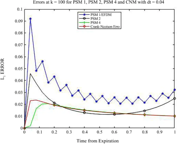
Figure 2. The absolute errors at S=100 for various PSM and CNM with dt=0.04.

[image:15.595.230.517.340.573.2]

DOI: 10.4236/jmf.2019.94031 631 Journal of Mathematical Finance Figure 2 is similar to Figure 1 but for a slightly larger time step, dt=0.04.

Here we can plainly see that the EFDM is far less accurate than all the other me-thods and begins to oscillate. This is due to the instability of the EFDM. The second order PSM (PSM 2) and fourth order (PSM 4) is as accurate as the CNM and everywhere more accurate than the EFDM. As the time step increases and EFDM becomes less stable, and loses accuracy. PSM 4 is as accurate as CNM and close to expiration sometimes more accurate. This implies that the PSM can be computed more quickly than both CNM and EFDM without losing accuracy. This is particularly important in a trading environment or any application where resources are constrained. As we extend our research to non-linear applications this property will become even more important.

A Note on Discontinuity

Cen and Le (2011) highlight many of the difficulties within numerical routines in dealing with the non-differentiability at the strike price. In Figure 2 we can see the oscillation aspects to some degree within the EFDM framework. The general symbolic PSM method cannot be used on a non-differentiable initial condition. Here we approximate the put payoff with an infinitely differentiable function which gives us advantages over Cen and Le [9]. This is a relatively common issue throughout continuous mathematics. Whenever an application contains a discrete boundary condition difficulties will arise by the very nature of differentiability. Consequently, numerical approaches like FDM and PSM will have to deal with this issue. As we illustrate below the PSM easily addresses this problem that can negatively impact the FDM approaches.

One reason that PSM does not work in a symbolic environment for BSMOPMPDE is that the payoff functions are not differentiable at the strike price, K since the payoff for a call is given by Q S

( )

=max

(

S−K, 0

)

and for a

put is given by Q S

( )

=max

(

K−S, 0

)

and to do PSM on a PDE the initial

condition must be infinitely differentiable. In the Appendix, we give the second degree polynomial approximation to V S

( )

,τ that Maple generated (The

fourth degree polynomial is too large to represent.) and the infinitely differenti-able Q we used to approximately the put payoff even at the discrete boundary condition.

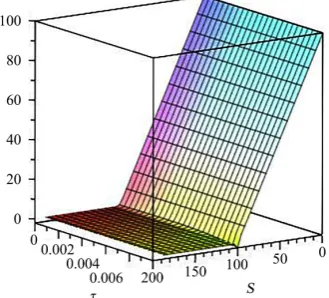
Figure 3 is a plot of the fourth PSM iterate given by Equation (6) for a call with r=0.03 , q=0.015 , σ =0.25 , K=100 over the time interval

0≤ ≤τ 0.01 (T−0.01≤ ≤t T) for 0≤ ≤S 200.

6. Conclusion

[image:17.595.291.456.77.226.2]

DOI: 10.4236/jmf.2019.94031 632 Journal of Mathematical Finance Figure 3. A Maple 3D Plot of a Put From a

Symbolic PSM Fourth Degree Polynomial.

speed increases) the advantages of PSM over EFDM becomes more apparent. Additionally, the PSM is everywhere as accurate as the CNM without the computational limitations. The PSM easily addresses discrete boundary condi-tions as well. Finally, due to the polynomial representation of PSM, analysts can far more accurately approximate values and hedging parameters for almost any set of inputs without being constrained by a finite difference grid. Future re-search will include more complicated nonlinear applications that will highlight the advantages over traditional FDM even more. These future applications offer fertile ground for research. Both FDM and CNM approaches struggle with non-linear applications. PSM offers a framework that doesn’t suffer the same limita-tions. PSM is an excellent alternative to the numerical finance literature.

Conflicts of Interest

The authors declare no conflicts of interest regarding the publication of this paper.

References

[1] Parker, G. and Sochacki, J. (1996) Implementing the Picard Iteration. Neural,

Pa-rallel, and Scientific Computation, 4, 97-112.

[2] Parker, G. and Sochacki, J. (2000) A Picard-McLaurin Theorem for Initial Value PDE’s. Abstract Analysis and Its Applications, 5, 47-63.

https://doi.org/10.1155/S1085337500000063

[3] Gofen, A.M. (2009) The Ordinary Differential Equations and Automatic Differen-tiation Unified. Complex Variables and Elliptic Equations, 54, 825-854.

https://doi.org/10.1080/17476930902998852

[4] Neidinger, R.D. (2010) Introduction to Automatic Differentiation and Matlab Ob-ject-Oriented Programming. SIAM Review, 52, 545-563.

https://doi.org/10.1137/080743627

DOI: 10.4236/jmf.2019.94031 633 Journal of Mathematical Finance [6] Stewart, R.D. and Bair, W. (2009) Spiking Neural Network Simulation: Numerical

Integration with the Parker-Sochacki Method. Journal of Computational

Neuros-cience, 27, 115-133.https://doi.org/10.1007/s10827-008-0131-5

[7] Rudmin, J.W. (1998) Application of the Parker-Sochacki Method to Celestial Me-chanics. Technical Report, James Madison University, Harrisonburg.

[8] Anwar, M. and Andallah, L. (2018) A Study on Numerical Solution of Black-Scholes Model. Journal of Mathematical Finance, 8, 372-381.

https://doi.org/10.4236/jmf.2018.82024

[9] Cen, Z. and Le, A. (2011) A Robust and Accurate Finite Difference Method for a Generalized Black-Scholes Equation. Journal of Computational and Applied

Ma-thematics, 235, 3728-3733.https://doi.org/10.1016/j.cam.2011.01.018

[10] Warne, P.G., Warne, D.A., Sochacki, J.S., Parker, G.E. and Carothers, D.C. (2006) Explicit A-Priori Error Bounds and Adaptive Error Control for Approximation of Nonlinear Initial Value Differential Systems. Computers & Mathematics with

Ap-plications, 52, 1695-1710.https://doi.org/10.1016/j.camwa.2005.12.004

[11] Carothers, D.C., Parker, G.E., Sochacki, J.S. and Warne, P.G. (2005) Some Proper-ties of Solutions to Polynomial Systems of Differential Equations. Electronic Journal

of Differential Equations, 40, 1-17.

[12] Carothers, D.C., Lucas, S.K., Parker, G.E., Rudmin, J.D., Sochacki, J.S., Thelwell, R.J., Tongen, A. and Warne, P.G. (2012) Connections between Power Series Me-thods and Automatic Differentiation. Recent Advancements in Algorithmic

Diffe-rentiation, 87, 175-186.https://doi.org/10.1007/978-3-642-30023-3_16

[13] Duffie, D. (2006) Finite Difference Methods in Financial Engineering: A Partial Differential Equation Approach. John Willy & Sons, Hoboken.

https://doi.org/10.1002/9781118673447

[14] Brennan, M. and Schwartz, E. (1978) Finite Difference Methods and Jump Processes Arising in the Pricing of Contingent Claims: A Synthesis. Journal of

Fi-nancial and Quantitative Analysis, 13, 461-474.https://doi.org/10.2307/2330152

[15] Company, R., Jodar, L. and Pintos, J.R. (2009) A Numerical Method for European Option Pricing with Transaction Costs Nonlinear Equation. Mathematical and

Computer Modelling, 50, 910-920.https://doi.org/10.1016/j.mcm.2009.05.019

[16] Forsyth, P. and Labahn, G. (2007) Numerical Methods for Controlled Hamil-ton-Jacobi-Bellman PDEs in Finance. Journal of Computational Finance, 11, 1-44.

https://doi.org/10.21314/JCF.2007.163

[17] Tangman, D., Gopaul, A. and Bhuruth, M. (2008) Numerical Pricing of Options Using Higher-Order Compact FD Schemes. Journal of Computational and Applied

Mathematics, 218, 270-280.https://doi.org/10.1016/j.cam.2007.01.035

[18] Buetow, G. and Sochacki, J. (1995) A Finite Difference Approach to the Pricing of Options Using Absorbing Boundary Conditions. Journal of Financial Engineering, 4, 263-280.

[19] Buetow, G. and Sochacki, J. (1998) A More Accurate Finite Difference Approach to the Pricing of Contingent Claims. Applied Mathematics and Computation, 91, 111-126.https://doi.org/10.1016/S0096-3003(97)10029-7

[20] Buetow, G. and Sochacki, J. (2000) The Tradeoffs between Alternative Finite Dif-ference Techniques Used to Price Derivative Securities. Applied Mathematics and

Computation, 115, 177-190.https://doi.org/10.1016/S0096-3003(99)00141-1

DOI: 10.4236/jmf.2019.94031 634 Journal of Mathematical Finance

https://doi.org/10.1137/060675186

[22] Leland, H. (1985) Option Pricing and Replication with Transactions Costs. The

Journal of Finance, 40, 1283-1301.

https://doi.org/10.1111/j.1540-6261.1985.tb02383.x

[23] Boyle, P. and Vorst, T. (1992) Option Replication in Discrete Time with Transac-tion Costs. The Journal of Finance, 47, 271-293.

https://doi.org/10.1111/j.1540-6261.1992.tb03986.x

[24] Hoggard, T., Whaley, A. and Wilmott, P. (1994) Hedging Option Portfolios in the Presence of Transaction Costs. Advances in Futures and Options Research, 7, 21-35. [25] Kratka, M. (1998) No Mystery behind the Smile. Risk, 9, 67-71.

[26] Jandacka, M. and Sevcovic, D. (2005) On the Risk-Adjusted Pricing-Methodology- Based Valuation of Vanilla Options and Explanation of the Volatility Smile. Journal

of Applied Mathematics, 3, 235-258.https://doi.org/10.1155/JAM.2005.235

[27] Barles, G. and Soner, H.M. (1998) Option Pricing with Transaction Costs and a Nonlinear Black-Scholes Equation. Finance and Stochastics, 2, 369-397.

https://doi.org/10.1007/s007800050046

[28] Kutik, P. and Mikula, K. (2011) Finite Volume Schemes for Solving Nonlinear Par-tial DifferenPar-tial Equations in Financial Mathematics. In: Finite Volumes for

Com-plex Applications VI and Perspectives, Springer, Berlin, 643-651.

https://doi.org/10.1007/978-3-642-20671-9_68

[29] Lesmana, D. and Wang, S. (2013) An Upwind Finite Difference Method for a Non-linear Black-Scholes Equation Governing European Option Valuation under Transaction Costs. Applied Mathematics and Computation, 219, 8811-8828.

https://doi.org/10.1016/j.amc.2012.12.077

[30] Frey, R. (2000) Market Illiquidity as a Source of Model Risk in Dynamic Hedging. In: Gibson, R., Ed., Model Risk, Risk Publications, London, 125-136.

[31] Frey, R. and Patie, P. (2002) Risk Management for Derivatives in Illiquid Markets: A Simulation Study. In: Sandmann, K. and Schnbucher, P., Eds., Advances in Finance

and Stochastics, Springer, Berlin, 137-159.

https://doi.org/10.1007/978-3-662-04790-3_8

[32] Frey, R. and Stremme, A. (1997) Market Volatility and Feedback Effects from Dy-namic Hedging. Mathematical Finance, 7, 351-374.

https://doi.org/10.1111/1467-9965.00036

[33] Liu, H. and Yong, J. (2005) Option Pricing with an Illiquid Underlying Asset Mar-ket. Journal of Economic Dynamics and Control, 29, 2125-2156.

https://doi.org/10.1016/j.jedc.2004.11.004

[34] Bakstein, D. and Howison, S. (2003) A Non-Arbitrage Liquidity Model with Ob-servable Parameters for Derivatives. Working Paper, Oxford Centre for Industrial and Applied Mathematics, Oxford, 1-52.

[35] Pruett, C.D., Rudmin, J.W. and Lacy, J.M. (2003) An Adaptive N-Body Algorithm of Optimal Order. Journal of Computational Physics, 187, 298-317.

https://doi.org/10.1016/S0021-9991(03)00101-3

[36] Nurminskii, E. and Buryi, A. (2011) Parker-Sochacki Method for Solving Systems of Ordinary Differential Equations Using Graphics Processors. Numerical Analysis

and Applications, 4, 223.https://doi.org/10.1134/S1995423911030049

[37] Pruett, C.D., Ingham, W.H. and Herman, R.D. (2011) Parallel Implementation of an Adaptive and Parameter-Free n-Body Integrator. Computer Physics

DOI: 10.4236/jmf.2019.94031 635 Journal of Mathematical Finance [38] Szynkiewicz, P. (2016) A Novel GPU-Enabled Simulator for Large Scale Spiking

Neural Networks. Journal Telecommunications and Information Technology, 2, 34-42.

[39] Yudanov, D., Shaaban, M., Melton, R. and Reznik, L. (2010) GPU-Based Simulation of Spiking Neural Networks with Real-Time Performance & High Accuracy. The

2010 International Joint Conference on Neural Networks (IJCNN), Barcelona,

18-23 July 2010, 1-8.https://doi.org/10.1109/IJCNN.2010.5596334

DOI: 10.4236/jmf.2019.94031 636 Journal of Mathematical Finance

Appendix.

In Figure 1 and Figure 2 we showed the errors for PSM 1, PSM 2 and PSM 4 and CNM for different time steps. Below we show the fourth degree polynomial generated by PSM 4 at S74 =74.

[ ]4

_{( )}

2 3

74

4

26 1.89 0.036675 0.000408374999996 0.000003218905924

v t t t t

t

= − + −

+

It is important to remember that PSM generates a polynomial for each Si and that from this polynomial we know that

[ ]3

_{( )}

2 3

74 26 1.89 0.036675 0.000408374999996

v t = − t+ t − t

is generated by PSM 3 and

[ ]2

_{( )}

2

74 26 1.89 0.036675

v t = − t+ t

Is generated by PSM 2.

In Figure 3 we generated the results for a put option using a smooth approx-imation to the put payoff using Maple. We actually plotted the fourth degree polynomial that Maple generated. The second degree polynomial Maple gene-rates for any V S

( )

, 0 =Q s r q

( )

, , and σ is

( )

( )

( )

(

)

( ) (

)

( )

( )

(

)

( )

( )

(

)

( )

4 2 2 4 2 3

2 2 2 2

2 3

2 3 2

2 3 2

3 2 2 3 2 2 2 d d

1 d d

2

4 d d 2

d d d

2

d d d

d d

1 d d

2 d 2 d

S Q S

S

S Q S S Q S

S S

r q Q S r q S Q S r Q S

S S S

S Q S

S

r q S S Q S r q Q S

S S

r

σ

σ σ σ

σ σ     _{     }      _{  + +}       _{     }           + −  + −  −  _      _             + _ − _  + + − _ _     + −

(

)

( )

( )

( )

(

)

( )

( )

( )

(

)

( )

( )

( )

2 2 2 2 2 2 2 2 2 2 2 d d d d d d d 2 d 2 d d d 2 d

q S Q S r Q S

S S

S Q S

r S

r q S Q S rQ S

S

S Q S

S

r q S Q S rQ S Q S

S σ τ σ τ   ₋      _                      _{+ − −}     _{ }    _{ } −                +_ + − _{ }− _ +    

We used Q S

( )

=ln 1 exp

(

+

(

S−100

)

)

− +S 100 to approximate the put

payoff for Figure 3. The maximum difference between this Q and the put payoff is ln2 and occurs at S=K=100. A future study would involve approximating