GPS Signal Short Term Propagation Characteristics Modeling in Urban Areas for Precise Navigation Applications

GPS Signal Short-Term Propagation Characteristics

Modeling in Urban Areas for Precise Navigation

Applications

G. Sateesh Kumar1, G. Sasi Bhushana Rao2,M. N. V. S. S. Kumar2

1_{Department of ECE, Aditya Institute of Technology and Management, Tekkali, India;} 2_{Department of ECE, Andhra University,}

Visakhapatnam, India.

Email: [email protected]

Received March 11th_{, 2013; revised April 10}th_{, 2013; accepted April 25}th_{, 2013}

Copyright © 2013 G. Sateesh Kumar et al. This is an open access article distributed under the Creative Commons Attribution Li- cense, which permits unrestricted use, distribution, and reproduction in any medium, provided the original work is properly cited.

ABSTRACT

GPS navigation signal includes vital information such as orbital parameters, clock error coefficients etc. This received signal which is extremely weak is affected by several errors during its propagation and is of the order of 10−16 _{W. The}

noise floor of this signal is 400 times higher than the transmitted signal. The situation becomes much worse particularly when the GPS receiver is located at urban areas where the multipath effect is predominant in the code and carrier phase measurements. GPS usage is not limited to the aircraft en-route navigation and missile guidance where the user receives the satellite signals from the open sky. At the present time, it has become an essential utility in the car navigation, mo- bile phones, surveying and aircraft landing application. The signal propagation characteristics particularly the short- term variations severely affect the quality, availability and continuity of the system. In this paper, short-term propaga- tion characteristics of GPS signal are modeled and analyzed. Short-term variations are mainly due to multipath reflec- tions and Doppler shift which degrades the quality of received signal particularly in urban environments. The variation of signal quality with respect to user velocity is observed using Rayleigh and Rician fading models.

Keywords: GPS; Navigation; Multipath; Rayleigh and Rician

1. Introduction

The Global Positioning System (GPS) is a satellite based modern navigation system that provides accurate three dimensional (3D) position, velocity and timing informa- tion up to 10−6 _{sec anywhere on or above the earth’s sur-}

face [1]. It is primarily designed as a land, marine, and aviation sector navigation system. Each GPS satellite transmits two spread spectrum pseudorandom noise (PRN) ranging codes along with 50 bps navigation data message at two frequencies L1 (1575.42 MHz) and L2 (1227.60 MHz) which are derived from highly stable on-board atomic clocks. The GPS receiver calculates its position by precisely timing the signals sent by satellites above the earth’s surface. The accuracy of the computed position depends on the received signal strength, which may degrade due to several reasons such as travelling long distances through vacuum, dense clouds, dust parti- cles, different layers of the earth’s atmosphere such as troposphere, ionosphere, protonosphere natural elements such as mountains, and even man-made flying objects

like airplanes etc. In addition, the random fluctuations in the received signals due to different fading phenomena also affect the signal quality, system availability and are ultimately a major cause of system outages.

Because the signal received over each path has a random amplitude and phase, the instantaneous value of the composite signal is found to vary randomly about a local mean [3]. In this paper, the short-term fluctuations in the GPS signal amplitude due to phase change is analyzed using Rayleigh and Rician fading models

2. Multipath

Multipath error is one of the predominant error sources in all GPS applications. Particularly the multipath error has to be precisely estimated in the Global Navigation Satel- lite Systems (GNSSs) as it is the major error source (2 - 4 m) that limits the GPS receiver’s performance [3]. When- ever, a signal is transmitted from a GPS satellite it fol- lows a “multiple” number of propagation “paths” on its way to receiving antenna. These multiple signal paths are due to the fact that the signal gets reflected back to the antenna off surrounding objects, including the earth’s surface.The GPS receiver tracks both the direct and re- flected signal components.

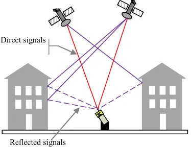
The radio wave transmitted from a satellite radiates in all directions, these radio waves including reflected waves that are reflected off due to various obstacles, dif- fracted waves, scattering waves, and the direct wave from the satellite to GPS receiver (see Figure 1). In this

case, since the path lengths of the direct, reflected, dif- fracted, and scattering waves are different, the time each takes to reach the GPS receiver will be different. In addi- tion the phase of the incoming wave varies because of reflections. As a result, the receiver receives a superpos- tion consisting of several waves having different phase and times of arrival.

The generic name of a radio wave in which the time of arrival is retarded in comparison with this direct wave is called a delayed wave. Then, the reception environment characterized by a superposition of delayed waves is called a multipath propagation environment. In a multi- path propagation environment, the received signal is sometimes intensified. This phenomenon is called multi-

Direct signals

[image:2.595.318.538.573.705.2]

Reflected signals

Figure 1. Principle of multipath signal.

path fading and the signal level of the received wave changes from moment to moment.

3. Fading

Fading is a common phenomenon in GPS caused by the superposition of two or more versions of the transmitted signals, which arrive at the receiver at slightly different times. The resultant received signal can vary widely in amplitude and phase, depending on various factors such as the relative propagation time of the waves and band- width of the transmitted signal. At the receiver, these multipath waves with randomly distributed amplitudes and phases combine to give a resultant signal that fluctu- ates in time and space. Therefore, a receiver at one loca- tion may have a signal that is much different from the signal at another location, only a short distance away, because of the change in the phase relationship among the incoming radio waves. This causes significant fluc- tuations in the signal amplitude. This phenomenon of random fluctuations in the received signal level is termed as fading. The short-term fluctuation in the signal ampli- tude caused by the local multipath is called Rayleigh fading, and is observed over distances of about half a wavelength. The most commonly known statistical rep- resentations of fading are: Rayleigh, Rician [4]. Received signal envelope in a typical multipath environment is shown in Figure 2.

4. Rayleigh Fading Model

A GPS receiver in a typical dense populated urban envi- ronment is usually surrounded by local scatterers so that the plane waves will arrive from many directions without a direct line of sight component. Two-dimensional iso- tropic scattering, where the arriving plane waves arrive in from all directions with equal probability is most com- monly used scattering model for the GPS system. For this type of scattering environment the received envelope is short-term distributed at any time, and is said to exhibit

Fade width Received signal

Envelope

Fade Fade level

= - R dB Average signal

level

λ/2

[image:2.595.83.270.575.719.2]

Distance from satellite

Rayleigh fading [5]. Such channels are modelled using Rayleigh fading model. Let us begin with the mechanism by which fading occurs. The delayed wave with incident angle n is given by Equation (1) corresponding to

Figure 1, when a continuous wave of single frequency,

c

f (Hz), is transmitted from the satellite. Delayed wave with incident angle, n

 



 

2π 

Re ej f tc



n n

r t  e t (1)

where, r t_n

 

delayed signal/phase difference;

c f 



carrier frequency;



Re indicates the real part of a complex number that gives the complex envelope of the incoming wave from the direction of the number, n;

j is a complex number.

The is calculated using the propagation path length of the incoming waves. n

 

e t

 

 

 

 

 

2π cos

e

n n

n

L vt

j

n n n n

e t R t x t jy t

   _  _       

   (2)

where R_n and_nare the envelope and phase of the nth

incoming wave.

 

n

x t and y t_n

 



n

e

are the in-phase and quadrature phase factors of t



, respectively.

v speed of GPS receiver;

  wavelength;

n

L  propagation path length2π 

 

L_n ;

n

  incident angle;

 wavelength;

Doppler shift v_ccos _n .

The incoming nth _{wave shifts the carrier frequency as}

 

cos

c n

v   z by the Doppler Effect (Hz). This is called the Doppler shift in GPS communication. This Doppler shift, which is described as _d, has a maximum value of v , when the incoming wave comes from the running direction of receiver in cosn1. Then, this

maximum is the largest Doppler shift. The delayed wave that comes from the rear of the receiver also has a fre- quency shift of d (Hz). It is shown by Equation (2),

since received wave received in GPS is the syn- thesis of the abovementioned incoming waves, when the incoming wave number is made to be N. Summation of N reflected signals

 

r t

 

 

 

 

 

 

















 

 

2π 1 1 Re e

Re cos 2π sin 2π

cos 2π sin 2π c

N N

j f t

n n

n n

c c

c c

r t

r t e t

x t jy t f t j f t x t f t y t f t

       _{  }        _   _  





(3)

where x t

 

and y t

 

are given by

 

 

1 N

n n

x t x







t and

 

 

1 N

n n

y t y







t (4)

 

x t and y t

 

are normalized random processes, having an average value of zero and dispersion of  , when N is large enough. The combination probability density p x

 

,y is given by,

 

2 2 2 2 2 1 , e 2π x y

p x y 



      

  ₍₅₎

where x x t y

 

, y t

 

.

In addition, it can be expressed as r t

 

using the am- plitude and phase of the received wave.

 

 

cos 2



πc

 



r t R t f t t (6)

 

R t and 

 

t are given by

 

2

R t _{ }R x _y2 _{and }

 

_{t   tan}1

 

_{y x .}

By using a transformation of variables, p x y

 

, can be converted into p R



,



. Short-term distribution of

, R is





2 2 2 2 , e 2π R R p R 



     

  ₍₇₎

By integrating p R



,



over θ from 0 to 2, we obtain the probability density function . Probability den- sity function of

 

p R

 

p R is

 

2 R   2 2 2e R p R 



     

 (8)

Moreover, we can obtain the probability density func- tion p

 

 by integrating p R



,



over R from 0 to ∞.

 

1

2π

p   (9)

From these equations, the envelope fluctuation follows a short-term distribution, and the phase fluctuation fol- lows a uniform distribution on the fading in the propaga- tion path. Next, let us try to find an expression for rayleigh fading. Here, the GPS receives the radio wave as shown in Figure 1, the arrival angle of the receiving in-

coming wave is uniformly distributed, and the wave number of the incoming waves is N. In this case, the complex fading fluctuation in an equivalent low pass sys- tem is

 

ejt

 

r t  x t  jy t

 

(10)

 





 





 





 





1 1 1 cos cos 1 sin cos 1 cos cos

1 _{sin cos}

N

d n n

n N

d n

n

d n n

d n n

where

n

 and n are uniformly distributed over 0 to 2π; d

 

N number of scatterers. Doppler shift frequency;

The Doppler frequency shift is calculated by

cos c d vf c  _{ } _ 

  (12)

where fc  carrier frequency;

v receiver velocity;

  elevation angle; c velocity of light.

Receiver velocity is positive when the receiver is moving towards the transmitter and negative when mov- ing away from the transmitter. The level crossing rate (LCR) and average fade duration (AFD) are given by the formula

2

2π e

Y d

L  w  (13)

2 e 1 2π Y d T w   

 (14)

where  fade level.

5. Rician Fading Model

It is a stochastic model for radio propagation anomaly caused by partial cancellation of radio signal by itself. If the environment is such that, in addition to scattering there is a strong dominant signal seen at the receiver caused by line of sight, the mean of the random process is no longer zero and varies around the power level of the dominant path. Such a situation may be better modelled as Rician fading. Rayleigh fading is a specialized model for Rician fading when there is no line of sight signal. In a microcellular environment, the transmitter antennas are often placed below the skyline of buildings and are sur- rounded by local scatterers, such that the plane waves will arrive at the base station with a larger AOA (Angle of Arrival) spread [6]. Furthermore, LOS path will some- times exist between the satellite and receiver, while at other times LOS path does not exist. Even in the absence of LOS propagation conditions, there often exist a domi- nant reflected or diffracted path between the satellite and receiver.

LOS or dominant reflected or diffracted path produces the specular component and the multitude of weaker secondary paths contributes to the scatter component of the received envelope. In this type of propagation envi- ronment, the received signal envelope still experiences fading. However, the presence of the specular component changes the received envelope distribution, and very of- ten a Rician distributed envelope is assumed. In this case the received envelope is said to exhibit Rician fading.

Such channels are modelled by Rician fading model. Rician distribution is used to model the GPS signal when a direct line of sight component exists between the ob- stacle and receiver in addition to the multipath compo- nents. It can be expressed as a phasor sum of a constant and a number of scattering point sources.

1

ej n ejj

j j

R r  C A 



  



(15)

where,

C constant coherent signal with clear LOS;

j

A  Amplitude of jth _{incoming wave;} j

  Initial phase shift of jth _{incoming wave.}

Rician probability density function is given by

 



2 2



0 2

2 e

r C _rC

I r

p r   r

  _    _  _{ }  _{  }  

  _{, 0}

  (16)

 

0, 0

p r  r (17) where  is the mean square value of the Rayleigh dis- tributed component of r and I0 is the modified Bessel

function of order zero. The phase distribution is no longer uniform like Rayleigh distribution. The phase distribution of Rician distribution is derived by Beck- mann as

 

1 2



2



 





e 1 πe 1

2π

C G

p  _   _G _e_{rf G (18)}

where G Ccos, 0  2π



   and

 

2

0 2 e d π G y

erf G 

_

 y

Clarke’s simulation model for simulating Rician fad- ing is given by the signal transfer function which is given by

 

 

 

 





1

1 _{cos cos}

c s

N

c d

n

Y t Y t jY t

Y t t

N   n n

 





 (19)

 





1

1 N _{sin cos}

s d n

n s

Y t t

N    n





 (20)

where N is the number of propagation paths;

d

 is the maximum Doppler frequency in radians;

n

 and n are the angle of arrival and initial phase

of the nth _{propagation path respectively.}

Both n and n are uniformly distributed over



π,π



for all n and they are mutually independent. The signal transfer function after including the direct LOS component is given by

 

 

 

 







cos cos 0 0



1

c s

c c d

Z t Z t jZ t

Z Y t K  t   K

 

 







sin cos 0 0



1

s s d

Z  Y t  K  t   K (22) sidering the carrier frequency to be 1575.42 MHz, num- ber of scatterers N8 and by changing the value of Doppler frequency shift

 

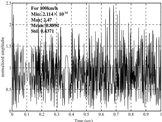
d . The value of N is

deter-mined from the environment. As the value of N increases, more accurate results are obtained. The response of Rayleigh fading is computed for different configuration. The response of Rayleigh fading of GPS satellite trans- mitted signal for a receiver moving velocity of 30 km/h is shown in Figure 3. From Figure 3, it is observed that

the normalized amplitude of GPS signal changes with respect to time when the receiver is moving with velocity of 30 km/h. The response of Rayleigh fading of GPS transmitted signal for receiver velocities of 60 km/h and 100 km/h are shown in Figures 4 and 5 respectively.

where K is the ratio of multipath to direct component,

0

 and 0 are angle of incidence and initial phase of

direct component respectively.

6. Results and Discussion

The main aim of the paper is to obtain the response of Rayleigh fading and Rician for a GPS transmitted signal for different velocities of receiver using sum of sinusoids method. The response of Rayleigh fading of GPS signal for different velocities of receiver is obtained using sum of sinusoids method. This response is obtained by con-

0 0.1 0.2 0.3 0.4 0.5 0.6 0.7 0.8 0.9 1

0 0.5 1 1.5 2 2.5

no

rm

al

iz

ed

am

pl

itub

e

Time (sec)

For 30km/hr Min: 2.11



10-16

[image:5.595.159.439.266.482.2]

Max: 2.479 Mean: 0.8995 Std: 0.4594

Figure 3. Rayleigh fading response of a typical GPS signal for receiver moving with a velocity of 30 km/h.

0 0.1 0.2 0.3 0.4 0.5 0.6 0.7 0.8 0.9 1

0 0.5 1 1.5 2 2.5

no

rm

al

ized

am

pl

itu

be

Time (sec)

For 60km/h Min: 2.114



10-16

[image:5.595.167.432.517.715.2]

Max: 2.431 Mean: 0.8902 Std: 0.4471

0 0.1 0.2 0.3 0.4 0.5 0.6 0.7 0.8 0.9 1 0

0.5 1 1.5 2 2.5

nor

m

al

iz

ed a

m

pl

itube

Time (sec)

For 100km/h Min: 2.114



10-16

[image:6.595.164.430.87.287.2]

Max: 2.47 Mean: 0.8891 Std: 0.4371

Figure 5. Rayleigh fading response of a typical GPS signal for receiver moving with a velocity of 100 km/h.

From Figures 3-5, it is concluded that the level cross-

ing rate of the response of receiver moving with velocity of 100 km/h is more than the level crossing rates of the responses of the receivers moving with velocities of 30 km/h and 60 km/h at a fade level of 1 and the average fade duration for a receiver moving velocity of 100 km/h is more in comparison with the average fade duration for receiver velocities of 30 km/h and 60 km/h at a fade level of 1. The values of minimum amplitude, maximum am-plitude, mean and Std’s (standard deviations) of GPS transmitted signal with receiver velocities of 30 km/h, 60 km/h and 100 km/h are also calculated. From Figures 3-5, it is observed that the mean and standard deviations

vary with change in the receiver velocity.

The Rician fading for a GPS signal for different ve- locities of receiver are obtained using sum of sinusoids method. The response is obtained by considering the car- rier frequency MHz, number of scatterers and by changing the value of Doppler frequency shift



1575.42 c

f 

8, 3,6 N K



d

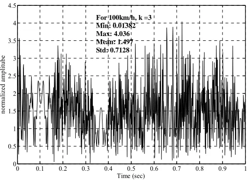
 . The value of N is determined from the environment. As in Rayleigh fading response, more accurate results are obtained for larger values of N. The response of Rician fading of GPS transmitted signal for a receiver moving velocity of 50 km/h and K3

and are shown in Figures 6 and 7. From these

Figures, it is observed that the normalized amplitude of GPS signal changes with respect to time when a receiver is moving with a certain velocity. From the Figures 6

and 7, it is also observed that as the value of K is in-

creased the normalized amplitude of response is reduced. The response of Rician fading of GPS transmitted signal for a receiver moving velocity of 100 km/h and

6 K

3 K

and are shown in Figures 8 and 9. From Figures 8 and 9, it is observed that the normalized amplitude of

GPS signal is changing with respect to time when a

re-ceiver is moving with velocity of 100 km/h. It is also observed that as the value of K is increased, the normal-ized amplitude of response is reduced.

6 K

From Figures 6-9, it is concluded that for a constant

value of K, the mean value of the response decreases with the increase in velocity of the user and for a con- stant velocity, as the value of K is increased the mean value is reduced. For constant K, the level crossing rate of the receiver moving with velocity of 100 km/h is more in compared with the level crossing rate of the receiver moving with velocity of 50 km/h at a fade level of 1. The average fade duration of a receiver with velocity 100 km/h is more in compared with the average fade duration of a receiver with velocity 50 km/h at a fade level of 1. The values of minimum amplitude, maximum amplitude, mean and standard deviations of GPS transmitted signal with receiver velocities of 50 km/h and 100 km/h are also calculated.

7. Conclusion

In this paper, modeling of short-term variations is pre- sented for the GPS transmitted signal. A short-term variation with Rayleigh fading model is analyzed for dif- ferent configurations (for example receiver moving with velocities of 30 km/h, 60 km/h and 100 km/h). From the analysis, it is concluded that the level crossing rate and the average fade duration of the receiver’s response due to Rayleigh fading is found higher at a fade level of 1 for a receiver moving with a velocity of 100 km/h in com- parison to the receiver moving with a velocity of 30 km/h. Short-term variations of the GPS signal using Rician fading model is also analyzed for different configurations (for example receiver with velocities 50 km/h and 100

m/h for

0 0.1 0.2 0.3 0.4 0.5 0.6 0.7 0.8 0.9 1

0 0.5 1 1.5 2 2.5 3 3.5 4

nor

m

al

ized am

pl

itube

Time (sec)

[image:7.595.171.425.86.278.2]

For 50km/h, k =3 Min: 0.03206 Max: 3.702 Mean: 1.563 Std: 0.7414

Figure 6. Rician fading response for a relative velocity of 50 km/h and K = 3 generated by sum of sinusoids method.

0 0.1 0.2 0.3 0.4 0.5 0.6 0.7 0.8 0.9 1

0 0.5 1 1.5 2 2.5 3

nor

m

al

ize

d a

m

pl

itub

e

Time (sec)

[image:7.595.171.424.310.504.2]

For 50km/h, k =6 Min: 0.04371 Max: 2.986 Mean: 1.345 Std: 0.6155

Figure 7. Rician fading response for a relative velocity of 50km/h and K=6 generated by sum of sinusoids method.

0 0.1 0.2 0.3 0.4 0.5 0.6 0.7 0.8 0.9 1

0 0.5 1 1.5 2 2.5 3 3.5 4 4.5

nor

m

al

iz

ed a

m

pl

itube

Time (sec) For 100km/h, k =3 Min: 0.01382 Max: 4.036 Mean: 1.497 Std: 0.7128

[image:7.595.172.425.533.718.2]

0 0.1 0.2 0.3 0.4 0.5 0.6 0.7 0.8 0.9 1 0

0.5 1 1.5 2 2.5 3 3.5

no

rm

al

ized

am

pl

itu

be

Time (sec)

[image:8.595.162.431.89.282.2]

For 100km/h, k =6 Min: 0.01531 Max: 3.295 Mean: 1.286 Std: 0.5955

Figure 9. Rician fading response for a relative velocity of 100 km/h and K = 6 generated by sum of sinusoids method.

that the level crossing rate and the average fade duration of the receiver’s response due to Rician fading is found higher at a fade level of 1 for a receiver moving with a velocity of 100 km/h in comparison to the receiver mov- ing with a velocity of 50 km/h.

REFERENCES

[1] G. S. Rao, “Global Navigation Satellite Systems with Es- sentials of Satellite communications,” McGraw Hill, New Delhi, 2010.

[2] B. Vucetic and J. Du, “Channel Modeling and Simulation in Satellite Mobile Communication Systems,” IEEE Jour-

nal on Selected Areas in Communications, Vol. 10, No. 8, 1992, pp. 1209-1218. doi:10.1109/49.166746

[3] P. Osborne and Y. J. Xie, “Propagation Characterization of LEO/MEO Satellite Systems at 900 - 2100 MHz,” Wil- liam University of Texas, Dallas, 1999.

[4] G. S. Rao, “Mobile Cellular Communication,” Pearson, 2012.