Munich Personal RePEc Archive
A Note on Nominal and Real
Devaluation in Laos
Kyophilavong, Phouphet and Shahbaz, Muhammad and
Salah Uddin, Gazi
National University of Laos, COMSATS Institute of Information
Technology, Lahore, Pakistan, Linköping University
9 July 2014
Online at
https://mpra.ub.uni-muenchen.de/57307/
1
A Note on Nominal and Real Devaluation in Laos
Phouphet Kyophilavong
Faculty of Economics and Business Management, National University of Laos,
POBOX7322, NUoL, Vientiane, Laos. Email: [email protected]
Muhammad Shahbaz Department of Management Sciences COMSATS Institute of Information Technology, Lahore, Pakistan. Email: [email protected]
Gazi Salah Uddin
Department of Management and Engineering Linköping University, SE-581 83 Linköping, Sweden
E-mail: [email protected]
Abstract
In this paper, we investigate whether or not nominal devaluation leads to real devaluation in
Laos by using the ARDL bounds testing and the Granger causality test in a VECM
framework. Our empirical evidence shows that nominal devaluation Granger causes real
devaluation in short run and long run. This finding implies that nominal devaluation leads to
real devaluation.
Keywords: Nominal devaluation, real devaluation, Laos
2
1. Introduction
The devaluation of the nominal exchange rate is a key policy to stimulate exports in many
LDCs. The nominal devaluation could improve the trade balance in two ways. First is by
making exports cheaper in terms of foreign currency that leads to an increase in the exports’
demand in international markets. Second is by making imports more expensive in terms of
domestic currency that leads to a decline in imports (Bahmani-Oskooee, and Kandil, 2007).
However, another cost of devaluation is an increase in the inflationary pressure that damages
the export sector and hence the whole economy. Therefore, investigating the relation between
real and nominal devaluation is crucial. The depreciation of the nominal effective exchange
rate could improve trade if the nominal devaluation leads to real devaluation only in short run,
and if it leads to depreciation of real effective exchange rate (Bahmani-Oskooee, 2001a;
Shahbaz, 2009).
However, the relation between nominal and real effective exchange rates is inconclusive in
the literature. Most studies find that the nominal devaluation leads to real devaluation in short
and medium runs (Vaubel, 1976; Connolly and Taylor, 1976, 1979; Bruno, 1978; Edwards,
1988, 1994). But some researchers find that nominal devaluation leads to real devaluation in
short and long runs; for instance, Bahmani-Oskooee and Miteza (2002) for 19 LDCs and
Bahmani-Oskooee and Kandil, (2007) for MENA. But, Holmes (2004) finds that nominal
devaluation does not lead to real devaluation in African countries. And, Bahmani-Oskooee
and Gelan, (2007) show that real devaluation results from nominal devaluation in medium
and long runs but in short run, the results is inconclusive. Bahmani-Oskooee and Harvey
(2007) investigate the relation between nominal and real devaluation by using data from
LDCs. They find that nominal devaluation leads to real devaluation. In single country studies,
Shahbaz, (2009) applies the ARDL bounds testing approach to establish a long-run relation
between both of the variables. The results indicate that nominal devaluation is positively
linked with real devaluation but that the causality is running from real to nominal devaluation
in Pakistan. In the Philippines, Wahid and Shahbaz, (2009) report that nominal devaluation
leads real devaluation in short run as well as in long run.
Laos has faced large chronic trade deficits since her independence in 1975. These trade
deficits accounted for 6.95 % of the GDP in 2011 (BOL, 2011). In addition, Laos also
experienced high inflation during the Asian financial crisis in 1997. Therefore, management
3
trade. Nominal and real effective exchange rates of industrial countries have been constructed
by the IMF since 1971. However, the IMF does not provide these rates for LDCs. The real
effective exchange rates for some LDCs were constructed by Bahmani-Oskooee (1995) and
Bahmani-Oskooee and Miteza (2002). However, Laos is not content with their studies.
Therefore, in this study, we construct nominal and real effective exchange rates’ indices.
However, to the best of our knowledge, there is no study investigating the relation between
these rates for Laos.1 This study is a pioneering effort to examine this relation for Laos by
using the ARDL bounds testing approach. This study contributes to the literature in three
ways. Firstly, it is a pioneering effort in investigating the relation between nominal and real
effective exchange rates in Laos. Secondly, the study uses the ARDL bounds testing
approach developed by Pesaran et al. (2001). Finally, we investigate the direction of causal
relation between nominal and real devaluations by applying the VECM Granger causality test.
The remainder of this paper is organized as follows. Section 2 describes the theoretical
framework and the empirical modeling. Section 3 contains the empirical results. Section 4
concludes.
2. Theoretical framework and empirical model
The empirical method follows Bahmani-Oskooee and Miteza (2002), Bahmani-Oskooee and
Kandil (2007), and Shahbaz (2009) who expanded the method. The empirical equation is
modeled as follows:
t t a a NEER
REER ln
ln 1 2 (1)
Where, REERt is real effective exchange rate, NEERt, is nominal effective exchange rate,
and
t is the error term. All of the series are converted into natural logarithms2. The studyconsists of quarterly data from 1993Q1 to 2010Q4. This time span is the longest period of
data that is available for Laos. The data on all of the variables comes from the International
1
Chansomphou and Ichihashi (2010) estimate the misalignment of the exchange rate in Laos.
Kyophilavong and Toyoda (2007) analyze the impact of the exchange rate on the Laos economy using a macroeconometric model.
2
4
Financial Statistics CD-ROM (2012). The calculation of REERt is based on
Bahmani-Oskooee and Miteza, (2002) and Bahmani-Bahmani-Oskooee and Kandil, (2007) and is shown below:
REERj=
∑
(
( ∗ / )
( ∗ / ) X 100) (3)
where REERj is an index of the real effective exchange rates in Laos, the Pj is the consumer
price index (CPI) in Laos, the Pi is CPI for trading partner i, EXRij is nominal bilateral
exchange rate between Laos and country i that is defined as the number of i’s currency per
unit of Laos’ currency (kip), then is the number of trading partners, the αij is the share of Laos’
import from trading partner i in the base period (1995), and the∑ = 1. The nominal
effective exchange rate (NEERj) is constructed the same way as the REERt:
NEERj=
∑
(
( )
( ) X 100) (4)
EXRij is defined as the number of units of i’s currency per unit of Laos’ currency (kip) that
indicates that the decrease in REERj and NEERj reflects the depreciation, and the increase
reflects the appreciation of Laos’ currency in real and nominal terms. This equation makes
possible the selection of Laos’ five main trading partners3.
We now apply Pesaran et al.’s (2001) ARDL bounds testing approach. A number of
advantages exist to this approach that can be compared to the Johansen cointegration
techniques (Johansen and Juselius, 1990).4 The ARDL bounds testing approach makes a
distinction between the dependent and explanatory variables. In order to implement the
bounds testing procedure, (1) is transformed to the unconditional error correction model
(UECM) below:
3
The main trading partners of Laos are Thailand, Vietnam, China, Korea, and Japan.
4
5 t t t p i i t i p i i t i t
u
NEER
REER
NEER
d
REER
c
c
REER
1 1 2 1 1 1 1 0ln
ln
ln
ln
ln
(5) t t t p i i t i p i i t i tu
NEER
REER
NEER
f
REER
e
d
NEER
2 1 2 1 1 1 1 0ln
ln
ln
ln
ln
(6)where denotes the first different operator, the c0and d0 are the drift components, p is the
maximum lag length, 5 and ut is the usual white noise residuals. The procedure of the ARDL
bounds testing approach has two steps. The first step is a F-test for the joint significance of
the lagged-level variables. The null hypothesis for the non existence of a long-run relation is
denoted by lnREERt/lnNEERt and H0:1= 2 =0 against Ha: 1≠ 2≠ 0. Pesaran et al.
(2001) generate lower and upper critical bounds for the F-test. The lower bound’s critical
values assume that all of the variables are I(0), while the upper bound’s critical values assume
that all of the variables are I(1). If the F-statistic exceeds the upper critical bound, then the
null hypothesis of no cointegration among the variables can be rejected. If the F-statistic falls
below the lower bound, then the null hypothesis of no long-run relation is accepted6. The next
step is the estimation of long-and-short run parameters by using the error correction model
(ECM). To ensure the convergence of the dynamics to long-run equilibrium, the sign of the
coefficient for the lagged error correction term (ECMt-1) must be negative and statistically
significant. Further, the diagnostic tests comprise the testing for the serial correlation,
functional form, normality, and the heteroscedasticity (Pesaran and Pesaran, 2009).
Once the variables are cointegrated for the long-run relation, then long- as well as short-run
causality can be investigated (Tiwari and Shahbaz, 2013; Shahbaz and Rahman, 2012). The
existence of a long-run relation between nominal and real effective exchange rates requires us
to detect which direction the causality takes between the variables by applying the VECM
5Pesaran et al. (2001) cautions that it is important to balance choosing the lag length. 6
6
(vector error correction method) Granger causality framework. The vector error correction
method (VECM) is as follows:
t t t t t i i i i p i t t ECM NEER REER b b a a L NEER REER L 2 1 1 1 1 2 1 22 21 12 11 1 2 1 ] [ ln ln ) 1 ( ln ln ) 1 ( (7)where the difference operator is (1L)and the ECMt1 is generated from long-run relation.
The long-run causality is indicated by the significance of the coefficient for the ECMt1 by
using the t-test statistic. The F statistic for the first differenced lagged independent variables
is used to test the direction of short-run causality between the variables.
3. Empirical results
The critical bounds are based on the assumption that the variables are I(0) or I(1) (Pesaran et
al. 2001; Narayan, 2005). Therefore, before conducting the bounds test for cointegration, we
apply a unit root test to make sure that our variables are not ordered at I(2), otherwise the
F-test could be spurious if the variables are stationary at the second difference (Ouattara, 2004).
We apply the augmented Dickey-Fuller (ADF) (Dickey and Fuller, 1979, 1981) and PP test
(Phillips and Perron, 1988). The results of the unit root test show that lnNEERt and
t
REER
ln are stationary at their different forms with the intercept and the trend (Table-1). This stationarity implies that our variables are ordered at I(1).
Table-1: Unit Root Test
Variable
ADF PP
Level Difference Level Difference
Intercept With
Trend Intercept
With
Trend Intercept
With
Trend Intercept
With Trend t REER ln -1.1776 [0.6810] -2.0896 [0.5439] -8.3024* [0.0000] -4.9091* [0.0008] -1.3713 [0.5927] -1.8474 [0.6728] -11.1791* [0.0001] -11.2713* [0.0000] t NEER ln -1.5418 [0.5073] -1.3037 [0.8796] -2.1016 [0.2447] -2.3186 [0.4189] -1.0455 [0.7337] -1.0207 [0.9351] -5.2858* [0.0000] -5.3293* [0.0002]
7
We select the optimal lag length based on the AIC. The result indicates that two is the
optimal lag order7. In order to account for the fact that we have a relatively small sample size,
we produce new critical values for the F-test that are computed with stochastic simulations
that use 20,000 replications. Table-2 reports the computed F-statistics that test for the
long-run relation between the variables.
Table-2: The Results of the ARDL Cointegration Test
Dependent Variable
t
REER
ln
F-statistics 5.692**
Critical values 5 per cent level 10 per cent level
Lower bounds 5.041 4.092
Upper bounds 5.867 4.839
Adi R-square 0.273
F-Statistics 2.610
Durbin Watson Test 1.892
Note: ** shows the significance at 5% level.
When lnREERt is dependent variable, then our calculated F-statistic is
) ln
/
(lnREERt NEERt
F = 5.692 and is greater than upper critical bound at 10% level of
significance. In addition, F-statistic suggests that there is cointegration between lnREERt
and lnNEERt in Laos. The long and short runs are shown in Table 3. In long run, nominal effective exchange rate is not statistically significant enough to determine lnREERt because
t
REER
ln equation has relatively weak cointegration. The F-value exceeds upper critical bound at 10% significance level but falls between lower and upper bounds at 5% significance
level. This result is consistent with Bahmani-Oskooee and Gelan (2006) for some African
countries, Shahbaz, (2009) for Pakistan, and Bahmani-Oskooee and Kandil (2007) for some
Middle Eastern and North African countries. In short run, the empirical evidence shows that
t
NEER
ln has a positive and significant impact on lnREERt. This impact implies that
7
8
devaluation of lnNEERt leads lnNEERt in short run. However, the estimate of ECMt-1 is
statistically significant with a negative sign at 5% level of significance. This finding shows
the speed of adjustment from short run to long run. We find that the deviations in short run to
long run are corrected by 20.30% in each quarter that shows the low speed of adjustment in
t
REER
ln model. The diagnostic tests are also applied for the adequacy of specification of model. The diagnostic tests suggest that the estimates are free from serial correlation and
misspecification of short-run model, and heteroskedasticity (Table-4).
Table-3: Long-run and Short-run Analysis
Dependent Variable = lnREERt
Long-run Results
Variable Coefficient T-Statistic
Constant 2.037* 107.388
t
NEER
ln -0.012 -1.042
Short-run Results
Variable Coefficient T-Statistic
Constant 0.006* 3.429
t
NEER
ln
0.477* 9.326
1
t
ECM -0.203* -5.620
Note: * denotes the significant at 1per
cent level respectively.
Table-4: Diagnostic Tests for lnREERtas Dependent Variables
F-version LM-version
Statistics P- Value Statistics P- Value
A: Serial Correlation F(4, 79)=1.798 0.137 2 (4)=7.178 0.127
B: Functional Form F(1, 82)= 1.510 0.223 2 (1)=1.555 0.212
C: Normality N/A 2 (2)=69.393 0.000
9
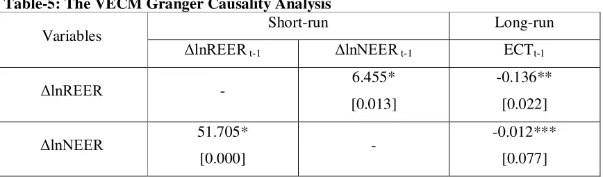
Table-5: The VECM Granger Causality Analysis
Variables Short-run Long-run
ΔlnREER t-1 ΔlnNEER t-1 ECTt-1
ΔlnREER - 6.455*
[0.013]
-0.136**
[0.022]
ΔlnNEER 51.705*
[0.000] -
-0.012***
[0.077]
Note: *, ** and *** denote the significant at 1, 5 and 10%levels respectively
Table 5 reports the results of Granger causality. The Table-5 shows that the estimates of
1
t
ECM are statistically significant with negative signs at 1% level. The statistical
significance of ECMt1 indicates the shock exposed by the system converging to long-run
equilibrium path. In long run, we find that the causality direction is from lnNEERt to
t
REER
ln and same is true from the opposite side. The feedback effect exists between
t
REER
ln and lnREERt in short run. This finding suggests that devaluation of nominal effective exchange rate leads to devaluation of real effective exchange rate in long run as well
as in short run.
4. Conclusion and Recommendations
The relation between nominal and real effective exchange rates is crucial for improving the
trade balance. Therefore, we investigate this relation in Laos. The empirical evidence shows
that the causality runs from nominal devaluation to real devaluation and vice versa in short
run and long run. This evidence implies that devaluation of nominal exchange rate leads to
devaluation of real exchange rate in Laos. This direction is crucial for policy makers in order
to better formulate the exchange-rate policy that improves the trade balance. Since Laos has
suffered from a trade balance and the monetary authority has adapted the manage-floating
exchange-rate regime (Kyophilavong, 2010), devaluation of nominal exchange rate might be
considered in order to improve the trade balance in short-and-long runs. But as Laos imports
most of its materials, the side effect from devaluation, namely inflationary effects, should
10
Acknowledgement
The authors are grateful to the anonymous referees of the journal for their extremely useful
suggestions to improve the quality of the paper. Usual disclaimers apply.
References
Bahmani-Oskooee, M., 1995. Nominal and real effective exchange rates for 22 LDCs: 1971:1-1990: 4. Applied Economics 27, 103-111.
Bahmani-Oskooee, M., 2001a. Nominal and real effective exchange rates of Middle Eastern countries and their trade performance. Applied Economics 33, 103-111.
Bahmani-Oskooee, M., 2001b. How stable in M2 money demand function in Japan?. Japan and the World Economy 13, 455-461.
Bahmani-Oskooee, M.,Gelan, A., 2006. Real and nominal effective exchange rates for African countries. Applied Economics 39(8), 961-979.
Bahmani-Oskooee, M., Kandil, M., 2007. Real and nominal effective exchange rates in MENA countries: 1970-2004. Applied Econometrics 39, 2489-2501.
Bahmani-Oskooee, M., Miteza, I., 2002. Do nominal devaluations lead to real devaluation in LDCs?. Economics Letter 74, 385-391.
Bahmani-Oskooee, M., Gelan, A., 2006. On the relationship between nominal devaluation and real devaluation: Evidence from African Countries. Journal of African Economies 16(2), 177-197.
Bahmani-Oskooee, M., Harvey, H., 2007. Real and nominal effective exchange rate for LDCs: 1971-2004. The International Trade Journal 21(4), 385-416
Bentzen, I., Engsted, T., 2001. A revival of the autoregressive distributed lag model in estimating energy demand relationship. Energy 26, 45-55.
BoL., 2011. Annual Report 2010-2012, the Bank of Lao PRD. Vientiane: The Bank of Lao PDR.
Bruno, M., 1978. Exchange rates, import costs, and wage-price dynamics. Journal of Political Economy 86, 379-403.
Chansomphou, V., Ichibashi, M., 2010. Foreign currency inflow, real exchange rate
misalignment and export performance of Lao PDR, 12th International Convention of the East Asian Economic Association, 2-3 October, Seoul.
Connolly, M., Taylor, D., 1979. Adjustment to devaluation with money and non-traded goods. Journal of International Economics 6, 289-298.
11
Dickey, D., Fuller, W.A., 1979. Distribution of the Estimates for Autoregressive Time Series with a Unit Root. Journal of the American Statistical Association 74, 427-431.
Dickey, D., Fuller, W.A., 1981. Likelihood Ratio Statistics for Autoregressive Time Series with a Unit Root. Econometrica 49, 1057-72.
Edwards, S., 1988. Exchange rate misalaignment in developing countries, World Bank Occasional Papers, No. 2, New Series, Baltimore: The Johns Hopkins University Presss.
Edwards, S., 1994. Exchange rate misalignment in developing countries. In: Barth, R., Wong, C. (Eds.). Approaches to exchange rate policy: Choices for Developing and Transition
Economies, Washington, DC: International Monetary Fund.
Ghatak, S., Siddiki, J., 2001. The use of ARDL approach in estimating virtual exchange rate in India. Journal of Applied Statistics 28, 573-583.
Holmes, M. J., 2004. Can African countries achieve long-run real exchange rate depreciation through nominal exchange rate depreciation?. South African Journal of Economics 72(2), 305-323.
Johansen, S., Juselius, K., 1990. Maximum likelihood estimation and inference on
cointegration with application to the demand for money. Oxford Bulletin of Economics and Statistics 52, 169-210.
Kremers, J. J., Ericson, N. R., Dolado, J. J., 1992. The power of cointegration tests. Oxford Bulletin of Economics and Statistics 54, 325-347.
Kyophilavong, P., Toyoda, T., 2007. Unfavorable Truth of Currency Integration – The Case of Laos. Journal of Economic Sciences 11(1), 1-17.
Kyophilavong, P., 2010. Lao People’s Democratic Republic: Dealing with Multi Currencies in: Capannelli, G., Menon, J. (Eds.). Dealing with Multiple Currencies in Transitional Economies, Manila: Asian Development Bank, 72-100.
Layson, S., 1983. Homicide and deterrence: Another view of the Canadian time-series evidence. The Canadian Journal of Economics 16(1), 52-73.
Narayan, P. K., 2005. New evidence on purchasing power parity from 18 OECD countries. Applied Economics 37, 1063–1071.
Ouattara, B., 2004. Modelling the long run determinants of private investment in Senegal, The School of Economics Discussion Paper Series 0413, Economics, The University of Manchester.
Pesaran, M. H., Shin, Y., Smith, R.J., 2001.Bounds testing approaches to the analysis of level relationships. Journal of Applied Economics 16, 289-326.
12
Phillips, P. C., Perron, P., 1988. Testing for a Unit Root in Time Series Regression. Biometrika 75(2), 335-46.
Shahbaz, M., Jalil, A., Islam, F., 2012. Real Exchange Rate Changes and the Trade Balance: The Evidence from Pakistan. The International Trade Journal 26(2), 139-153.
Shahbaz, M., 2009. On nominal and real devaluations relation: an econometric evidence for Pakistan. International Journal of Applied Econometrics and Quantitative Studies 9, 85-108.
Shahbaz, M., 2010. Income inequality-economic growth and non-linearity: a case of Pakistan. International Journal of Social Economics 37, 613-636.
Vaubel, R., 1976. Real exchange rate changes in the European community: The empirical evidence and its implications for European currency unification. WeltwirtschaftlichesArchiv 112, 429-470.
Wahid, A. N. M., Shahbaz, M., 2009. Does nominal devaluation precede real devaluation? The Case of the Philippines. Transition Studies Review 16(1), 47-61.
Tiwari, A. K., and Shahbaz, M (2013).Modelling the Relationship between Whole Sale Price and Consumer Price Indices: Cointegration and Causality Analysis for India ,Global Business Review,14, 397-411.