Linear Prolate Functions for Signal Extrapolation with Time Shift

(1)

http://www.scirp.org/journal/am ISSN Online: 2152-7393

ISSN Print: 2152-7385

Linear Prolate Functions for Signal

Extrapolation with Time Shift

Daniela Valente, Michael Cada, Jacek Ilow

Department of Electrical and Computer Engineering, Dalhousie University, Halifax, Canada

Abstract

We propose a low complexity iterative algorithm for band limited signal extrapolation. The extrapolation method is based on the decomposition of fi-nite segments of the signal via truncated series of real-valued linear prolate functions. Our theoretical derivation shows that given a truncated series (up to a selectable value) of prolate functions, it is possible to extrapolate the band limited function elsewhere if each extrapolated portion of the function is sub-ject only to moderate truncation errors that we quantify in this paper. The ef-fects of different sources of errors have been analyzed via extensive simula-tions. We have investigated a property of the signal decomposition formula based on linear prolate functions whereby the integration interval does not need to be symmetric with respect to the origin while time-shifted prolate functions are used in the series.

Keywords

Real-Valued Band Limited Eigenvectors, Signal Decomposition, Signal Extrapolation

1. Introduction

In the early 60’s David Slepian and his colleagues discovered the bandlimited function that is maximally concentrated, in the mean-square sense, within a given time interval; this function is the prolate spheroidal wave function (PSWF) of zero-order.

The linear prolate functions (LPFs) are the one-dimensional version of the prolate spheroidal functions and they form sets of bandlimited functions which are orthogonal and complete over a finite interval. Moreover, unlike other functions, they are also complete and orthogonal over the infinite interval. An additional property is that the finite Fourier transform (FT) of a linear prolate function is proportional to the same prolate function. Although there are other How to cite this paper: Valente, D., Cada,

M. and Ilow, J. (2017) Linear Prolate Func-tions for Signal Extrapolation with Time Shift. Applied Mathematics, 8, 417-427.

https://doi.org/10.4236/am.2017.84034

Received: February 10, 2017 Accepted: April 10, 2017 Published: April 13, 2017

http://creativecommons.org/licenses/by/4.0/

(2)

functions which are their own infinite Fourier transform, only the prolate functions enjoy the property for the finite transform: this property uniquely defines the prolate functions [1]. Associated with each function, there is an eigenvalue λn

( )

c and a free parameter c which is a useful descriptor of sys-

tem performance [2]. Some of the mentioned mathematical properties make the prolate functions easily applicable to optics [3]. In particular, we are interested in the problem of determining a bandlimited function from the knowledge of a finite segment of the function, since it is relevant in many practical situations from application to filters in communication systems [4] to optical systems when, for example, due to intrinsic instrumental limits, only limited observation data are available.

Specifically, in the research area of bandlimited signal extrapolation, there have been contributions with iterative and non-iterative algorithms for extrapolation of signals in the LCT (linear canonical transform) domain that is a generalization of the Fourier transform. The challenges of convergence of algorithms based on the Gerchberg-Papoulis (GP) algorithm [5] and an application to high frequencies have been extensively investigated [6]. However, approaches based on the use of the prolate spheroidal wave functions [7] need to provide efficient ways to compute the prolate functions.

In this paper, we benefit from a proprietary algorithm developed theoretically and implemented numerically by Cada [8], for accurate generation of linear prolate functions with desired high precision to use LPFs for signal extrapolation. In what follows, we introduces the basics of signal expansion using the linear prolate functions in Section 2; Section 3 presents our approach to signal extrapolation based on LPFs. In Section 4 and Section 5 simulation results, error analysis and numerical examples are presented and discussed. Finally conclu- sions are drawn in Section 6.

2. Signal Expansion

As sets of bandlimited functions, orthogonal on the finite interval and orthonormal on the infinite interval, the linear prolate functions ψ_n

( )

c t, can

be successfully used for the expansion of a generally complex, bandlimited function f t

( )

:

( )

0

, n n n

f t a

ψ

c t

∞

=

∑

₍₁₎

the representation is valid for all t, the bandwidth parameter is c= Ωt₀ ₀ where Ω0 represents the finite bandwidth or a cutoff frequency, and t0 is the time interval. The function f t

( )

is supposed to be Ω₀-bandlimited. Adopting

the criterion of a minimized mean-square error, the expansion coefficients an

in (1) are given by:

( ) ( )

, d

n n

a ∞ f t ψ c t t

−∞

=

_∫

(2)

There is an alternative way to derive the coefficients an using only the values

(3)

eigenvalues λn

( )

c . After multiplying (1) by ψm

( )

c t, , integrating as reported

in [1] and from the orthogonality properties of the LPFs which are valid on both the finite and infinite interval, one can obtain:

( )

0

( ) ( )

0

1

, d

t

n n _t n

a = _λ c _−

∫

₋ f t ψ c t t (3)

The latest expression for { }an together with (1) states that when the

bandlimited function f t

( )

is known over a finite interval of extend 2t₀ then

( )

f t is theoretically known everywhere if one can accurately calculate the

coefficients an for n → ∞, the functions ψn

( )

c t, and the eigenvalues λn

( )

c .

( )

n c

λ can be regarded as the index of energy concentration of each function

n

ψ _in

[

−t t₀,₀

]

. Therefore:

( )

0

( ) ( )

0

1

0

, , d

N _t

n n _t n

n

f t

λ

c −

ψ

c t ₋ f t

ψ

c t t

=

′ ′ ′  

 

∑

∫

 (4)

Accurate computing of ψn, λn and an for n>2c π (where Ncrit =2c π

is known as the critical value) turns the orthogonal expansion expression presented in (1) into a signal extrapolation problem. Indeed, for any LPFs set with a fixed c, the energy concentration of the functions within

[

−t t0,0

]

decreases as the order n increases and for n=Ncrit, the signal’s maximum

concentration reaches the boundary of the observation interval. Hence the summation of

{

λn

( )

c

}

is mostly determined by the first Ncrit terms whose

individual value is very close to 1, and the series n0λn

( )

c

∞ =

∑

converges to a

finite value

(

2c π

)

, as extensively analyzed in [9]. Accurate estimation of the

overlap integral 0

( ) ( )

0

, d

t

n t f t ψ c t t

−

∫

for high orders of n becomes then a

challenging problem of high-precision numerical integration with an absolute necessity of having ψ_n

( )

c t, with a high precision as well [8].

3. Signal Extrapolation

Our main objective in signal extrapolation using linear prolate functions aims to take advantage of a generalized expression stated in [3], never exploited so far, for the coefficients in (3) which enables the finite interval 2t0 to not be nece- ssarily symmetric with respect to the origin. Hence, for a general interval

0 0

T− ≤ ≤ +t t T t , relation (4) becomes:

( )

(

)

0

( ) (

)

0

1

0

, , d

N _{T t}

n n _{T t} n

n

f t

λ

c −

ψ

c t T ₋+ f t

ψ

c t T t

= ′ ′ ′ − −    

∑

∫

 (5)

Substituting y= −t′ T , the following expression for f t

( )

is obtained:

( )

(

)

0

(

) ( )

0

1

0

, , d

N _t

n n _t n

n

f t

λ

c −

ψ

c t T ₋ f y T

ψ

c y y

=

− +

   

∑

∫

 (6)

with

( )

_{( )}

0

(

) ( )

0 1

, d

t

n _t n

n

a T f y T c y y

c ψ

λ −

=

_∫

+ (7)

(4)

{ }

an , one can use (6) to perform the signal extrapolation on f t

( )

beyond the

observation interval

[

−t t0, 0

]

using an iterative approach.

Specifically, we start from the assumption that the function f t

( )

is perfectly

known in the interval

[

−t t0, 0

]

. We use (6) with T =0 to extrapolate the signal by an interval ( )0

t

∆ _{using already proposed algorithms to obtain accurate}

calculations of a_n

( )

0 till N =N( )0 >2c π. Instead of pursuing the more challenging computing for N2c π, Formula (6) is re-applied for T = ∆t( )0 to extrapolate the signal by an additional interval ( )T

t

∆ via accurate calculations of a Tn

( )

to

( )T ₂ _π

N > c . The procedure is then repeated for the i-th

iteration and up to the number of iterations that has been set. Specifically, at each iteration i, we form the function which becomes the input for iteration

1 i+ :

( )

(

)

( )

(

)

1

1 0 0

0 0

( )

, 1

i i i i t

i

f t f t f t f t p t

f t t i t t t i t

f t t i t t t i t

− ∆

−

 

= +_ − _

− + ∆ ≤ ≤ + − ∆ 

= 

+ − ∆ < ≤ + ∆ 

 



(8)

with f ti

( )

being defined in (6). For the sake of simplicity ∆t is chosen to be

the same at every iteration. Also,

( )

1, 0 0

(

1

)

0, otherwise

t

t i t t t i t

p_∆ t =  − + ∆ ≤ ≤ + − ∆



4. Numerical Results

A LPFs set with bandwidth parameter c=20π and t0=1 is used as the orthogonal basis for the proposed extrapolation method. The functions are discretized in time at a sampling rate of 0.001 for numerical implementation and each discrete sample has a high numerical precision greater than 100 digits. The software Mathematica characterized by high precision computing has been used for the simulations. Extrapolation is carried out on the Ω0-bandlimited test function shown in Figure 1.

( )

cos 2π π cos 2π cos 3π

11 7 2

t t

f t = _ t− _{ }_+ _ _− _ _

     

 

4.1. Perfect Knowledge of

f t

( )

in the Integration Interval

In order to test the proposed approach for signal extrapolation as described in Section 3, we consider the ideal case first. This assumption means that at each iteration of the extrapolation, the function f t T

(

+

)

in the integral in (6) is

known in Mathematica user-defined precision. Figure 2 shows reconstruction/ extrapolation after the first iteration when the time shift is T =0, the truncation

value is N =97 and the Mathematica built-in interpolation and integration

(5)

[image:5.595.224.525.76.501.2]

Figure 1. f t

( )

in the interval

[

−1,1

]

.

[image:5.595.226.523.77.275.2]

Figure 2. Extrapolated f t

( )

, no time shift.

[image:5.595.227.527.523.715.2]

(6)

tional interval which is up to the 60% of half of the time range where the

function is known. The presence of the truncation error is discussed in Section 5.

4.2. Estimate of

f t

( )

in the Integration Interval

We consider a more realistic case when the function f t

(

+T

)

in the integral in

(6) is known in Mathematica user-defined precision only for T =0. Figure 4(b)

shows signal reconstruction/extrapolation after 16 iterations with a total time shift T = − ⋅ ∆ =

(

i 1

)

t 0.3 and N =97.

Figure 4(c) shows results after 36 iterations with a total time shift T =0.7

and N=97. Each progressive shift is equal to ∆ =t 0.02. At every iteration 1

i+ , we use the function f ti

( )

as the new input to (6) to make the integral

calculation successful. The piecewise polynomial interpolation method presented in [10] has been applied for the accurate computing of the overlap integral and the LPFs set with bandwidth parameter c=20π has been used. Indeed, in

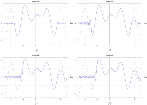
terms of the normalized mean-squared error (NMSE), the method in [10] performs superiorly when compared to the iterative approach proposed in [6] and the generalized PSWFs (prolate spheroidal wave functions) expansion method proposed in [7]. Specifically, for comparison purposes, Figure 4(a) is

(a) (b)

(c) (d)

Figure 4. Extrapolation outputs. (a) f t

( )

known in

[

−1,1

]

, i=1; (b) f t

( )

known in

[

−0.7,1.3

]

, i=16; (c) f t

( )

known in

[image:6.595.60.537.358.699.2]

(7)

obtained by setting i=1 and hence T =0, and reproduces results presented in

[10].

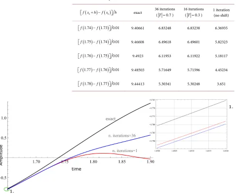
In Figure 5, details are shown for the extrapolation of the portion of the function in the time interval

[

1.65,1.9

]

. Despite the effect of accumulated

errors, it verifies that given the same truncation value N, the shift-approach

(i=36) outperforms the reference approach (i=1) when the extrapolation

capability of the reference approach vanishes.

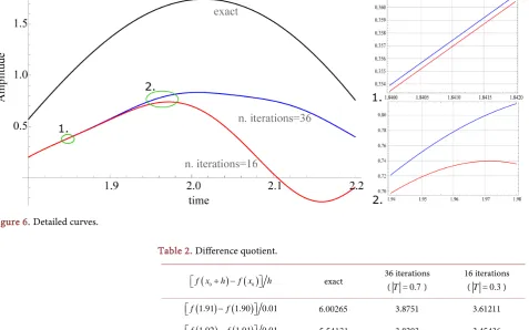
The difference quotients in Table 1 calculated between time instant 1.73 and time instant 1.78 are indices of the curves slope and show that the shift-approach follows better the slope of the exact function. In Figure 6, extrapolation details are shown for the portion of the function in the time interval

[

1.85, 2.2

]

.

Despite the effect of accumulated errors, the shift-approach for i=36 outper-

forms the shift-approach for i=16. The difference quotients in Table 2 calcu-

lated between time instants 1.90 and 2.00 show that the shift-approach for

36

[image:7.595.63.542.320.713.2]

i= follows better the slope of the exact function.

Table 1. Difference quotient.

(

0

)

( )

0

f x +h −f x h

 

  exact 36 iterations ₍_T ₌_0.7₎ 16 iterations ₍_T ₌_0.3₎ 1 iteration _{(no shift)}

(1.74) (1.73) 0.01

f −f

 

  9.40661 6.83248 6.83238 6.36935

(

1.75

)

(

1.74

)

0.01

f −f

 

  9.46608 6.49618 6.49601 5.82323

(1.76) (1.75) 0.01

f −f

 

  9.4923 6.11953 6.11922 5.18117

(1.77) (1.76) 0.01

f −f

 

  9.48503 5.71649 5.71596 4.45234

(

1.78

)

(

1.77

)

0.01

f −f

 

  9.44413 5.30341 5.30248 3.651

(8)

[image:8.595.66.537.75.752.2]

Figure 6. Detailed curves.

Table 2. Difference quotient.

(

0

)

( )

0

f x +h −f x h

 

  exact 36 iterations ₍_T _{= 0.7}₎ 16 iterations ₍_T ₌_0.3₎

(1.91) (1.90) 0.01

f −f

 

  6.00265 3.8751 3.61211

(1.92) (1.91) 0.01

f −f

 

  5.54131 3.8203 3.45436

(1.93) (1.92) 0.01

f −f

 

  5.05783 3.67135 3.16975

(1.94) (1.93) 0.01

f −f

 

  4.55379 3.41957 2.74234

(2.00) (1.99) 0.01

f −f

 

  1.19338 0.532228 −2.40967

5. Error Analysis

The proposed method is subject to an inherent series truncation error. Its mean squared error expression is the following, after an extrapolation interval Te:

( )

0 0 0

2 2 2

d d d

e e

t T t t T

T _t N _t N _t N

E =

∫

₋+ + f t − f t t=

∫

₋+ f t −f t t+

∫

₊+ + f t −f t t(9)

( )

0

( )

0 2 2 1 d e t T

n n _t N

n N

a

λ

c f t f t t

∞ _{+ +}

+ = +

=

∑

+

_∫

− (10)

The first term in the summation in (9) represents the error in the fit of fN

( )

t

(defined in (6)) to f t

( )

within the interval

[

−t t₀,₀

]

. Specifically, as reported

in [1], the calculation of 0

( )

0

(

( )

)

0 0

2 2

1

d , d

t t

N n N n n

t f t f t t t aψ c t t

+ + ∞

= +

− − = −

∑

∫

into

the sum form in (10) follows from the fact that ψ_n

( )

c t, are orthogonal on the

interval

[

−t t0, 0

]

. The term

( )

0 0 2 d e t T N

t f t f t t

+ +

+ −

∫

is the truncation error in

the extrapolation interval and then depends on the quantity Te. It is reasonable

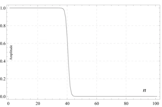
to consider the first term not critical for truncation values N above 2c π, when the energy factor λn

( )

c rapidly approaches zero (an example is shown in

[image:8.595.64.542.83.381.2]

(9)

[image:9.595.211.540.64.282.2]

Figure 7. Eigenvalues λn

( )

c vs. order n for c=20π and ncrit=2c π 40= .

sufficiently large n, the integral

(

0

( ) ( )

)

0

2

, d

t

n t f t ψ c t t

−

∫

tends to zero faster than

the corresponding λn

( )

c at the denominator of the products

( )

2

n n

a λ c . This consideration motivated our work and indirectly highlights again that calculating accurate coefficients an for large n is critical since both overlap

integrals and eigenvalues become very small quantities. This has been a known problem since the 60’s of the last century. The critical aspect is an accurate calculation of ψ_n

( )

c t, , which is now possible [8]. Under the assumption that

the function f t

( )

is initially known in

[

−t t₀,₀

]

, the sum of truncation errors,

computer roundoff and analog to digital conversion errors makes the practical implementation of the proposed iterative approach subject to a total error that has been measured as normalized mean-square error (NMSE) between the original function and the extrapolated signal fe as:

( )

0

2 2

d NMSE

d

e

e t T

i t T e

t T

f t f t t

f f

f f t t

+ − +

− −

= =

∫

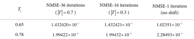
(11)

It is clear from Table 3 that the zero-shift still gives the best results up to the point it is capable to extrapolate correctly (e.g., Te=0.65); increasing N will

extend Te and it will still be the best extrapolation up to that point. However, if

N is a limit, as in practice always is, our shifting method performs better. This

can be interpreted as a consequence of the multiplication by the quantity

(

,

)

n c t T

ψ − _{in (6) which means moving the energy of the LPFs accordingly to}

(10)

[image:10.595.209.539.91.157.2]

Table 3. Normalized mean-square error (NMSE).

e

T NMSE-36 iterations

(T=0.7)

NMSE-16 iterations (T =0.3)

NMSE-1 iteration (no shift)

0.65 7

1.432420 10× − 7

1.432421 10× − 7

1.02351 10× −

0.78 4

1.99422 10× − 4

1.99432 10× − 4

2.28493 10× −

notation in (8). The extrapolation can be optimized by reconstructing the extrapolated function f ti

( )

as concatenation of the known function with segments

of optimum estimates. However, we still observe numerical inaccuracies oc- curring at the points of concatenations, which is presently under investigation.

6. Conclusion

In this paper, we have proposed and implemented a low complexity iterative algorithm for bandlimited signal extrapolation based on orthogonal projections over real-valued eigenvectors: the linear prolate functions. The method is valid for an arbitrary large range of frequencies with immediate applications in signal processing. The main contribution of our work is a theoretical derivation such that given a truncated series (up to a selectable value) of prolate functions, it is possible to extrapolate the bandlimited function (initially known in a limited time interval) elsewhere if each extrapolated portion of the function is subject only to moderate series truncation errors. These errors are controllable by the depth of extrapolation at each iteration. By doing so and with the aim of finding an alternative solution to the initial problem of implementing an accurate summation of infinite terms, we have investigated a property of the signal decomposition formula based on LPFs according to which the integration interval does not need to be symmetric with respect to the origin while time-shifted prolate functions are used in the summation. Also, we have investigated the effects of different sources of errors by implementing and analyzing the iterative algorithm as a generalization of the special case presented in [10]. Our method has shown to outperform concurrent approaches in terms of the normalized mean-square error of the extrapolated signal.

References

[1] Slepian, D. and Pollak, H.O. (1961) Prolate Spheroidal Wave Functions, Fourier Analysis, and Uncertainty—I. The Bell System Technical Journal, 40, 43-63.

https://doi.org/10.1002/j.1538-7305.1961.tb03976.x

[2] Moore, I.C. and Cada, M. (2004) Prolate Spheroidal Wave Functions, an Introduc-tion to the Slepian Series and Its Properties. Applied and Computational Harmonic Analysis, 16, 208-230.

[3] Frieden, B.R. (1971) Evaluation, Design and Extrapolation Methods for Optical Signals Based on Use of the Prolate Functions. Progress in Optics, 9, 311-407. [4] Soman, S. and Cada, M. (2017) Design and Simulation of a Linear Prolate Filter for

(11)

https://www.omicsgroup.org/journals/design-and-simulation-of-a-linear-prolate-fil

ter-for-a-baseband-receiver-2165-7866-1000197.pdf

[5] Papoulis, A. (1975) A New Algorithm in Spectral Analysis and Band-Limited Extrapolation. IEEE Transactions on Circuits and Systems, 22, 735-742.

https://doi.org/10.1109/TCS.1975.1084118

[6] Shi, J., Sha, X., Zhang, Q. and Zhang, N. (2012) Extrapolation of Bandlimited Sig-nals in Linear Canonical Transform Domain. IEEE Transactions on Signal Proces- sing, 60, 1502-1508. https://doi.org/10.1109/TSP.2011.2176338

[7] Zhao, H., Ran, Q.W., Ma, J. and Tan, L.Y. (2010) Generalized Prolate Spheroidal Wave Functions Associated with Linear Canonical Transform. IEEE Transactions on Signal Processing, 58, 3032-3041. https://doi.org/10.1109/TSP.2010.2044609

[8] Cada, M. (2012) Private Communication. Department of Electrical and Computer Engineering, Dalhousie University, Halifax, Canada.

[9] Xiao, H. (2001) Prolate Spheroidal Wave Functions, Quadrature, Interpolation, and Asymptotic Formulae. Ph.D. Dissertation, Department of Computer Science, Yale University,New Haven.

[10] Devasia, A. and Cada, M. (2013) Bandlimited Signal Extrapolation Using Prolate Spheroidal Wave Functions. IAENG International Journal of Computer Science, 40, 291-300.

Submit or recommend next manuscript to SCIRP and we will provide best service for you:

Accepting pre-submission inquiries through Email, Facebook, LinkedIn, Twitter, etc. A wide selection of journals (inclusive of 9 subjects, more than 200 journals)

Providing 24-hour high-quality service User-friendly online submission system Fair and swift peer-review system

Efficient typesetting and proofreading procedure

Display of the result of downloads and visits, as well as the number of cited articles Maximum dissemination of your research work