Munich Personal RePEc Archive
Design of Supply Chain Networks with
Supply Disruptions using Genetic
Algorithm
Taha, Raghda and Abdallah, Khaled and Sadek, Yomma and
El-Kharbotly, Amin and Afia, Nahid
College of International Transport and Logistics, Arab Academy for
Science, Technology and Maritime Transport, Egypt, Faculty of
Engineering, Ain Shams University, Egypt
10 May 2014
1
Design of Supply Chain Networks with Supply Disruptions
using Genetic Algorithm
Raghda Taha ([email protected]), Khaled Abdallah
College of International Transport and Logistics, Arab Academy for Science, Technology and Maritime Transport, Egypt
Yomna Sadek, Amin El-Kharbotly, Nahid Afia Faculty of Engineering, Ain Shams University, Egypt
Abstract
The design of supply chain networks subject to disruptions is tackled. A genetic algorithm with the objective of minimizing the design cost and regret cost is developed to achieve a reliable supply chain network. The improvement of supply chain network reliability is measured against the supply chain cost.
Keywords
Supply chain, Disruptions, Genetic Algorithm
Introduction
Since the early 2000’s, supply chain networks with disruptions have gained a lot of interest in the
scientific research (journal articles, working papers, books, etc.). In the last 15 years, some huge international companies have faced supply disruptions that caused huge losses. Nokia, Ericsson, Toyota, Dole and Chiquita are some examples. Supply disruptions were due to different reasons. Fires, earthquakes, and hurricanes are the most famous examples. The response of the different companies towards the disruptions varied. Therefore, the sizes of the losses also varied. Some were able to recover in weeks. Others stayed for a year until they recovered their original status (Tomlin 2006).
Several definitions have been presented for the supply chain disruptions. Snyder et al. (2012) defined disruptions as “random events that cause a supplier or other element of the supply chain to stop functioning, either completely or partially, for a (typically random) amount of time”.
Literature review
2
Disruptions at the distribution centres were investigated by Azad et al. (2013), and Baghalian et al. (2013). Azad et al. (2013) studied the design problem of a reliable stochastic supply chain network with random disruptions in the location of distribution centres and the transportation modes. The disruption could fail the whole of the capacity, or a fraction of it. The rest of demand can be served by other distribution centres. They solved the problem at two phases; the first is an exact solution method by reformulating the problem as a second-order cone programming model, and the second is a hybrid algorithm combining tabu search and simulated annealing algorithms. Baghalian et al. (2013) developed a stochastic mathematical formulation for designing a network of multi-product supply chains comprising several capacitated production facilities, distribution centres and retailers in markets under uncertainty. The model additionally considered demand-side uncertainties simultaneously.
Facility disruptions were studied by Shukla et al. (2011), Liu et al (2011), and Garcia-Herreros et al. (2013).
Shukla et al. (2011) studied the impact of facility and link failures on a network's performance measures of efficiency and robustness. They incorporated a robustness metric that is based on expected losses incurred due to not meeting demand on time after a disruption has occurred. Their study formulated a mixed integer linear program model with the objective of maximizing both efficiency and robustness. It also evaluates the trade-offs between efficiency and robustness. They found that the resulting supply chain was much more reliable in the long term since the robustness was built into the system without compromising a lot on efficiency.
(Liu 2011) A model regarding the supply chain network under production disruption risk was developed based on the concept of supernetworks and the theory of variational inequalities. The model consists of multiple suppliers and multiple manufacturers, and considers the impact of production disruption risks on the costs, profits, and capacity decisions of the supply chain firms. The variational inequality formulation was used to express the equilibrium conditions of the supply chain network where all decision makers' optimal conditions are simultaneously satisfied. The conditions for the existence of solution and conditions of monotonicity were provided.
Garcia-Herreros et al. (2013) considered decisions on the facility location and the inventory management simultaneously. They proposed a formulation based on a two-stage stochastic programming framework where the scenarios are determined by the possible combinations of facility disruptions. The objective was to minimize the sum of investment cost and the expected cost of distribution during a finite time horizon. The results showed that the proposed formulation generates supply chain designs with the capability to adjust to adverse scenarios. It reflects the savings when disruptions occur in the operation of supply chains.
Qi et al. (2010) were concerned with the supply chain design problem where the system is subject to random supply disruptions that may occur at either the supplier or the retailers. They proved that the cost savings from considering supply disruptions at the supply chain design phase (rather than at the tactical or operational phase) are usually significant.
3
this problem. Their computational simulations revealed very promising results in terms of the quality of solution.
Related studies to the design of supply chains under disruptions were also reviewed. Craighead et al. (2007) focused on how and why one supply chain disruption would be more severe than another. They related the severity of supply chain disruptions (i) to the three supply chain design characteristics of density, complexity, and node criticality and (ii) to the two supply chain mitigation capabilities of recovery and warning.
It is the objective of this research to consider the disruption during the design phase of the supply chain. It is required to find the design of the least cost and the highest reliability under different scenarios of facility disruption, and find the mitigation plan of the least cost simultaneously.
Nomenclature
: Total number of customers c = [1, 2, 3…C]
: Total number of operating distribution centres d = [1, 2, 3…D] : Total number of operating facilities f = [1, 2, 3…F]
: Penalty cost per unit for shortage in customer’s demand : Under capacity cost per unit for un-used capacity in facilities
: Fixed cost of operating distribution centre (d) per planning interval
: Fixed cost of operating facility (f) per planning interval
: Fill rate. It is the minimum percentage of customer demand to be satisfied
: Total capacity of distribution centre (d)
: Total capacity of facility (f)
: Quantities of demand at customer (c)
: Quantities of products produced at facility (f) and transported to distribution centre (d)
: Quantities of product units transported from distribution centre (d) to customer (c)
: Transportation cost of the link between facility (f) and distribution centre (d) plus the
production cost at facility (f) per unit product
: Transportation cost of the link between distribution centre (d) and customer (c) per unit
product
The proposed model:
The proposed model will present first the “basic” case of supply chain network design without disruptions. Afterwards, disruptions are added to the model. It is assumed that a disruption at a facility causes complete failure at the facility. The different mitigation plans are investigated. There are three mitigation plans:
In case of a facility disruption, use over-capacity production from other facilities in the supply chain at a higher cost
In case of a disruption, use out-sourcing at much higher cost from facilities outside the supply chain
4
This paper presents the first plan only, as the other plans are still under investigation.
The assumptions associated with the “basic” model are:
1. The network consists of three echelons; facilities, distribution centres, and customers. 2. The potential facilities and distribution centres have predetermined capacities.
3. The supplier capacity is indefinitely large. 4. Customers’ demands are deterministic.
5. Customer demand should be completely satisfied.
6. All the links between the different echelons are available.
7. Products flow through the network in batches of a pre-determined batch size.
A Genetic Algorithm (GA) is used to generate different designs of the supply chain network from the potential facilities and distribution centres. A binary presentation is used for generating the chromosomes. The chromosome length represents the number of potential facilities and distribution centres. For each gene represent a certain facility or a distribution centre. The zero means that this facility/distribution centre is closed and the one means it is opened. For each design, Integer Linear Programming (ILP) is used to find the optimum links and quantities of products flowing through them with the objective of minimizing the cost. The network of minimum cost is finally detected.
The objective function of the basic model aims at minimizing the total cost. It consists of the fixed cost of facilities and distribution centres, the production cost at the facilities, the transportation cost at the different links, the penalty cost for not satisfying all the demand of the customers, and the cost of operating under the full capacity of the facilities. This is shown in equation (1).
∑
∑
∑ ∑
∑ ∑
∑ ( ∑
)
(∑
∑ ∑
)
(1)
Model constraints:
Capacity constraints for the facilities and the distribution centres are as shown in equations (2)and (3)
∑
(2)
∑
5
Demand satisfaction constraint is as shown in equations (4)
∑
(4)
Balance constraints at the distribution centres are shown in equations (5)
∑
∑
(5)
Non-negative constraints are shown in equation (6)
Integer constraints are shown in equation (7)
Mitigation plan: Over-capacity production- after a disruption occurs
In case of a disruption that causes complete failure at a facility, other facilities in the supply chain should substitute for the missing production by their un-used capacity, and their over-capacity. The quantities that were produced by the disrupted facility will be denoted by
. They are to be transported to the same distribution centres as in the normal case
before disruption.
: Operating facilities as the optimum design in the normal case
: Operating facilities without counting the facility under disruption : Probability that facility (f) will face complete disruption
: Over-capacity of facility (f)
: Quantities that were produced by the disrupted facility and transported to distribution centre (d).
: Quantities that were produced by the un-disrupted facilities and transported to
distribution centre (d) during the normal case. These are fixed values obtained from the ILP of the normal case.
: Quantities produced at facility (f) within its normal capacity and transported to
distribution centre (d) to substitute quantities of disrupted facility.
: Quantities produced at facility (f) from its over-capacity and transported to
distribution centre (d) to substitute quantities of disrupted facility.
: Transportation cost of the link between facility (f) and distribution centre (d) plus
the over-production cost at facility (f) per unit product
,c (6)
6
In this case, ILP will be applied again to minimize the “recovery cost”; it is the extra cost paid due to production at the un-disrupted facilities. Equation (8) is the new objective function to be minimized.
∑ ∑
∑ ∑
(8)
Facility capacity constraints are the only constraints in this ILP optimizations. They include both normal production and over-production capacities as in (9) and (10).
∑
(9)
∑
(10)
The total cost shown in equation (11) is the design cost and regret cost. The design cost is calculated in terms of the cost of the basic case (1) , while the regret cost is the cost incurred due to disruptions in this case the recovery cost(8). This cost is multiplied by the probability of the disruption at each of the operating facilities.
( ∑
) (11)
.
For each network design the genetic algorithm generates, the “basic” cost as well as the total cost
are calculated.
Several experiments were carried to test the proposed model, and to examine the behaviour of the supply chain under disruptions. These experiments are shown in the following section.
Computational results
A set of numerical experiments were conducted in order to evaluate the proposed model. For small instances the model was coded using Microsoft excel with macro enabled on a computer core i7 ,1.9 GHz with 8GB Ram.
7 Table 1 Data set for numerical example
Parameter Value
Production cost P = 10 unit cost
Transportation cost 0.1 × P
Under-capacity cost 0.5 × P
Penalty cost 3 × P
Over-capacity cost 1.5 × P
Facility fixed cost Max facility capacity × P Distribution centres capacity 300
Distribution centres fixed cost (Max DC capacity × P)/6
Demand 1000 unit
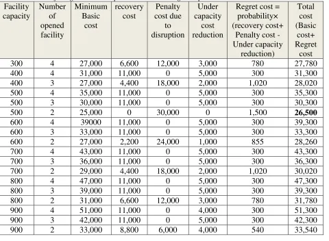
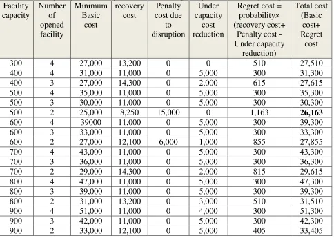
The problem size of the generated test problem is considered relatively small. Accordingly, the number of all feasible chromosomes is limited so for this problem all feasible chromosomes where tested in the initial population. The results are given in table 2 where no mitigation plan is applied and in table 3 where over-capacity production is used as a mitigation plan. The recovery cost is calculated for each scenario. Moreover, a penalty cost is calculated if the demand is not satisfied in case of disruptions. Since the excess capacity of other facilities that is not subjected to disruption will be used to satisfy the disrupted facility a reduction in the under-capacity cost must be considered.
Table 2 Results of the generated test problem with no mitigation plan Facility capacity Number of opened facility Minimum Basic cost recovery cost Penalty cost due to disruption Under capacity cost reduction
Regret cost = probability× (recovery cost+
Penalty cost - Under capacity reduction) Total cost (Basic cost+ Regret cost
300 4 27,000 6,600 12,000 3,000 780 27,780
400 4 31,000 11,000 0 5,000 300 31,300
400 3 27,000 4,400 18,000 2,000 1,020 28,020
500 4 35,000 11,000 0 5,000 300 35,300
500 3 30,000 11,000 0 5,000 300 30,300
500 2 25,000 0 30,000 0 1,500 26,500
600 4 39000 11,000 0 5,000 300 39,300
600 3 33,000 11,000 0 5,000 300 33,300
600 2 27,000 2,200 24,000 1,000 855 28,260
700 4 43,000 11,000 0 5,000 300 43,300
700 3 36,000 11,000 0 5,000 300 36,300
700 2 29,000 4,400 18,000 2,000 1,020 30,020
800 4 47,000 11,000 0 5,000 300 47,300
800 3 39,000 11,000 0 5,000 300 39,300
800 2 31,000 6,600 12,000 3,000 780 31,780
900 4 51,000 11,000 0 4,000 300 51,300
900 3 42,000 11,000 0 5,000 300 42,300
[image:8.612.68.548.377.729.2]8
[image:9.612.69.553.153.498.2]The capacities of the potential facilities is varied to generate different instances of the problem. Each problem is solved with four disruption scenarios where each scenario consider the closure of one facility. The probability of each scenario is 0.05.
Table 3 Results of the generated test problem with Over-capacity production as mitigation plan Facility capacity Number of opened facility Minimum Basic cost recovery cost Penalty cost due to disruption Under capacity cost reduction
Regret cost = probability× (recovery cost+
Penalty cost - Under capacity reduction) Total cost (Basic cost+ Regret cost
300 4 27,000 13,200 0 0 510 27,510
400 4 31,000 11,000 0 5,000 300 31,300
400 3 27,000 14,300 0 2,000 615 27,615
500 4 35,000 11,000 0 5,000 300 35,300
500 3 30,000 11,000 0 5,000 300 30,300
500 2 25,000 8,250 15,000 0 1,163 26,163
600 4 39000 11,000 0 5,000 300 39,300
600 3 33,000 11,000 0 5,000 300 33,300
600 2 27,000 12,100 6,000 1,000 855 27,855
700 4 43,000 11,000 0 5,000 300 43,300
700 3 36,000 11,000 0 5,000 300 36,300
700 2 29,000 14,300 0 2,000 815 29,615
800 4 47,000 11,000 0 5,000 300 47,300
800 3 39,000 11,000 0 5,000 300 39,300
800 2 31,000 13,200 0 3,000 510 31,510
900 4 51,000 11,000 0 4,000 300 51,300
900 3 42,000 11,000 0 5,000 300 42,300
900 2 33,000 12,100 0 5,000 405 33,405
Conclusion and recommendation of future work
From the computational results it can be concluded that the regret cost and recovery cost represent a significant value of the total cost and should be included from the design phase. Also in case of networks that are subjected to higher probabilities of disruptions the regret cost will increase significantly and it might be better to design network which is not optimal in the basic case but it has the minimum total cost including both design cost and regret cost. In case of the over production mitigation plan in most of the cases all the demand was satisfied. Also the under capacity cost reduction was applied. In all instances, applying the over-capacity production mitigation plan obtained better solution with less total cost than in case of disruption with no mitigation plan applied.
Future work will include the investigation of the other two mitigation plans;
9
Before a disruption occurs, build up inventory to be used in case of disruptions.
It can also include other sources of disruptions that can be considered separately or simultaneously; e.g. disruption at distribution centres, or disruption in transportation. Disruptions may cause partial or full failure.
Another type of disruptions is demand disruptions. An important feature of demand disruption is that it can either be an increase or a decrease in the demand.
Bibliography
Azad, N., Davoudpour, H.,Saharidis, G.K.D., Shiripour, M. 2013. A new model to mitigating random disruption risks of facility and transportation in supply chain network design. International Journal of Advanced Manufacturing Technology:1-18
Baghalian, A., Rezapour, S.,Farahani, R.Z. 2013.Robust supply chain network design with service level against disruptions and demand uncertainties: A real-life case. European Journal of Operational Research
227(1): 199-215
Chen, T.-G., Ju, C.-H. 2013.A novel artificial bee colony algorithm for solving the supply chain network design under disruption scenarios. International Journal of Computer Applications in Technology 47(2): 289-296.
Craighead, C.W., Blackhurst, J., Rungtusanatham, M.J.,Handfield, R.B. 2007. The severity of supply chain disruptions: Design characteristics and mitigation capabilities. Decision Sciences 38(1): 131-156
Garcia-Herreros, P.,Grossmann, I.E., Wassick, J. 2013. Design of supply chains under the risk of facility disruptions. Computer Aided Chemical Engineering32: 577-582
Lawrence, V. S., Atan, Z., Peng, P., Rong, Y., Schmitt, A. J., Sinsoysal, B. 2010. OR/MS Models for Supply Chain Disruptions: A Review. SSRN eLibrary.
Liu, Z.-G. 2011.Supply chain network design under production disruption risk. Shanghai Ligong Daxue
Xuebao/Journal of University of Shanghai for Science and Technology33( 3): 264-267+278
Qi, L., Shen, Z.-J.M., Snyder, L.V. 2010. The effect of supply disruptions on supply chain design decisions. Transportation Science 44 (2): 274-289
Shukla, A., Lalit, V.A.,Venkatasubramanian, V. 2011. Optimizing efficiency-robustness trade-offs in supply chain design under uncertainty due to disruptions. International Journal of Physical Distribution
and Logistics Management41(6):623-646