Testing for Dornbusch and Delayed Overshooting: Setting the Record Straight

http://www.scirp.org/journal/tel ISSN Online: 2162-2086

ISSN Print: 2162-2078

DOI: 10.4236/tel.2019.95096 Jun. 20, 2019 1489 Theoretical Economics Letters

Testing for Dornbusch and Delayed

Overshooting: Setting the Record Straight

John Pippenger

Department of Economics, University of California, Santa Barbara, CA, USA

Abstract

Several articles report impulse responses from policy shocks to exchange rates that never have a significant change in sign and converge to zero. Most claim that such impulse responses support some form of Dornbusch or delayed overshooting. This article shows that such impulse response functions reject overshooting from policy shocks to exchange rates. It also shows that, with-out additional information, such impulse responses provide no credible evi-dence for or against Dornbusch or delayed overshooting; that is overshooting from the policy variable itself to the exchange rate. Finally it shows that the one article that provides enough information for an appropriate test of such overshooting rejects it.

Keywords

Exchange Rates, Impulse Response, Step Response, Overshooting, Vector Autoregression

1. Introduction

Table 1 lists the articles that use impulse responses to test for how exchange

rates respond to monetary policy starting with the seminal [1].1

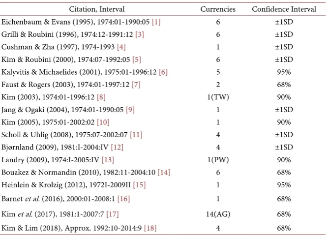
Table 1 provides the citation, interval covered, number of currencies analyzed and confidence interval. Confidence intervals are important because many ar-ticles use unusually narrow confidence intervals, e.g. 68% rather than the custo-mary 90% or 95%. As a result, estimates that articles claim are “significant” may not be significant at customary levels.

With the exceptions of [1] and [4], the articles in Table 1 claim to find evi-dence of either Dornbusch overshooting or a delayed version of Dornbusch over-shooting. For example [12] claims to find evidence of Dornbusch overshooting; 1_{See [2]for a review of the earlier literature on overshooting.}

How to cite this paper: Pippenger, J. (2019) Testing for Dornbusch and Delayed Overshooting: Setting the Record Straight. Theoretical Economics Letters, 9, 1489-1506. https://doi.org/10.4236/tel.2019.95096

Received: March 29, 2019 Accepted: June 17, 2019 Published: June 20, 2019

Copyright © 2019 by author(s) and Scientific Research Publishing Inc. This work is licensed under the Creative Commons Attribution International License (CC BY 4.0).

[image:2.595.207.540.87.327.2]

DOI: 10.4236/tel.2019.95096 1490 Theoretical Economics Letters Table 1. Testing for overshooting: The literature.

Citation, Interval Currencies Confidence Interval Eichenbaum & Evans (1995), 1974:01-1990:05 [1] 6 ±1SD Grilli & Roubini (1996), 1974:12-1991:12 [3] 6 ±1SD Cushman & Zha (1997), 1974-1993 [4] 1 ±1SD Kim & Roubini (2000), 1974:07-1992:05 [5] 6 ±1SD Kalyvitis & Michaelides (2001), 1975:01-1996:12 [6] 5 95% Faust & Rogers (2003), 1974:01-1997:12 [7] 2 68% Kim (2003), 1974:01-1996:12 [8] 1(TW) 90% Jang & Ogaki (2004), 1974:01-1990:05 [9] 1 ±1SD Kim (2005), 1975:01-2002:02 [10] 1 90% Scholl & Uhlig (2008), 1975:07-2002:07 [11] 4 ±1SD Bjørnland (2009), 1981:I-2004:IV [12] 4 ±1SD Landry (2009), 1974:I-2005:IV [13] 1(PW) 90% Bouakez & Normandin (2010), 1982:11-2004:10 [14] 6 68% Heinlein & Krolzig (2012), 1972I-2009II [15] 1 95% Barnet et al. (2016), 2000:01-2008:1 [16] 1 68% Kim et al. (2017), 1981:1-2007:7 [17] 14(AG) 68% Kim & Lim (2018), Approx. 1992:10-2014:9 [18] 4 68%

Notes: TW: Trade weighted exchange rate; PW: Population weighted exchange rate; AG: Aggregated.

[3] claims to find evidence of a delayed version of such overshooting with a short delay while [7] and [14] claim to find evidence of delayed overshooting with a longer delay.2

The models in Table 1 associated with “Dornbusch” overshooting, or a de-layed version of such overshooting, are not directly related to the Dornbusch overshooting model in [19]. Money is not the policy variable; they do not as-sume perfect foresight or rational expectations and they usually do not asas-sume uncovered interest parity.

They also are particularly susceptible to specification search. As [20]points out in “Let’s Take the Con Out of Econometrics”, specification search, which invali-dates traditional statistical tests, is endemic. The articles in Table 1 potentially suffer from all the standard pitfalls of specification search described in [20] plus the additional pitfalls created by the restrictions necessary to estimate VAR models.3 _{One response to specification search is to show that the same model}

holds across time and space, which the overshooting literature does not do. Pol-icy variables, models and restrictions change across the articles in Table 1.

When someone submits a paper to a journal that includes estimating a model, 2_{[7] is less supportive of overshooting than most of the subsequent literature assumes. In their} sum-mary on page 1406 they point out that the delayed overshooting results are quite sensitive to dubious assumptions and that the share of exchange rate volatility due to US monetary shocks is not sharply identified; reasonable estimates go from zero to over half. We interpret this to mean that one rea-sonable interpretation of the evidence is that policy shocks contribute nothing to the volatility of exchange rates, which of course rejects overshooting from policy shocks to exchange rates.

DOI: 10.4236/tel.2019.95096 1491 Theoretical Economics Letters

they implicitly certify that the model makes economic sense and that the eco-nometrics is appropriate, e.g., there is no specification search. This journal, like most, has an ethical code that prohibits the submission of articles that use data fraudulently. When a journal publishes an article, peer review implicitly re-certifies the paper. This article takes that certification as valid. It assumes that the models

in Table 1 make economic sense and that the econometrics produces reliable

es-timates of impulse response functions that can be used to produce step response functions and test for overshooting. It also assumes that there was no specifica-tion search. Taking all this for granted, it then shows that the impulse response functions reported in Table 1 reject overshooting from policy shocks to ex-change rates and that, without more information, the articles tell us nothing useful about overshooting from policy variables themselves to exchange rates.

There are at least three additional problems with the articles that claim to find evidence of overshooting: 1) Unlike the Dornbusch overshooting model, no ar-ticle provides a benchmark that shows what the volatility of exchange rates would be without overshooting. Without a benchmark, unless one is willing to attribute all exchange-rate volatility created by policy shocks to overshooting, there is no way to measure how much, if any, of the total volatility in exchange rates is due to overshooting. 2) Impulse responses from policy shocks, which are I(0), to exchange rates, which are I(1), reported in Table 1 do not explain the unit root in exchange rates. 3) Only one article in Table 1 defines what it means by “Dornbsuch overshooting” [7]. It makes it clear that such overshooting is the result of a permanent increase in money. Only one article defines what it means by “delayed” overshooting [17], but it fails to make it clear whether or not the “monetary contraction” is permanent or temporary. For clarity, we define what we mean by “Dornbusch” and “delayed” overshooting and point out how this overshooting differs from the “policy” responses in Table 1.

The next section reviews impulse and step responses and how they relate to overshooting in a framework like the overshooting model in [19]. It also points out the special nature of Dornbusch overshooting and the delayed version of that overshooting. Section 3 extends the discussion to VAR and considers two special conditions where impulse response functions from policy shocks to ex-change rates provide information that can be used to test for overshooting from policy variables to exchange rates. Neither is relevant.

Section 4 shows that, when one excludes these conditions, impulse responses from policy shocks to exchange rates, and their corresponding step responses, are, without more information, essentially useless as tests for overshooting from policy variables themselves to exchange rates.

2. Impulse Responses, Step Responses and Overshooting

DOI: 10.4236/tel.2019.95096 1492 Theoretical Economics Letters

tion between those responses and overshooting. Equations (1) and (2) describe a simple discrete version of the deterministic Dornbusch model in [19]. The next section extends the discussion to VAR.

s(t), p(t) and m(t) represent logs of exchange rates, price levels and money respectively. Prices depend on money while exchange rates depend on prices and money. Money in the Dornbusch overshooting model is not just econometrically exogenous, it is determined outside the model. Throughout this section we as-sume that m(t) is determined outside the model. We drop that assumption later.

( )

1

(

1

)

2

(

2

)

3

(

3

)

p t =

β

m t− +

β

m t− +

β

m t− (1)

( )

( )

( )

(

)

(

)

(

)

(

)

(

)

0 0 1 2

3 4 5

1 2

3 4 5

s t a p t b m t b m t b m t

b m t b m t b m t

= + + − + −

+ − + − + − (2)

with all 0≤

β

_i <1.0 and their sum equal to 1.0, prices respond gradually to

money and the quantity theory holds in the long run as in [19]. With a0 equal to

1.0 and the sum of the bi equal to zero, purchasing power parity (PPP) holds in

the long run as in the Dornbusch overshooting model.

We begin with an impulse response function where the input is m(t) and the output is s(t).

( )

m s,

( ) ( )

s t =h L m t (3)

In general, hm s,

( )

L =bm

( ) ( )

L as L where as(L) and bm(L) are polynomials in the lag operator L. Using (1) and (2) as an example,

( )

(

) (

)

2

(

)

3 4 5

, 0 1 0 1 2 0 2 3 0 3 4 5

m s

h L =b + b +a

β

L+ b +a

β

L + b +a

β

L +b L +b L.

Discrete impulse response functions like hm,s(L) describe how “outputs” like

s(t) respond to a unit pulse in “inputs” like m(t). A unit pulse is zero for all t be-fore t = 0, equals 1.0 when t = 0, and is zero for all subsequent t. There is often an implicit assumption that, before t = 0, both s(t) and m(t) have been in a steady state equilibrium with s(t) and m(t) equal to zero.

With a typical inverted “U” hm,s(L) like

2 3 4 5

0.1 0.3+ L+0.6L +0.3L +0.075L +0.025L , a unit pulse in m(t) produces the

following s(t): s(−1)= 0, s(0)= 0.1, s(1)= 0.3, s(2)= 0.6, s(3)=0.3, s(4)= 0.075,

s(5) = 0.025, with all subsequent s(t) equal to zero.

Discrete step response functions describe how “outputs” like s(t) respond to a unit step in “inputs” like m(t). A unit step is zero for all t before t = 0 and equals 1.0 for t = 0 and all subsequent t. Once again there often is an implicit assump-tion that before the unit step the system is in equilibrium with s(t) and m(t) equal to zero. When Dornbusch describes overshooting in [19] he describes how

s(t) responds to a permanent one unit increase in m(t). That is he uses a step re-sponse from m(t) to s(t), not an impulse response from m(t) to s(t), to describe how exchange rates overshoot in response to a permanent increase in money. Like Dornbusch, we use step responses, not impulse responses, to describe overshooting

in-DOI: 10.4236/tel.2019.95096 1493 Theoretical Economics Letters

vestment by using an impulse response function. They would use the income multiplier with respect to investment, i.e. the step response from autonomous investment to income.

If hm,s(L) is the impulse response from m(t) to s(t), then the corresponding

step response gm,s(L) is the sum of that impulse response. That is

( )

( )

, ,

0

N

N K

m s m s

K

g L h L

=

=

∑

_or g_{m s,}

( )

L =h_{m s,}

( )

L ∆. Looked at from the point of

view of the step response, hm s,

( )

L = ∆gm s,

( )

L . An impulse response function is the change in the corresponding step response function.

With hm,s(L)the inverted “U” of 0.1 0.3+ L+0.6L2+0.3L3+0.075L4+0.025L5,

the corresponding step response or gm,s(L)is

2 3 4 5

0.1 0.4+ L+1.0L +1.3L +1.375L +1.4L + + 1.4LN. A unit step in m(t)

pro-duces the following s(t): s(−1) = 0.0, s(0) = 0.1, s(1) = 0.4, s(2) = 1.0, s(3) = 1.3,

s(4) = 1.375, s(5) = 1.4 with all subsequent s(t) equal to 1.4.

Dornbusch uses a step response to describe overshooting for good reason; the relationship between impulse responses and overshooting is tenuous. Over-shooting in his context is normally defined, and best discussed, in terms of step responses, not impulse responses. This article uses the following simple defini-tion of generic overshooting that assumes a positive response: There is over-shooting when some transient response to a unit step input is greater than the steady-state response.5 _{This is the definition implicit in Table 1, but those}

ar-ticles never mention step response functions or even the response of exchange rates to permanent changes in “inputs”. They only report impulse responses and they never discuss how those impulse responses are related to “overshooting”.

Our simple definition of overshooting defines the relation between impulse responses and overshooting. If there is overshooting, the corresponding impulse response must change sign. If it does not change sign, there is no overshooting. But a change in the sign of an impulse response does not imply overshooting. A change in the sign of the corresponding impulse response is a necessary, but not sufficient, condition for overshooting from the input to the output.

[7] provides the only “definition” of Dornbusch overshooting in Table 1. It essentially defines Dornbusch overshooting as follows: there is Dornbusch over-shooting when a unit step in the domestic money stock produces a maximum transient response in the exchange rate at impact that exceeds a steady state re-sponse that is positive. This definition differs slightly from the one implicit in the Dornbusch overshooting model in two ways: first money is determined out-side the model and second steady state responses to unit steps are one because PPP holds in the long run.

DOI: 10.4236/tel.2019.95096 1494 Theoretical Economics Letters

unit pulse.

We assume that delayed overshooting is the same as “Dornbusch” overshoot-ing except that the maximum transient response is after impact; how long after is unclear.

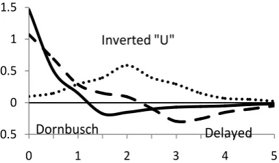
Continuing with our simple Dornbusch model, Figure 1 illustrates three step

responses labeled “Dornbusch” “Delayed” and “Inverted U” while Figure 2 illu-strates the corresponding impulse responses. The input in Figure 1 is a unit step in money with the exchange rate as the output. The input in Figure 2 is a unit pulse in money with the exchange rate as the output.

The solid gm,s(L) in Figure 1 labeled “Dornbusch” is easily recognized as

Dornbusch overshooting. The maximum transient response to the unit step is at impact, it is greater than the steady state response and the steady state response is 1.0.

The steady state response of 1.0 for this gm,s(L) provides a benchmark for

measuring the amount of overshooting. For the solid step response in Figure 1

labeled “Dornbusch”, all transient responses greater than 1.0 represent “over-shooting”. Articles in Table 1 never mention benchmarks. As pointed out earlier, without them all they can do is determine the amount of the variability in s(t) attributable to policy shocks, not the amount attributable to overshooting.

The dashed gm,s(L) labeled “Delayed” in Figure 1 illustrates a delayed version

of Dornbusch overshooting. The maximum transient response is after impact, it is greater than the steady state response and the steady state response is 1.0. Once again all transient responses greater than 1.0 represent “overshooting”.

We will return to the dotted gm,s(L) labeled Inverted “U” in Figure 1 after

considering the impulse responses associated with the Dornbusch and Delayed overshooting in Figure 1.

Figure 2 describes the impulse responses corresponding to the step responses in Figure 1. The impulse response labeled “Dornbusch” is positive at impact and then immediately turns negative as required by the fact that an impulse response is the change in the corresponding step response. The impulse response labeled “Delayed” is initially positive and then turns negative after t equals 2. Again this pattern is the result of the fact that an impulse response is the change in the

Figure 1. Step response functions.

0 0.5 1 1.5 2

0 1 2 3 4 5

[image:7.595.249.500.71.216.2]

DOI: 10.4236/tel.2019.95096 1495 Theoretical Economics Letters Figure 2. Impulse response functions.

corresponding step response. These impulse responses for Dornbusch or delayed overshooting look nothing like the “U” or inverted “U” shaped impulse res-ponses reported in Table 1 that articles claim support Dornbusch or delayed overshooting.

Like estimated impulse responses from “policy shocks” to exchange rates re-ported in Table 1, the dotted “Inverted U” hm,s(L) in Figure 2 does not change

sign and converges to zero. Since the corresponding step response in Figure 1 is the summation of the inverted U in Figure 2, that step response rises steadily to a new steady state. There is no overshooting because no transient response to the unit step is greater than the steady state response.

Although impulse responses from policy shocks to exchange rates in Table 1

are from more complex systems, the basic point still holds. Impulse response functions that do not change sign reject overshooting from the input to the out-put.

3. VAR

At the beginning of the VAR overshooting literature, [1] introduces a policy re-sponse function: a regression like (4) in a VAR model where v(t) is the policy variable itself.

( )

( )

t

( )

v t =

ζ

Ω +e t (4)

The literature calls a unit pulse in e(t) a “policy shock” or an “innovation” in monetary policy. But giving it those names does not change what it is, simply the error tem in a regression. Note that e(t) must have the same dimension as v(t). It cannot be interpreted as the change in v(t).

When articles in Table 1 claim to find evidence of exchange rate overshooting, they base that claim on impulse response functions from e(t) to the log of the exchange rate s(t) that do not have a statistically significant change in sign and converge to zero. As pointed out above, such impulse response functions reject

overshooting from e(t) to s(t).

After listing some orthogonal conditions and caveats, [1] uses impulse res-ponses from e(t) to s(t) to test for overshooting. At this point the focus of the

-0.5 0 0.5 1 1.5

0 1 2 3 4 5

Inverted "U"

DOI: 10.4236/tel.2019.95096 1496 Theoretical Economics Letters

overshooting literature shifts away from overshooting from m(t) to s(t) as in [19]

to overshooting from e(t) to s(t) and from permanent changes in inputs, i.e. unit steps as in [19], to temporary changes in inputs, i.e. unit pulses.

Unfortunately [1] never discusses how impulse response functions might be used to test for overshooting from e(t) to s(t). Later articles follow their lead and use impulse responses from e(t) to s(t), but they are less careful about interpret-ing those impulse responses. While [1] correctly interprets impulse responses from e(t) to s(t) that do not change sign as evidence of a persistent response to policy shocks, except for [4], later articles misinterpret such impulse responses as support for overshooting from e(t) to s(t).

Contrary to claims made by almost all the subsequent overshooting literature,

[1] never claims to find evidence of overshooting.6 _{The concluding section of [1]}

clearly states that it finds strong evidence that contractionary policy shocks lead to persistent exchange rate appreciation. There is no mention of overshooting.

Step responses from policy variables themselves to exchange rates provide the best way to test for some form of Dornbusch overshooting. However there are two special conditions where VAR impulse response functions alone can provide useful information. One condition is when an impulse response from a policy shock e(t) to a policy variable v(t), i.e. h_{e v,}e

( )

L , equals 1.0. In that case, a unit pulse in e(t) produces a unit pulse in the policy variable v(t). As a result, the im-pulse response from e(t) to s(t) can be interpreted as the impulse response from the policy variable v(t) to the exchange rate s(t) or h_ve,_se

( )

L . In that case v

e_{(t) is}

effectively determined outside the model and the corresponding step response,

( )

,

e e

v s

g L , provides a test for overshooting.

Some reported impulse responses from policy shocks to policy variables are close to 1.0 and a unit pulse in e(t) would produce something close to a unit pulse in the policy variable. But corresponding g_ve_,se

( )

L reject overshooting

because no transient response is greater than the steady-state response.

The other condition is when he v,e

( )

L equals 1/Δ. In that case, a unit pulse in

the policy shock e(t) produces a unit step in the policy variable v(t). In this spe-cial case, the impulse response from e(t) to s(t), h_{e s,}e

( )

L , can be interpreted as

the step response from the policy variable to the exchange rate or g_ve_,se

( )

L . But

this condition is inconsistent with the evidence. Reported h_{e v,}e

( )

L in articles

claiming to support some version of Dornbusch overshooting converge to something that is not statistically different from zero, usually within a few months. See for example Figure 2 in [7].

DOI: 10.4236/tel.2019.95096 1497 Theoretical Economics Letters

such h_{e s,}e

( )

L might be misinterpreted as support for overshooting. If anyone

can suggest a valid interpretation, we would like to know what it is.

3.1.

h

_{e v,}e

( )

L

Chris Sims pointed out to us that, if h_{e v,}e

( )

L rise over time and converge to

some value significantly greater than zero in the steady state, then it might be possible to interpret h_{e s,}e

( )

L as the response of s(t) to something like a unit

step in ve_{(t). In that case the typical inverted “U” shaped}

( )

,e

e s

h L found in the literature might imply delayed overshooting from the policy variable to the ex-change rate. But this possibility is inconsistent with the evidence. Essentially all reported h_{e v,}e

( )

L converge to something that is not significantly different from

zero, usually within a few months.

3.2.

h

_{e s,}e

( )

L

as

g

_{e s,}e

( )

L

There is a strong possibility that several articles interpret h_{e s,}e

( )

L as though

they were g_{e s,}e

( )

L . For example, [3] appears to interpret the impulse response

from e(t) to s(t) as though it were the step response from e(t) to s(t). They say that the impact appreciation is not followed by persistent appreciation and that after impact the exchange rate starts to depreciate quite quickly.

If they were describing a step response from e(t) to s(t), i.e. g_{e s,}e

( )

L , it would

support overshooting from e(t) to s(t). But they are describing an impulse re-sponse from a policy shock to an exchange rate, i.e. an h_{e s,}e

( )

L , that does not

have a significant change in sign. Such impulse response functions reject over-shooting from e(t) to s(t).

3.3. VAR is Special

Another possibility is that h_{e s,}e

( )

L estimated by VAR are special. They

some-how can be interpreted as g_{e s,}e

( )

L . We use RATS to debunk that possibility.

We use IMPULSE.PRG from RATS to estimate the following three equation model describing Dornbusch overshooting using a Choleski decomposition. To keep the model relatively simple, as in [19]m(t) is effectively determined outside the model because h_{e m,} e

( )

L equals 1. As in [19], the quantity theory and PPP

hold in the long run.

( ) ( )

m t =e t (5)

( )

0.1

( )

0.6

(

1

)

0.3

(

2

)

1 2

( )

p t = m t + m t− + m t− +e (6)

( )

( )

(

)

(

)

(

)

(

)

(

)

( )

( )

1.4 0.8 1 0.45 2 0.075 3 0.05 4 0.025 5 2

s t m t m t m t m t

m t m t p t e t

= − − − − − −

− − − − + + (7)

where e(t), e1(t) and e2(t) are orthogonal white noise error terms by construc-tion. Ignoring the error terms, the deterministic g_{m s,}e

( )

L for this model

DOI: 10.4236/tel.2019.95096 1498 Theoretical Economics Letters

Replacing (6) and (7) with (8) and (9) produces the delayed overshooting in

Figure 1 and Figure 2, where again the quantity theory and PPP hold in the

long run.

( )

0.1

( )

0.6

(

1

)

0.3

(

2

)

1 2

( )

p t = m t + m t− + m t− +e (8)

( )

( )

(

)

(

)

(

)

(

)

(

)

( )

( )

1.0 0.3 1 0.2 2 0.3 3 0.15 4 0.05 5 2

s t m t m t t m t

m t m t p t e t

= − − − − − −

− − − − + + (9)

There also is an example that produces the inverted “U” described above.

Figure 3 describes the three simulated step responses from e(t) to s(t) and

Figure 4 the corresponding simulated impulse responses.

VAR impulse responses are conventional impulse response functions. One cannot interpret a VAR impulse response from a policy shock to an exchange rate as though it were a step response from e(t) to s(t).

3.4. Unit Root

This misinterpretation is similar to the previous one. Somehow a unit root in s(t) transforms he s,e

( )

L into ge s,e

( )

L . We continue to assume that m(t) is

statio-nary for two reasons: First common policy variables like short-term interest rates, short-term interest rate differentials and NBRX are likely to be stationary. Second reported h_{e v,}e

( )

L imply that v

e_{(t) are stationary because the}

_{( )}

,e

e v

h L converge to zero.

Equations (10) to (12) describe a simple VAR model with Dornbusch over-shooting where m(t) is stationary and determined outside the model, but s(t) has a unit root because p(t) has a unit root.

( ) ( )

m t =e t (10)

( )

1.0

(

1

)

1 2

( )

p t = p t− +e (11)

( )

( )

(

)

(

)

(

)

(

)

(

)

( )

( )

1.5 0.2 1 0.15 2 0.075 3 0.05 4 0.025 5 2

s t m t m t t m t

m t m t p t e t

= − − − − − −

− − − − + + (12)

Changing Equation (12) to Equation (13) changes the model to one with de-layed overshooting.

( )

( )

(

)

(

)

(

)

(

)

(

)

( )

( )

1.1 0.3 1 0.1 2 0.3 3 0.15 4 0.05 5 2

s t m t m t m t m t

m t m t p t e t

= + − + − − −

− − − − + + (13)

Changing Equation (13) to Equation (14) changes the model to one with an inverted “U”.

( )

( )

(

)

(

)

(

)

(

)

(

)

( )

( )

0.1 0.3 1 0.6 2 0.3 3 0.15 4 0.025 5 2

s t m t m t m t m t

m t m t p t e t

= + − + − + −

+ − + − + + (14)

Figure 5 shows the simulated step responses from e(t) to s(t), which are simi-lar to those in Figure 1 from m(t) to s(t). Figure 6 shows the simulated impulse responses, which are close to those in Figure 2. A unit root in s(t) does not change h_{e s,}e

( )

L into g_{e s,}e

( )

L .

7

7_{Unit roots can introduce bias into estimates of}

( )

,e e s

[image:11.595.267.475.73.190.2] [image:11.595.270.476.224.339.2]

DOI: 10.4236/tel.2019.95096 1499 Theoretical Economics Letters Figure 3. Simulated VAR step responses.

Figure 4. Simulated VAR impulse responses.

Figure 5. Simulated step responses: Unit root.

Figure 6. Simulated impulse responses: Unit root.

3.5. Redefinition

There is generic overshooting when some transient response to a unit step in the input is greater than the steady-state response of the output. It is possible that

0 0.5 1 1.5 2

0 1 2 3 4 5

Inverted "U" Delayed Dornbusch

-2.5 -1.5 -0.5 0.5 1.5

0 1 2 3 4 5

Inverted "U"

Delayed Dornbusch

0 0.5 1 1.5 2

0 1 2 3 4 5

Inverted "U" Delayed Dornbusch

-0.5 0 0.5 1 1.5

0 1 2 3 4 5

Inverted "U"

[image:11.595.271.478.375.490.2] [image:11.595.273.477.525.644.2]

DOI: 10.4236/tel.2019.95096 1500 Theoretical Economics Letters

some articles implicitly redefined overshooting. They replace the unit step with a unit pulse. This redefinition violates the definition implicit in [19].

3.6. Rational Expectations

In models with rational expectations, white noise errors or “innovations” represent “information” that changes the output of the model permanently. Al-though the authors in Table 1 do not generally claim that expectations are ra-tional in their models, some may interpret policy shocks as information about the policy variable that affects the exchange rate permanently.

While unit steps in e(t) might be interpreted as “information”, unit pulses are difficult to interpret as “information”. As long as the relationship described by

( )

,e

e s

h L is stable, a unit pulse in e(t) does not change the steady state value of

s(t).8 _{The new steady state must be the same as the original steady state.}

3.7. Policy Shocks as Changes in Policy Variables

Some articles probably interpret “policy shocks”, or e(t), as changes in the policy variable itself, or Δv(t). Misinterpreting e(t) as Δv(t) would help explain why so many articles in Table 1 appear to interpret h_{e s,}e

( )

L as though they were

( )

,e

e s

g L .

If one could interpret e(t) as Δv(t),then one could write

( )

_,e

( ) ( )

e

e s

s t =h L e t

as

( )

,e

( ) ( )

e

e s

s t =h L ∆v t , which would imply that the impulse response from e(t)

to s(t), h_{e s,}e

( )

L ,was the step response from v(t) to s

e_{(t), i.e.}

_{( )}

,e

v s

g L . In that case the inverted “U” h_{e s,}e

( )

L reported in Table 1 would support delayed

overshooting. But policy shocks are not Δv(t). As pointed out above, e(t) must have the same dimension as v(t) in Equation (4).

To summarize, articles in Table 1 that claim to find evidence of exchange-rate overshooting appear to base that claim on impulse response functions from pol-icy shocks to exchange rates that have no significant change in sign and con-verge to zero. But such impulse response functions reject overshooting and we can find no way to explain how they might support overshooting. In the next section we extend our search for some way to reconcile the claims for over-shooting with the evidence reported in Table 1.

4. Another Approach

The previous section assumes that when articles in Table 1 claim to find evi-dence of “Dornbusch” overshooting or a delayed version of such overshooting, they base that claim on the impulse response function from policy shocks to ex-change rates or h_{e s,}e

( )

L . But Dornbusch overshooting is from his policy

varia-ble m(t) to the exchange rate, not from some “policy shock” to the exchange rate. In this section we consider the possibility that claims of overshooting refer to how policy variables themselves, v(t), affect exchange rates, s(t).

DOI: 10.4236/tel.2019.95096 1501 Theoretical Economics Letters

Without more information, the h_{e s,}e

( )

L reported in Table 1 tell us nothing

useful about overshooting from v(t) to s(t). Without additional information, it is impossible to obtain the step response functions from policy variables them-selves to exchange rates necessary to test for Dornbusch overshooting or a de-layed version of such overshooting.

We illustrate this point first by showing how h_{e s,}e

( )

L can appear to imply

delayed overshooting from e(t) to s(t) when there is no overshooting from m(t) to s(t). Then we show how h_{e s,}e

( )

L can reject overshooting from e(t) to s(t)

when there is delayed overshooting from m(t) to s(t). In both cases the culprit is the “endogeneity” of the policy variable.

For simplicity we use the model described by Equations (15) to (17).

( )

1

(

1

)

2

(

2

)

3

(

3

) ( )

m t =b m t− +b m t− +b m t− +e t (15)

( )

0

( )

1

(

1

)

2

(

2

)

1

( )

p t =

β

m t +

β

m t− +

β

m t− +e t (16)

( )

( )

( )

(

)

(

)

(

)

(

)

(

)

( )

0 0 1 2 3

4 5

1 2 3

4 5 2

s t a p t m t m t m t m t

m t m t e t

γ γ γ γ

γ γ

= + + − + − + −

+ − + − + (17)

Equation (15) determines the extent of the “endogeneity. With b1, b2 and b3,

all zero, h_{e m,} e

( )

L equals 1 and m(t) is effectively determined outside the model.

Otherwise, unlike the Dornbusch overshooting model, m(t) is determined at least partly within the model. h_{e m,} e

( )

L and g_{e m,} e

( )

L describe the impulse

and step responses from e(t) to m(t) implied by Equation (15). As before,

( )

,e

e s

h L is the impulse response from the policy shock to the exchange rate and

( )

,e

e s

g L is the corresponding step response.

Equations (16) and (17) determine whether or not there is Dornbusch or de-layed overshooting. That is whether or not a unit step in m(t) produces an im-pact response, or some other transient step response from m(t) to s(t), that is greater than the steady state response and converges to something that is above zero. We use g_{m s,}m

( )

L to describe that step response and h_{m s,}m

( )

L to

de-scribe the corresponding impulse response.

Equations (18) to (20) provide a numerical example where there is no over-shooting from m(t) to s(t) because no transient g_{m s,}m

( )

L is greater than the

steady state response, but the g_{e s,}e

( )

L implies delayed overshooting from e(t)

to s(t) because there is overshooting from e(t) to m(t).

( )

0.5

(

1

)

0.5

(

2

) ( )

m t = m t− − m t− +e t (18)

( )

0.1

( )

0.6

(

1

)

0.3

(

2

)

1

( )

p t = m t + m t− + m t− +e t (19)

( )

( )

0.9

( )

0.6

(

1

)

0.3

(

2

)

2

( )

s t = p t + m t − m t− − m t− +e t (20)

There is no overshooting from m(t) to s(t) because the g_{m s,}m

( )

L equals 1.0

for all LN_{. No transient step response is greater than the steady state step}

re-sponse. But this response of s(t) to a unit step in m(t) is more than offset by overshooting from e(t) to m(t) where the g_{e m,} e

( )

L is

2

1.0,1.5 ,1.0_{L L},_,1.0_LN_.

That combination of g_{e m,} e

( )

L and g_{m s,}m

( )

L produces the following

( )

,e

e s

af-DOI: 10.4236/tel.2019.95096 1502 Theoretical Economics Letters

ter impact and it is greater than the steady-state response. This g_{e s,}e

( )

L

im-plies delayed overshooting from e(t) to s(t) and the corresponding h_{e s,}e

( )

L is

consistent with that interpretation because it changes sign. But there is no Dornbusch or delayed overshooting from m(t) to s(t), only an endogenous m(t).

Equations (21) to (23) illustrate the opposite possibility; there is delayed overshooting from m(t) to s(t), but the g_{e s,}e

( )

L shows no evidence of

over-shooting from e(t) to s(t) because the undershooting from e(t) to m(t) hides the overshooting from m(t) to s(t).9

( )

0.3

(

1

)

0.2

(

2

)

0.1

(

3

) ( )

m t = m t− + m t− + m t− +e t (21)

( )

0.1

( )

0.6

(

1

)

0.3

(

2

)

1

( )

p t = m t + m t− + m t− +e t (22)

( )

( )

( )

(

)

(

)

(

)

(

)

(

)

( )

1.0 0.3 1 0.2 2 0.3 3 0.15 4 0.05 5 2

s t p t m t m t m t m t

m t m t e t

= + − − − − − −

− − − − + (23)

There is delayed overshooting because the gm s,m

( )

L in this model is 1.1,

1.4L, 1.5L2_{, 1.2L}3_{, 1.05L}4 _{from where it converges 1.0. But the undershooting}

from e(t) to m(t) overwhelms that overshooting and the ge s,e

( )

L is 1.1, 1.7L,

2.2L2_{, 2.3L}3 _{from where it converges to 2.5. There is no overshooting from e(t) to}

s(t) because no transient step response is greater than the steady-state response. As this section illustrates, without additional information, impulse responses from policy shocks to exchange rates tell us nothing useful about overshooting from policy variables to exchange rates. Unfortunately the VAR literature often seems to draw inappropriate conclusions about Dornbusch or delayed over-shooting based solely on impulse responses from policy shocks to exchange rates that tell us nothing about such overshooting.

Only one article in Table 1, [15] provides enough information to test for overshooting from the policy variable itself to the exchange rate.

5. Heinlien and Krolzig

Heinlein and Krolzig estimate a fully identified model with five variables: 1) an output gap differential (yd_{), 2) an inflation gap differential (π}d_{), 3) a three month}

T bill rate differential (id_{), 4) a 10 year bond rate differential (r}d_{) and 5) the dollar}

price of sterling (e) where id _{is the policy variable and all differentials are U.K.}

minus U.S. To avoid complicating the notation, we refer to their policy variable as v(t), their policy shock as e(t) and their exchange rate as s(t).

They avoid the problems created by unit roots by estimating the model in first differences. To be consistent with the other literature, we retrieve levels by the simple expedient of adding the lagged value of the dependent variable to both sides of their equations. For example, if they estimate

( )

(

1

)

( ) (

1

)

y t

α

y t

β

x t x t

∆ = − − + + − , we convert it to

( ) (

1

) (

1

)

( ) (

1

)

y t = −

α

y t− +

β

x t +x t− .

Estimates of their PSVECM model, which is their preferred model, provide the information needed to construct a step response from the policy variable to 9_{When articles report h}

DOI: 10.4236/tel.2019.95096 1503 Theoretical Economics Letters

the exchange rate where their policy variable is determined outside the model. Like other articles in Table 1 that find an inverted “U” impulse response from policy shocks to exchange rates, [15] claims that the PSVECM model supports delayed overshooting. But the model rejects overshooting. It rejects overshooting from policy shocks to exchange rates because the g_{e s,}e

( )

L corresponding to

their reported h_{e s,}e

( )

L does not have a transient response that is greater than

the steady state response. Their PSVECM model also rejects overshooting from the policy variable itself because, as shown below, their g_{v s,}v

( )

L does not have

a transient response that is greater than the steady state response.

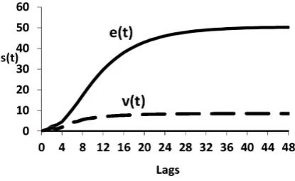
The solid impulse response labeled “e(t)” in Figure 7 is our estimate of their impulse response from their policy shock to their exchange rate. It shows that we can accurately replicate the h_{e s,}e

( )

L in their Figure 6. Both maximums are the

same, they peak at the same lag, converge to zero at the same lag and have a “notch” at the same lag. Neither impulse response function changes sign.

The solid response in Figure 8 labeled “e(t)” is the step response implied by the impulse response in Figure 7 labeled “e(t)”. It peaks after about 48 quarters. There is no sign of overshooting from their policy shock to their exchange rate. No transient step response exceeds the steady state response.

The dashed impulse response in Figure 7 is the impulse response from their policy variable itself to their exchange rate where the policy variable is exogen-ous as in [19]. The dashed line in Figure 8 is the corresponding step response. There is no evidence of overshooting from the policy variable to the exchange rate. No transient response of the exchange rate to a unit step in the policy vari-able in their PSVECM model is larger than the steady-state response.

[15] is the only article in Table 1 that provides the information necessary to test for Dornbusch overshooting or a delayed version of such overshooting ra-ther than for overshooting from a “Policy shock” to an exchange rate. Although it claims to find evidence of delayed overshooting, their preferred model rejects overshooting from both the policy shock and the policy variable itself to the ex-change rate.

6. Summary and Conclusions

[image:15.595.269.477.594.706.2]

Articles in Table 1 that claim to find Dornbusch overshooting or a delayed ver-sion of such overshooting base that claim on impulse response functions from

Figure 7. Impulse responses. -1

-0.50 0.51 1.52 2.53 3.54

0 4 8 12 16 20 24 28 32 36 40 44 48

s(t)

Lags

e(t)

[image:16.595.268.476.75.202.2]

DOI: 10.4236/tel.2019.95096 1504 Theoretical Economics Letters Figure 8. Step responses.

policy shocks to exchange rates that never have a significant change in sign and converge to zero. Our first and most important point is that, taking them as va-lid, such impulse response functions clearly reject overshooting from policy shocks to exchange rates. They imply corresponding step response functions where no transient response is greater than the steady state response. In other words, a permanent, rather than temporary, increase in what is called the “policy shock” would not cause the exchange rate to rise by more in the short run than in the long run.

Our second point is that the impulse responses in Table 1 neither support nor reject overshooting from policy variables themselves to exchange because they do not provide enough information. Only one article in Table 1 provides enough information to construct step responses from policy variables themselves to exchange rates. It rejects overshooting.

Put succinctly, the evidence in Table 1 rejects overshooting from policy shocks to exchange rates and provides no credible support for overshooting from policy variables themselves to exchange rates.

This article concentrates on the misinterpretation of impulse response func-tions in testing for Dornbusch and delayed overshooting; future research on Dornbusch and delayed overshooting needs to use a wider variety of econome-tric techniques and needs to evaluate impulse responses more carefully.

If this article is correct, then the articles in Table 1 that claim to find evidence of overshooting represent a shocking failure of peer review.

Acknowledgements

I want to thank Tom Doan at Estima, Chris Sims, an anonymous referee and particularly Michael Pippenger for their comments and suggestions. Any re-maining errors are of course mine.

Conflicts of Interest

The author declares no conflicts of interest regarding the publication of this paper.

References

DOI: 10.4236/tel.2019.95096 1505 Theoretical Economics Letters Shocks to Monetary Policy on Exchange Rates. The Quarterly Journal of Econom-ics, 110, 975-1009.https://doi.org/10.2307/2946646

[2] Levich, R.M. (1981) Overshooting in the Foreign Exchange Market. Occasional Pa-pers No. 5, Group of Thirty, New York.

[3] Grilli, V. and Roubini, R. (1996) Liquidity Models in Open Economies: Theory and Empirical Evidence. European Economic Review, 40, 847-859.

https://doi.org/10.1016/0014-2921(95)00096-8

[4] Cushman, D.O. and Zha, T. (1997) Identifying Monetary Policy in a Small Open Economy under Flexible Exchange Rates. The Journal of Monetary Economics, 39, 433-448.https://doi.org/10.1016/S0304-3932(97)00029-9

[5] Kim, S. and Roubini, N. (2000) Exchange Rate Anomalies in the Industrial Coun-tries: A Solution with a Structural VAR Approach. The Journal of Monetary Eco-nomics, 45, 561-586.https://doi.org/10.1016/S0304-3932(00)00010-6

[6] Kalyvitis, S. and Michaelides, A. (2001) New Evidence on the Effects of US Mone-tary Policy on Exchange Rates. Economic Letters, 71, 255-263.

https://doi.org/10.1016/S0165-1765(01)00375-5

[7] Faust, J. and Rogers, J.H. (2003) Monetary Policy’s Role in Exchange Rate Behavior.

Journal of Monetary Economics, 50, 1403-1424.

https://doi.org/10.1016/j.jmoneco.2003.08.003

[8] Kim, S. (2003) Monetary Policy, Foreign Exchange Intervention, and the Exchange Rate in a Unifying Framework. Journal of International Economics, 60, 355-386.

https://doi.org/10.1016/S0022-1996(02)00028-4

[9] Jang, K. and Ogaki, M. (2004) The Effects of Monetary Policy Shocks on Exchange Rates: A Structural Vector Error Correction Approach. Journal of the Japanese and International Economies, 18, 99-114.

https://doi.org/10.1016/S0889-1583(03)00042-X

[10] Kim, S. (2005) Monetary Policy, Foreign Exchange Policy, and Delayed Overshoot-ing. Journal of Money, Credit and Banking, 37, 775-782.

https://doi.org/10.1353/mcb.2005.0045

[11] Scholl, A. and Uhlig, H. (2008) New Evidence on the Puzzles: Results from Agnostic Identification on Monetary Policy and Exchange Rates. Journal of International Economics, 76, 1-13.https://doi.org/10.1016/j.jinteco.2008.02.005

[12] Bjørnland, H. (2009) Monetary Policy and Exchange Rate Overshooting, Dorn-busch Was Right after All. Journal of International Economics, 79, 64-77.

https://doi.org/10.1016/j.jinteco.2009.06.003

[13] Landry, A. (2009) Expectations and Exchange Rate Dynamics: A State-Dependent Pricing Approach. Journal of International Economics, 78, 60-71.

https://doi.org/10.1016/j.jinteco.2009.01.010

[14] Bouakez, H. and Normandin, M. (2010) Fluctuations in the Foreign Exchange Market: How Important Are Monetary Policy Shocks? Journal of International Economics, 81, 139-153.https://doi.org/10.1016/j.jinteco.2009.11.007

[15] Heinlein, R. and Krolzig, H.-M. (2012) Effects of Monetary Policy on the US Dol-lar/UK Pound Exchange Rate. Is There a “Delayed Overshooting Puzzle”? Review of International Economics, 20, 443-467.

https://doi.org/10.1111/j.1467-9396.2012.01033.x

DOI: 10.4236/tel.2019.95096 1506 Theoretical Economics Letters

https://doi.org/10.1007/s11079-016-9403-2

[17] Kim, S.-H., Moon, S. and Velasco, C. (2017) Delayed Overshooting: Is It an 80s Puzzle? Journal of Political Economy, 125, 1570-1598.

https://doi.org/10.1086/693372

[18] Kim, S. and Lim, L. (2018) Effects of Monetary Policy Shocks on Exchange Rate in Small Open Economies. Journal of Macroeconomics, 56, 324-339.

https://doi.org/10.1016/j.jmacro.2018.04.008

[19] Dornbusch, R. (1976) Expectations and Exchange Rate Dynamics. Journal of Politi-cal Economy, 84, 1161-1176.https://doi.org/10.1086/260506

[20] Leamer, E. (1983) Let’s Take the Con Out of Econometrics. The American Eco-nomic Review,73, 31-43.

[21] Enders, W. (2010) Applied Econometric Time Series. Wiley, Hoboken.

[22] Mittnick, S. and Zadrozny, P.A. (1993) Asymptotic Distributions of Impulse Res-ponses, Step Responses and Variance Decompositions of Estimated Linear Dynamic Models. Econometrica,61, 857-870.https://doi.org/10.2307/2951765