Structual Change Point Detection for Evolutional Networks

(1)

Structual Change Point Detection for Evolutional

Networks

Sadamori Koujaku, Mineichi Kudo, Ichigaku Takigawa, Hideyuki Imai

Abstract—We propose a change point detection algorithm for a sequence of graphs. Our algorithm focuses on the change of the structure of densely connected subgraphs (community structure) rather than the change of the link weights. In contrast to the traditional approaches, the algorithm can identify the structure change more sensitively. Experiments with a synthetic data and a real-world data of graphs showed that our algorithm can accurately locate the changed subgraph compared with some of the state-of-the-art algorithms

Index Terms—Anomaly detection, Evolution network, Mar-tingale, Spectral clustering

I. INTRODUCTION

G

RAPHS naturally arise in the current circumstance as seen in computer networks, World Wide Web, climate networks, social networks and biological networks. Accordingly anomaly detection of graphs has been gathering a great deal of attentions. For example, in the network intrusion detection, we want to find malicious messages (e.g spammers, port scanners) among many ordinary messages, and in the climate networks, we want to find anomalous phenomena (e.g heavy rain, storm) from signals obtained by several sensors.

Typical networks have dynamic nature and often keep growing or shrinking with time. Such dynamics should be taken into consideration for the design of anomaly detec-tors. In human/social networks represented by graphs with weighted undirected/directed links, a community that is a subgraph whose members are connected strongly to each other is a key factor to specify the characteristics of the graphs. In the view point of community, we can divide anomaly into that in the community structure and that in the community strength/activity.

A graph may change its communities in the member and/or in the way of connections, while another graph may strengthen or the connections among community members may be weaken. One example of the latter case is a lo-cal computer network where many messages have been exchanged regularly. In this example, a server and clients may make a community. Once a client is hacked, it may behave differently and send irregular messages to specific computers. Such anomaly would be detected as the change of link strength. Another example is a scientific network, where a node represents a scientist and a link represents the co-author relationship among scientists. A community in this network is seen as a group of scientists sharing similar

Manuscript received March 16, 2013; revised March 30, 2013. S. Koujaku is with the Graduate School of Information Science of Technology, Hokkaido University, Japan. M. Kudo, I.Takigawa and H.Imai are with Hokkaido University.

emails: (S.Koujaku, [email protected]). (M.Kodo,

[email protected]). (I.Takigawa, [email protected]). (H.Imai, [email protected]).

interests. The community may grow due to some boom of a specific subject and shrink due to maturity of the field. Such changes could be observed both in the community activity and community structure.

In this paper, we proposed an anomaly detector which has following key properties.

• It concentrates on communities

• It detects mainly the change of community structure. • It can work online.

We put the following assumptions on the input data: (1) no domain knowledge is available on the nature of network. (2) data arrives sequentially, (3) all links are not directed, (4) there exist some communities, that is subsets of dense connections.

The rest of papers are organized as follows. We briefly review some related works, in Section II. In Section III, our terminology and assumptions are presented. In Section IV, we describe the details of the proposed method. The experi-mental results are presented in Section V. We discussed the characteristics of our algorithm in section VI and summarized this paper in Section VII.

II. RELATEDWORK

In a static network, one goal is to find anomalous nodes or links which can be regarded as topological outliers. There have been proposed dozens of rarity/affinity measures for such outliers such as Random Work Similarity [1], [2], Information theoretic measure [3]–[5], density measure [6] and so on. We also use an affinity measure, but it finds transitions in the dynamics of graph rather than topologically rare nodes or links.

(2)

(a) Graph (b) Adjacency Matrix

2.0

2.0 2.0 0.5

1.5

[image:2.595.73.266.192.269.2]

1.5 1.5

Fig. 1. Illustration graph and its adjacency matrix

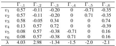
TABLE I

EIGENVECTORS ANDEIGENVALUES OF MATRIXXREPRESENTING A

GRAPH DEPICTED INFIG1

Γ_·,1 Γ·,2 Γ·,3 Γ·,4 Γ·,5 Γ·,6

v1 0.57 -0.11 -0.20 0 -0.71 -0.35

v2 0.57 -0.11 -0.20 0 0.71 -0.35

v3 0.58 -0.05 0.34 0 0 0.74

v4 0.13 0.57 0.72 0 0 -0.39

v5 0.08 0.57 -0.38 -0.71 0 0.16

v6 0.08 0.57 -0.38 0.71 0 0.16

λ 4.03 2.98 -1.34 -1.5 -2.0 -2.1

III. PREPARATION

A. Notation

Bold letters always denote random matrices. Superscript in parentheses denote time and subscripts i, j denote a row and a column of a matrix.

A graphGconsists of a setV of nodes and a setEof links. Furthermore, each link has a weightw∈[0,∞]representing the strength of connection. The matrix operator diag(·)and off-diag(·) decompose a matrix into the diagonal part and non diagonal part respectively.

A symmetric matrix X can be decomposed into X = ΓΛΓ0, whereΓis an orthonormal matrix with eigenvectors of

X in columns andΛis a diagonal matrix with corresponding real value eigenvalues. The column vectors of Γ are sorted in the descending order of its corresponding eigenvalues.

B. Community

Communities can be analyzed by the spectrum of a matrix representing a graph [12], [13]. To make clear the meaning of spectrum, let us consider an adjacency matrix X shown in Fig 1. Let us decompose X into X = ΓΛΓ0 where Γ is a matrix whose column is an eigenvector of X and Λ is a diagonal matrix whose diagonal elements are the real value eigenvalues. All of eigenvectors ofΓand the diagonal elements ofΛare shown in Table I. Here it is noted thatΓ_·1

andΓ_·2 correspond two communities C1={v1, v2, v3}and

C2 = {v4, v5, v6}, respectively. The eigenvalues represent

the strength of connectivity in the communities. The com-munity C1 has the strongest connectivity and C2 follows.

For a graph consists of l dense subgraphs, Peron Frobenius Theorem [14] guarantees that there exist l

positive eigenvalues expressing the strength of connectivity corresponding to the l communities and its corresponding eigenvector has large elements in its participating nodes. Such community is known as eigencluster [13] and the property of a graph can be separated into community structure and community activity.

DEFINITION (Community structure and activity) For a graph G expressed by an adjacency matrix X

with its eigen decomposition X = ΓΛΓ0, we call the positive eigenvalues of Λ the “community activity” and its corresponding eigenvector ofΓ the “community structure”.

When the number l of communities is known, we can find the largestl eigenvalues and eigenvectors asX 'ΓlΛlΓ0_l.

IV. PROPOSEDMETHOD

In this section, we present our algorithm to detect the changes in community structuresΓ. Our basic assumption is that the community structure is almost invariant over time, in other wards, dense/sparse connections would be unchanged even though their weights of links may change to some extent. In the following, we formalize the model of graph evolutions and introduce our algorithm.

A. Model

Let us consider a sequence of random graphs G =

n

G(1),G(2)_{, . . . ,}_G(t)o _{represented by adjacency matrices}

X = X(1)_,_X(2)_{, . . . ,}_X(T) _, _X _∈ _Rn×n_{, t} _{= 1}_,₂_,₃_..._. We assume that, as a normal state, the X(t) _{is generated}

independently from the following model:

X(t)= Γ(Λ +N(t))Γ0, t= 1,2, ..., (1) where the structure Γ is assumed not to change as well as activity Λ, while N(t) _{can change as a random} _noise _(not

always diagonal) matrix with mean zero matrix. The expectation of matrixX(t) _{is given by}

EX(t)= ΓΛΓ0+ Γ(EN(t))Γ0= ΓΛΓ0

Therefore, assuming ergodicity of X(t) for a period t ∈

[1, T], we estimate EX(t) as a sample mean as ¯

X= 1

T

X

t=1

X(t)'Γ (Λ) Γ0. (2) Then, we estimate Γ and Λ by decomposition of X¯. By choosing the principlelcomponents ofΓandΛ, we construct Γl andΛl as well. When the graph seems to be generated from this model, we regards the graph is in normal state, but if it does not, we consider the data is in abnormal state. In the follwoing, we quantify the deviation of the graph from this model and descriminate the normal and anomaly deviations.

B. Anomality Measure

Suppose that the model(Γ,Λ) changes to (˜Γ,Λ)˜ at time

t0. By monitoring the amount of fluctuation of corresponding

community structure Γ, this change is detected. In the following, we assume that Γ and Λ are already estimated from the past sequence by Eq. (2). We decomposeX(t) _by

multiplyingΓandΓ0 in both sides as

X(t)= ΓY(t)Γ0. (3)

At this time,Y(t) _{is not diagonal in general. Therefore, we}

separate the components into the diagonal part and the non-diagonal part as

X(t) = ΓY(t)Γ0

(3)

Similarly, we separate the Eq. (1) as

X(t) = Γ(Λ +N(t))Γ0

= Γ(Λ +diagN(t))Γ0+ Γ(off-diagN(t))Γ0. (5) Comparing Eq. (4) and Eq. (5), we can see that diag(Y(t)−

Λ) shows the regular fluctuation within communities, by noise N(t) and off-diagY(t) shows the fluctuation between communities. Both amounts are supposed to be small if the model does not change. However, if the structure changes fromΓto˜Γ, the amount of fluctuation caused by the change would be put on the second term of Eq. (4). Indeed, if the model is unchanged, that is, if Eq. (4) and Eq (5) are equal,

Eoff-diagY(t)

=E

off-diagN(t)

=O. (6)

Therefore we consider off-diagY(t)_{as the fluctuation in the}

community structure. Let us denote an anomaly score of the graph at timet as a(t), which is defined as

a(t) = ||off-diagY(t)||F = Tr

off-diagY(t)

0

off-diagY(t)

. (7)

where|| · ||F is the frobenius norm. The anomaly scorea(t) measures the amount of fluctuation in community structure and a high score implies that the model might be changed.

C. Martingale Test

From the sequence of anomaly scoresa(t),t= 1,2..., we would like to find the time when the community structure is changed. Because N(t)_, _t_{= 1}_,₂_... _{are generated from a}

stationary distribution, Y(t) _and _a(t)_, _t _{= 1}_,₂_{, ...} _{are also}

expected to have stationary properly as well. In other words, if the distribution ofa(t) _{has changed, we may consider the}

model changed.

To evaluate the changes in the distribution ofa(t)_{, we}

em-ploy a non-parameteric statistical test based onRandomized Power Martingale(RPM) [15]. Given a sequence of anomaly scores a(1)_{, a}(2)_{, ..., a}(t)_{, the RPM is defined as}

M(t)= t

Y

k=1

pˆ_k−1, (8)

where∈(0,1)and thepˆk is given by the pˆ-value function

ˆ

pk=

Pk i 1{a

(i)_{> a}(k)_}₊Pk

i ui1{a(i)=a(k)}

k (9)

where 1{S} becomes 1 in case that S is true otherwise 0 and ui is a random variable drawn from a uniform distribution over [0,1]. Here it is easily confirmed that the ˆ

p value are distributed uniformly over [0,1]. Therefore the conditional expectation of M(t) with respect to the past pˆ -valuespˆ1,pˆ2, ...,pˆtis given by

EhM(t)|pˆ1,pˆ2, ...pˆt

i

=M(t−1) Z 1

0

pˆt−1d =M(t−1). (10) This property “the expectation of the next value is the same as the current value” is called martingale and it satisfies Doob’s Maximal Inequality [16], [17]:

P

sup

0_≤k_≤t

M(k)≥1/δ

≤δ, (11)

Algorithm 1Pseudo code of proposed algorithm Input

A significance levelδ

Number of community structuresl

Number of first training dataτ0

Procedure

Set starting time of the sequenceτs=τ0+ 1

Initialize Martingale valueM(1) _{= 1}

whileNew dataX(t) _arrives_do

ift < τsthen

//Initial training

UpdateX¯ andΓby Eq. (2) else

//Detecting changes in the model

DecomposeX¯ into ΓandΛ.

Compute anomaly scorea(t) by Eq. (7) Compute p-valuep(t) by Eq. (9)

Update Radomized Power MartingaleM(t)by Eq. (8) ifM(t)≥1/δ then

Declare a change pointt

ResetM(t)_{= 1} _and_τ

s=t+τ0+ 1.

else

UpdateX¯ andΓby Eq. (2) end if

end if end while

TABLE II

OVERVIEWS OF ALGORITHMS

Algorithm Evaluated Variable Detectable Change

Proposed leigenvectors Intra-community links

EigenSpace [9] 1st eigenvector Densely connected nodes

EigenCompress [11] Eigenvalues Connectivity strength

whereδ∈(0,1]is a significance level. From this inequality, we see that a change happens with probability1−δ when

M(t) _exceeds ₁_/δ_{. The parameter} _{takes responsible for}

determining the sensitivity for the changes. Specifically, the smallincreases sensitiviness for the changes, but it causes false alarms. According to [15], it is appropriate to set in [0.9,1).

V. EXPERIMENT

We have conducted two experiments using one synthetic dataset and one real-world data. We compared the pro-posed method with other spectral approaches: EigenSpase [9], EigenCompress [11]. In EigenSpace, the most strongly connected subgraph is assumed to be invariant over time. EigenCpmpres, on the other hands, focuses on the activity of communities, thus detect the change of eigenvalues. These characteristics are summarized in Table II.

A. Synthetic data

In this experiment, we aimed to confirm that the changes of community structures are correctly detected by our algo-rithm. The basic structure of the graphs used in this experi-ment is shown in Fig 2. This basic graph consists of two com-munities CA = {v1, v2, v3, v4} and CB = {v5, v6, v7, v8}.

(4)

4 1

2

3 5

8 6

7

Fig. 2. Basic structure of the graph

4 1

2

3 5

8 6

7

4 1

2

3 5

8 6

7

Scenario 1 Scenario 2

Scenario 4 Scenario 3

4 1

2

3 5

8 6

7

Strengthened

4 1

2

3 5

8 6

7

Strengthened _Weakened

Strengthened

Fig. 3. Different 4 scenarios of changing.

The width of alink shows the strength of connections

TABLE III

FOUR DIFFERENTSCENARIOS OF CHANGING

Scenario of changing (µAA, µBB, µAB)

0 Before change (0.8,0.6,0.2)

1 Links inCAare strengthened (1.0,0.6,0.2)

2 Links inCB are weaken (0.8,0.4,0.2)

3 The connectivity ofCB is maximized (0.8,1.0,0.2)

4 Links between communities are strengthened (0.8,0.6,0.4)

weight of linkwi,j between nodesvi andvj as

wi,j=

  

µAA+ 0.2u (vi, vj∈CA)

µBB+ 0.2u (vi, vj ∈CB)

µAB+ 0.2u (vi∈CA, vj∈CB)

, (12)

where µAA, µBB and µAB are basic weights of whithin

communities and between communities. A sequence consists of 200 graphs was generated according to this model. We tested 4 scenarios as shown in Fig (3), in which a change occures at time t0 = 100and the parameters were changed

to(µ0_AA, µ0_BB, µ0_AB)as shown in Table III. The scenarios 1, 2 and 3 change the weights of intra-communities and the scenario 4 changes in the weights of inter-communities. We constructed a dataset consists of 100 seqeunces generated by unchanged model (12) and 100 sequences including a change according to one of above senarios and tested whether the algorithm distinguishes changed cases and unchanged cases correctly or not.

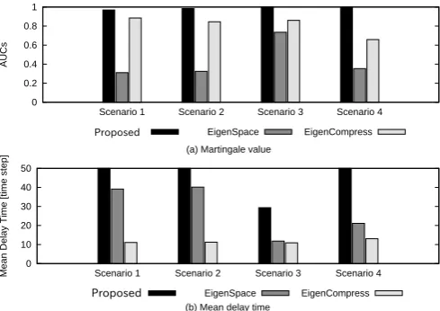
We measured the area under curve (AUC) of the graph as the plane of which horizontal axis is the false alarm rate and vertical axis is recall value (Fig. 4). The AUC was calculated by the trapezoid integration. While we gradually changed the value of parameters of the algorithms, we measured the false alarm rate and recall. For the EigenSpace and the proposed method, the significance level δwas changed. For EigenCompress, the threshold value for the anomaly scores was changed since this method does not have any parameter to determine the significance level.

The other parameters were set so as to achieve the highest average AUCs over the 4 scenarios. For EigenSpace, the learning parameter β = 0.03and the window size w= 30. The number of eigenvalues monitored by EigenCompress was 3. For our algorithm, we setl= 2 and= 0.95.

The AUCs are summarized in Fig 5 (a). As expected from their characteristics, Eigenspace succeeded in detecting only the change of the structure of the most densely connected community, that is, the change of scenario 3 (the strongest community moves from CA toCB), while EigenCompress succeeded in detecting the change of activities of both communities in scenarios 1, 2 and 3. The reason why the proposed algorithm aiming the detection of the changes of

0 0.2 0.4 0.6 0.8 1

Recall

False alarm rate

(a) Proposed

EigenSpace EigenCompress

0 0.2 0.4 0.6 0.8 1

Recall

False alarm rate

(b) Proposed

0 0.2 0.4 0.6 0.8 1

Recall

False alarm rate

(c) Proposed

0 0.2 0.4 0.6 0.8 1

Recall

False alarm rate

(d) Proposed

[image:4.595.304.549.264.437.2]

Fig. 4. ROC curves in four scenarios: (a) Scenario 1. (b) Scenario 2, (c)

Scenario 3 and (d) Scenario 4

0 0.2 0.4 0.6 0.8 1

Scenario 1 Scenario 2 Scenario 3 Scenario 4

A

U

C

s

(a) Martingale value

Proposed EigenSpace EigenCompress

0 10 20 30 40 50

Scenario 1 Scenario 2 Scenario 3 Scenario 4

Me

a

n

D

e

la

y

T

ime

[t

ime

st

e

p

]

(b) Mean delay time

Proposed EigenSpace EigenCompress

Fig. 5. Comparison of (a).AUCs of false alarm rate vs. recall and (b).mean delay time in 4 scenarios

the community structure succeeded in detection of the inter-community changes is that the activity change also derives the structure change. For example, in scenario 1, the right community relatively vanished after strengthening of the left community.

Next, we examined the mean delay time (MDT) of these algorithms. To unify the sensitivity of detectors, we set the value of parameters of algorithms as follows. For EigenSpace and the proposed method, we set the significance level to 0.05. For EigenCompress, the threshold values is determined such that the ratio of anomaly scores over the threshold is 0.05.

Fig 5 (b) shows the result of MDT. We observe that the proposed algorithm has the longest delay in all scenarios. This is because the the martingaleM(t) _{exceeds the}

bound-ary (11) after observing several high anomay scores, while other methods issues alarm onece one high anomaly score is observed.

B. Enron email dataset

(5)

TABLE IV

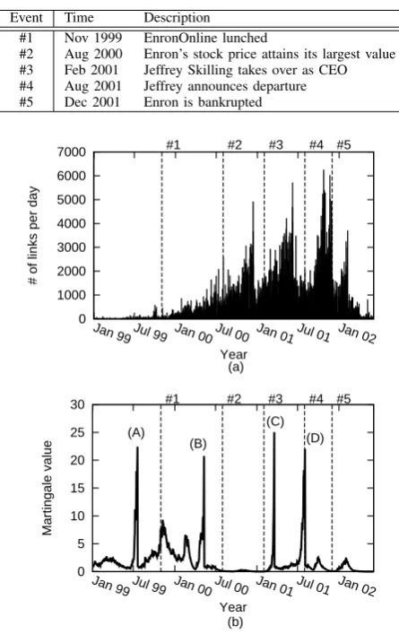
EVENTS INENRONINC FROMJANUARY1999TOJURY2002

Event Time Description

#1 Nov 1999 EnronOnline lunched

#2 Aug 2000 Enron’s stock price attains its largest value

#3 Feb 2001 Jeffrey Skilling takes over as CEO

#4 Aug 2001 Jeffrey announces departure

#5 Dec 2001 Enron is bankrupted

0 5 10 15 20 25 30

Jan₉₉_{Jul 99 Jan 00 Jul 00 Jan 01}_{Jul 01 Jan 02}

Mart

in

ga

le

va

lu

e

Year

#1 #2 #3 #4 #5

(A)

(B)

(C) (D)

(b) 0

1000 2000 3000 4000 5000 6000 7000

Jan

99Jul99 Jan₀₀Jul00 Jan₀₁Jul 01 Jan 02

#

of

links

pe

r

d

ay

Year

#1 #2 #3 #4 #5

[image:5.595.56.279.74.428.2]

(a)

Fig. 6. (a) # of Emails exchanged in a day. (b) Martingale values

the number of emails exchanged between the corresponding two employees. In this graph, the most densely connected subgraph corresponds to an executive committee exchanging many emails to run the company. The other subgraphs consist of communications between executives and employees in corresponding sections.

The special events happened during this period are sum-marized in Table IV and the number of emails in each day is shown in Fig 6 (a). We see that the number of emails started increasing after the event #1 according to the company growth. Before the event #5, it reached its peak since the executives exchanged many emails to prepare the risk of possible bankrupt.

We examined whether our algorithm detects changes re-lated to these events. We observed that there were more than 3 positive eigenvalues over this period, and thus we setl= 3. It might be hard to locate the cause of changes after a long delay and therefore we setδ= 0.05and= 0.9 in order to detect the changes quickly.

The martingale values were plotted in Fig 6 (b). The four of changing time points were detected : (A) 06 Jul 1999, (B) 07 Mar 2000, (C) 13 Jan 2001 and (D) 30 May 2001. Only #4 event is detected as a change. To interpret the result, we have to consider again what kind of changes are detected by the proposed method. As seen in Fig 6 (b), our change detector waits until certain amount of evidence of strangeness

(a) untill (A) (b) Period (A) - (B)

(c) Period (B) - (C) (d) Period (C) - (D)

Vice President Director

Employee Employee

Employee

Employee Vice President Employee

Employee CEO

Employee Employee

Vice President Vice President

Vice President

Employee Employee

Employee

Employee CEO

Employee Employee

Vice President

Employee Employee

Employee

Employee CEO

Employee Employee

Vice PresidentVice President

Vice President

Employee Employee

Employee

Employee CEO

Employee Employee

Vice President

Fig. 7. Illustration of the time series of the subgraphs. The width of a link shows the amount of emails exchanged.

is gathered, so that it does not detect an abrupt change but a gradual change to some extent. In this sense, our detector might have detected changing points of organizational life cycle: birth, growth, maturity, decline and death. Under this explanations, the period before (A) corresponds to “birth” , the period (A)-(B) to “growth”, the period (B)-(C) to “maturity”, the period (C)-(D) “decline” and the period (D)-to “death”. These interpretation may be supported by the events #1-#5 happened in the corresponding period, e.g the highest stock price was marked (#2) just after the end of growth period.

To examine the validity of those interpretations, we visual-ized the graphs corresponding to these periods. Fig 7 shows the time series of subgraphs consists of the nodes corre-sponding to 3 strongest communities. Although it might be a little intentional, Fig 7 (a) -Fig 7 (d) look as showing (a) the CEO intensively listens to the opinion of external members and two sections worked for lunching “EnronOnline”, (b) 4 sections are organized, (c) new employees participated and also some employees moved their sections, and (d) intensive discussion is made among vice presidents.

(6)

VI. DISCUSSION

A. Detectable changes

The proposed algorithm detects not only the change of community structure, but also the change of community activity. This is reasonable in some sense. Strictly speaking, the community structure and community activity cannot be separated so clearly because the structure may change due to the heavily weakened links or strengthened links.

Our algorithm is slow to report a change compared to the other methods. The competitors are designed to detect the abrupt changes as it happens, but our algorithm detects changes after gathering a necessary amount of evidence. Therefore, it takes longer delay and thus the temporal change might be missed. It may be possible to use our algorithm to report a past change later, which might be useful in some applications.

B. Computational Complexity

The eigen decomposition of X¯ costs O(ln2) and the multiplication of Γto compute off-diagY costsO(n2). The anomaly score is computed at cost ofO(n2)and therefore the total cost of computing anomly score isO(ln2+n2+n2) = O(ln2). If we employ a heap-sort algorithm for ordering anomaly scores,pˆvalue in Eq. (9) can be computed at cost of O(TlogT)whereT is the number of data in a segment. Since n is very large in general compared to T, the total computation cost becomes O(ln2 ₊_T_log_T₎ _{' O}₍_ln2₎_.

However, it can be efficiently reduced toO(l3₎_{by employing}

the incremental spectrum updating techniques [19], [20] for the eigen decomposition ofX¯.

C. Laplacian Matrix and Modularity Matrix

In this paper, we focused on the changes of the communi-ties on the basis of the eigenvectors of an adjacency matrix. In this case, the community is a group of nodes with dense connections. Such a property “an eigenvector of a matrix expresses affinities among nodes” can be also dealt with the

Laplacian Matrix[12], [21] and theModularity Matrix[22], [23]. In the future, we will compare these with the proposed method.

VII. CONCLUSION

In this paper, we have proposed an anomaly detection algorithm for evolutional networks. We have assumed that a community is a dense subgraph and the invariant of the structure of a community can be confirmed by the unchanged eigenvectors. The traditional approaches monitor mainly the strongest community, while our approach monitors many principle communities. This algorithm also outperforms the others in detection of a change of activity between different communities.

We compared our algorithm with two state-of-the-art algo-rithms and confirmed its effectiveness. On the other hands, its response was three times later than the other methods. The results on the email communication showed that our algorithm detected changes longer or shorter before the critical event happens.

Further analysis is needed to reduce the delay and the property of other matrix would be more cleared by compar-ison with our algorithm.

REFERENCES

[1] D. Chakrabarti and C. Faloutsos, “Neighborhood Formation and

Anomaly Detection in Bipartite Graphs,” inFifth IEEE International

Conference on Data Mining (ICDM’05). IEEE, 2005, pp. 418–425. [2] H. D. K. Moonesinghe and P.-N. Tan, “OutRank: A GRAPH-BASED OUTLIER DETECTION FRAMEWORK USING RANDOM WALK,”International Journal on Artificial Intelligence Tools, vol. 17, no. 01, pp. 19–36, Feb. 2008.

[3] D. Chakrabarti, “AutoPart: Parameter-Free Graph Partitioning and

Out-lier Detection,” inKnowledge Discovery in Databases: PKDD 2004,

ser. Lecture Notes in Computer Science, J.-F. Boulicaut, F. Esposito,

F. Giannotti, and D. Pedreschi, Eds. Springer Berlin / Heidelberg,

2004, vol. 3202, pp. 112–124.

[4] W. Eberle and L. Holder, “Anomaly detection in data represented as graphs,”Intelligent Data Analysis, vol. 11, no. 6, pp. 663–689, 2007. [5] C. C. Noble and D. J. Cook, “Graph-based anomaly detection,” in

Proceedings of the ninth ACM SIGKDD international conference on Knowledge discovery and data mining, ser. KDD ’03, vol. 1, ACM. New York, NY, USA: ACM, 2003, pp. 631–636.

[6] V. Hautamaki, I. Karkkainen, and P. Franti, “Outlier detection using

k-nearest neighbour graph,” inProceedings of the 17th International

Conference on Pattern Recognition, 2004. ICPR 2004. IEEE, 2004, pp. 430–433 Vol.3.

[7] J. Sun, C. Faloutsos, S. Papadimitriou, and P. S. Yu, “GraphScope,” inProceedings of the 13th ACM SIGKDD international conference on Knowledge discovery and data mining - KDD ’07. New York, New York, USA: ACM Press, 2007, p. 687.

[8] S. Papadimitriou, J. Sun, and P. Yu, “Local Correlation Tracking

in Time Series,” in Sixth International Conference on Data Mining

(ICDM’06). IEEE, Dec. 2006, pp. 456–465.

[9] T. Ide and H. Kashima, “Eigenspace-based anomaly detection in

computer systems,” inProceedings of the 2004 ACM SIGKDD

inter-national conference on Knowledge discovery and data mining - KDD

’04, ser. KDD ’04. New York, New York, USA: ACM Press, 2004,

p. 440.

[10] T. Id´e and K. Inoue, “Knowledge discovery from heterogeneous

dynamic systems using change-point correlations,”Proc. SIAM Intl.

Conf. Data Mining, no. Sdm 05, pp. 571–575, 2005.

[11] S. Hirose, K. Yamanishi, T. Nakata, and R. Fujimaki, “Network

anomaly detection based on Eigen equation compression,” in

Proceed-ings of the 15th ACM SIGKDD international conference on Knowledge discovery and data mining - KDD ’09. New York, New York, USA: ACM Press, 2009, p. 1185.

[12] L. Hagen and A. Kahng, “New spectral methods for ratio cut

partition-ing and clusterpartition-ing,”IEEE Transactions on Computer-Aided Design of

Integrated Circuits and Systems, vol. 11, no. 9, pp. 1074–1085, 1992. [13] S. Sarkar and K. Boyer, “Quantitative measures of change based

on feature organization: eigenvalues and eigenvectors,”Proceedings

CVPR IEEE Computer Society Conference on Computer Vision and Pattern Recognition, pp. 478–483, 1996.

[14] A. Berman and R. J. Plemmons,Nonnegative matrices in the

math-ematical sciences, ser. Computer science and applied mathematics. Academic Press, 1979.

[15] V. Vovk, I. Nouretdinov, and A. Gammerman, “Testing exchangeability

on-line,” in MACHINE LEARNING-INTERNATIONAL WORKSHOP

THEN CONFERENCE-, vol. 20, no. 2, 2003, p. 768.

[16] J. L. Doob, “Boundary properties of functions with finite Dirichlet integrals,”Ann. Inst. Fourier, vol. 12, pp. 573–621, 1962.

[17] D. Williams,Probability With Martingales, ser. Cambridge

Mathemat-ical Textbooks. Cambridge University Press, 1991.

[18] [Online]. Available: http://www.cs.cmu.edu/ enron

[19] H. Zha and H. D. Simon, “On Updating Problems in Latent Semantic Indexing,”SIAM Journal on Scientific Computing, vol. 21, no. 2, pp. 782–791, Jan. 1999.

[20] C. Dhanjal, R. Gaudel, and S. Cl´emenc¸on, “Efficient Eigen-updating for Spectral Graph Clustering,” p. 25, Jan. 2013.

[21] J. Malik, “Normalized cuts and image segmentation,”IEEE

Transac-tions on Pattern Analysis and Machine Intelligence, vol. 22, no. 8, pp. 888–905, 2000.

[22] M. E. J. Newman, “Detecting community structure in networks,”The

European Physical Journal B - Condensed Matter, vol. 38, no. 2, pp. 321–330, Mar. 2004.

[23] M. Newman, “Modularity and community structure in networks.”